Formation of Terrestrial Planets from Protoplanets under a Realistic Accretion Condition

Abstract

The final stage of terrestrial planet formation is known as the giant impact stage where protoplanets collide with one another to form planets. So far this stage has been mainly investigated by $N$-body simulations with an assumption of perfect accretion in which all collisions lead to accretion. However, this assumption breaks for collisions with high velocity and/or a large impact parameter. We derive an accretion condition for protoplanet collisions in terms of impact velocity and angle and masses of colliding bodies, from the results of numerical collision experiments. For the first time, we adopt this realistic accretion condition in $N$-body simulations of terrestrial planet formation from protoplanets. We compare the results with those with perfect accretion and show how the accretion condition affects terrestrial planet formation. We find that in the realistic accretion model, about half of collisions do not lead to accretion. However, the final number, mass, orbital elements, and even growth timescale of planets are barely affected by the accretion condition. For the standard protoplanetary disk model, typically two Earth-sized planets form in the terrestrial planet region over about $10^{8}$ years in both realistic and perfect accretion models. We also find that for the realistic accretion model, the spin angular velocity is about 30% smaller than that for the perfect accretion model that is as large as the critical spin angular velocity for rotational instability. The spin angular velocity and obliquity obey Gaussian and isotropic distributions, respectively, independently of the accretion condition.

1 INTRODUCTION

It is generally accepted that the final stage of terrestrial planet formation is the giant impact stage where protoplanets or planetary embryos formed by oligarchic growth collide with one another to form planets (e.g., Wetherill, 1985; Kokubo & Ida, 1998). This stage has been mainly studied by $N$-body simulations. So far all $N$-body simulations have assumed perfect accretion in which all collisions lead to accretion (e.g., Agnor et al., 1999; Chambers, 2001). However, this assumption would be inappropriate for grazing impacts that may result in escape of an impactor or hit-and-run. By performing Smoothed-Particle Hydrodynamic (SPH) collision simulations, Agnor & Asphaug (2004) estimated that more than half of all collisions between like-sized protoplanets do not simply result in accumulation of a larger protoplanet, and this inefficiency lengthens the timescale of planet formation by a factor of 2 or more, relative to the perfect accretion case. The accretion inefficiency can also change planetary spin. Kokubo & Ida (2007) found that under the assumption of perfect accretion, the typical spin angular velocity of planets is as large as the critical spin angular velocity for rotational instability. However, in reality, the grazing collisions that have high angular momentum are likely to result in a hit-and-run, while nearly head-on collisions that have small angular momentum lead to accretion. In other words, small angular momentum collisions are selective in accretion. Thus, the accretion inefficiency may lead to slower planetary spin, compared with the perfect accretion case.

The goal of this paper is to clarify the statistical properties of terrestrial planets formed by giant impacts among protoplanets under a realistic accretion condition. We derive an accretion condition for protoplanet collisions in terms of collision parameters, masses of colliding protoplanets and impact velocity and angle, by performing collision experiments with an SPH method. We implement the realistic accretion condition in $N$-body simulations and probe its effect to further generalize the model of terrestrial planet formation. We derive the statistical dynamical properties of terrestrial planets from results of a number of $N$-body simulations and compare the results with those in Kokubo et al. (2006) and Kokubo & Ida (2007) where perfect accretion is adopted.

In section 2, we outline the initial conditions of protoplanets and the realistic accretion condition. Section 3 presents our results, where we show the statistics of collision parameters and basic dynamical properties of planets. Section 4 is devoted to a summary and discussions.

2 METHOD OF CALCULATION

2.1 Initial Conditions

We perform $N$-body simulations of terrestrial planet formation starting from protoplanets. We consider gas-free cases without giant planets residing outside the terrestrial planet region to clarify the basic dynamics. To compare with the results with perfect accretion, we adopt the same protoplanet system as those in Kokubo et al. (2006) and Kokubo & Ida (2007), which is formed by oligarchic growth from a planetesimal disk whose surface density distribution is given by

$$\Sigma=10\left(\frac{r}{\rm 1AU}\right)^{-3/2}{\rm gcm}^{-2},$$ (1)

with inner and outer edges, $r_{\rm in}=0.5$AU and $r_{\rm out}=1.5$AU, where $r$ is the radial distance from the central star. This disk model is the standard disk model for solar system formation and 50% more massive than the minimum-mass disk (Hayashi, 1981). In the oligarchic growth model, the mass of a protoplanet $M$ is given by the isolation mass

$$M_{\rm iso}\simeq 2\pi ab\Sigma=0.16\left(\frac{\tilde{b}}{10}\right)^{3/2}\left(\frac{a}{1{\rm AU}}\right)^{3/4}M_{\oplus},$$ (2)

where $a$ is the semimajor axis, $b$ is the orbital separation between adjacent protoplanets, $\tilde{b}=b/r_{\rm H}$, $r_{\rm H}$ is the Hill radius $r_{\rm H}=(2M_{\rm iso}/3M_{\odot})^{1/3}a$ of the protoplanet, $M_{\odot}$ is the mass of the central star, and $M_{\oplus}$ is Earth mass (Kokubo & Ida, 2000). We set the orbital separation of protoplanets as $\tilde{b}=10$ that is the typical value in $N$-body simulations (e.g., Kokubo & Ida, 2000, 2002). The initial eccentricities $e$ and inclinations $i$ of protoplanets are given by the Rayleigh distribution with dispersions $\langle e^{2}\rangle^{1/2}=2\langle i^{2}\rangle^{1/2}=0.01$ (the unit of $i$ is radian) (Ida & Makino, 1992). We set the bulk density of protoplanets as $\rho=3$ gcm^-3. The initial protoplanet system has the number of protoplanets $n=16$ in $r_{\rm in}\leq a\leq r_{\rm out}$, total mass $M_{\rm tot}\simeq 2.3M_{\oplus}$, specific angular momentum $j\simeq 0.95j_{\oplus}$, and mean semimajor axis $\bar{a}=j^{2}/GM_{\odot}=0.91$AU, where $j_{\oplus}=\sqrt{GM_{\odot}a_{\oplus}}$ and $a_{\oplus}$ is the semimajor axis of Earth. For each accretion model, we perform 50 runs with different initial angular distributions of protoplanets.

2.2 Orbital Integration

The orbits of protoplanets are calculated by numerically integrating the equations of motion of protoplanets. We set the mass of the central star equal to solar mass. For numerical integration, we use the modified Hermite scheme for planetary $N$-body simulation (Kokubo et al., 1998; Kokubo & Makino, 2004) with the hierarchical timestep (Makino, 1991). For the calculation of mutual gravity among protoplanets, we use the Phantom GRAPE scheme (Nitadori et al., 2006). The simulations follow the evolution of protoplanet systems for $3\times 10^{8}$ years until only a few planets remain.

2.3 Accretion Condition

During orbital integration, when two protoplanets contact, a collision occurs. We define an impactor/target as a smaller/larger one of two colliding bodies. We obtained a realistic accretion condition of protoplanets by performing SPH collision simulations. The standard SPH method (Monaghan, 1992; Canup, 2004) was used with the Tillotson equation of state (Melosh, 1989). We assumed differentiated protoplanets with 30% core and 70% mantle in mass. Protoplanets were represented by 20,000 particles in most runs and 60,000 particles in high-resolution runs. We systematically varied the mass ratio of the impactor and target as $M_{\rm imp}/M_{\rm tar}=1$, 2/3, 1/2, 1/3, 1/4, 1/6, and 1/9, their total mass as $M_{\rm col}=M_{\rm imp}+M_{\rm tar}=0.2$-$2M_{\oplus}$, and the impact velocity and angle as $v_{\rm imp}=1.0$-$3.0v_{\rm esc}$ at 0.02 or $0.2v_{\rm esc}$ intervals and $\theta=0^{\circ}$-$75^{\circ}$ at $15^{\circ}$ intervals, where $v_{\rm esc}$ is the mutual surface escape velocity $v_{\rm esc}=[2GM_{\rm col}/(R_{\rm imp}+R_{\rm tar})]^{1/2}$, $R_{\rm imp}$ and $R_{\rm tar}$ are the radii of the impactor and target, and $\theta$ is the angle between the surface normal and the impact trajectory ($\theta=0^{\circ}$ for a head-on collision and $\theta=90^{\circ}$ for a grazing encounter). Based on the results of SPH collision simulations, we derived an empirical formula for the critical impact velocity, below which a collision leads to accretion, in terms of the masses of the impactor and target and the impact angle as

$$\frac{v_{\rm cr}}{v_{\rm esc}}=c_{1}\left(\frac{M_{\rm tar}-M_{\rm imp}}{M_{\rm col}}\right)^{2}(1-\sin\theta)^{5/2}+c_{2}\left(\frac{M_{\rm tar}-M_{\rm imp}}{M_{\rm col}}\right)^{2}+c_{3}(1-\sin\theta)^{5/2}+c_{4},$$ (3)

where $c_{1}=2.43$, $c_{2}=-0.0408$, $c_{3}=1.86$, and $c_{4}=1.08$ are numerical constants. The critical impact velocity is a decrease function of $\sin\theta$ as seen in Figure 1. For collisions of equal-mass protoplanets, this condition agrees well with the results of SPH collision simulations by Agnor & Asphaug (2004). The reason for this agreement is that we performed almost the same collision simulations by essentially the same method, which confirms the robustness of the results. The details of the collision simulations and the accretion condition will be presented in a separate paper. In the realistic accretion model we use this accretion condition. In accretion, the position and velocity of the center of mass and the angular momentum are conserved.

If the impact velocity $v=|\mbox{\boldmath$v$}|=\sqrt{v_{\rm n}^{2}+v_{\rm t}^{2}}$ is higher than $v_{\rm cr}$, two colliding bodies are bounced with the rebound velocity $\mbox{\boldmath$v$}^{\prime}$, $v^{\prime}_{\rm n}=0$ and $v^{\prime}_{\rm t}=\max(v_{\rm t},v_{\rm esc})$, where subscripts n and t mean normal and tangential components of the velocity, respectively. The change in spin angular momentum brought about by hit-and-run collisions is not taken into account since it is usually much smaller than that caused by accretionary collisions. These prescriptions follow the results of the collision experiments.

We assume that, initially, protoplanets have no spin angular momenta. We track the spin angular momentum of planets resulting from accretion. When accretion occurs, the orbital angular momenta of two colliding bodies about their center of mass and their spin angular momenta are added to the spin angular momentum of a merged body. The spin angular velocity of planets is computed by assuming a sphere of uniform density, in other words, the moment of inertia $I=(2/5)MR^{2}$, where $M$ and $R$ are the planetary mass and radius, respectively.

3 RESULTS

We compare the results of the realistic accretion model to those of the perfect accretion model (Kokubo et al., 2006; Kokubo & Ida, 2007). The statistics of collision parameters and basic dynamical properties of planets derived from 50 runs for each accretion model are summarized in Tables 1 and 2.

3.1 Statistics of Collision Parameters

We record the collision parameters in all runs. The numbers of hit-and-run $n_{\rm har}$ and accretionary $n_{\rm acc}$ collisions are summarized in Table 1. In the realistic accretion model, the total number of collisions in 50 runs is 1211. In a run, the average numbers of hit-and-run and accretionary collisions are $\langle n_{\rm har}\rangle=11.8$ and $\langle n_{\rm acc}\rangle=12.4$, respectively, which means on average 49% of collisions results in hit-and-run. Note that the average number of accretionary collisions for the realistic accretion model is almost the same as that for the perfect accretion model. This suggests that the growth timescale of planets is independent of the accretion model. We will discuss this later.

On the giant impact stage, the last one or a few large collisions determine the final spin angular momentum of planets (Agnor et al., 1999; Kokubo & Ida, 2007). In this case, the spin angular velocity is estimated as

$$\omega\simeq\frac{5}{\sqrt{2}}\langle g(\gamma)^{2}\rangle^{1/2}\langle\sin\theta^{2}\rangle^{1/2}\langle\nu^{2}\rangle^{1/2}\omega_{\rm cr},$$ (4)

where $\gamma=M_{\rm imp}/M_{\rm col}$, $g(\gamma)=\gamma(1-\gamma)\left[\gamma^{1/3}+(1-\gamma)^{1/3}\right]^{1/2}$, and $\nu=v/v_{\rm esc}$. The critical spin angular velocity for rotational instability $\omega_{\rm cr}$ is given by

$$\omega_{\rm cr}=\left(\frac{GM}{R^{3}}\right)^{1/2}=3.3\left(\frac{\rho}{3{\rm gcm}^{-3}}\right)^{1/2}{\rm hr}^{-1},$$ (5)

where $\rho$ is the material density.

In Figure 1, we plot the scaled impact velocity $\nu$ against $\sin\theta$ for all collisions in all runs for the realistic accretion model. We show that only collisions with small $\nu$ and/or $\sin\theta$ can lead to accretion due to the realistic accretion condition. For collisions forming Earth-sized planets ($M>M_{\oplus}/2$), the RMS values of the collision parameters are $\langle g(\gamma)^{2}\rangle^{1/2}=0.24$, $\langle\sin^{2}\theta\rangle^{1/2}=0.62$, and $\langle\nu^{2}\rangle^{1/2}=1.19$ for the realistic accretion model, and $\langle g(\gamma)^{2}\rangle^{1/2}=0.25$, $\langle\sin^{2}\theta\rangle^{1/2}=0.71$, and $\langle\nu^{2}\rangle^{1/2}=1.40$ for the perfect accretion model. The RMS impact parameter $\langle\sin^{2}\theta\rangle^{1/2}$ for the realistic accretion model is smaller than that for the perfect accretion model since small impact parameters are selective in the realistic accretion model. Also, for the same reason, the RMS impact velocity $\nu$ for the realistic accretion model is slightly smaller than that for the perfect accretion model. Using these RMS values, we obtain the typical spin angular velocity resulting from an accretionary collision as 2.0 hr^-1 and 2.8 hr^-1 for the realistic and perfect accretion models, respectively.

3.2 Statistics of Basic Dynamical Properties

The average values with standard deviations for basic dynamical properties of planets: the number of planets, $n$, the number of Earth-sized planets with $M>M_{\oplus}/2$, $n_{M}$, the number of planets in $r_{\rm in}\leq a\leq r_{\rm out}$, $n_{a}$, the in-situ accretion efficiency $f_{a}=M_{a}/M_{\rm tot}$ where $M_{a}$ is the total mass of planets in $r_{\rm in}\leq a\leq r_{\rm out}$, and the growth timescale $T_{\rm grow}$ defined as duration of accretion for each planet that undergoes at least two accretionary collisions are summarized in Table 1. The mass and orbital elements (semimajor axis $a$, eccentricity $e$, and inclination $i$) of the largest and second-largest planets are summarized in Table 1.

First, we find no substantial differences between the results of the two accretion models. In both models, a typical resultant system consists of two Earth-sized planets and one or two smaller planets that are as large as the initial protoplanets (Kokubo et al., 2006). The two Earth-sized planets tend to form inside the initial distribution of protoplanets. The resultant system for the realistic accretion model tends to be slightly wider than that for the perfect accretion model, which can be seen as having slightly larger $\langle n\rangle$ and smaller $\langle n_{a}\rangle$ and $\langle f_{a}\rangle$. This is because the realistic accretion model experiences more close encounters between protoplanets that diffuse the system. It should be noted that though about half of collisions do not lead to accretion, this accretion inefficiency does not lengthen the growth timescale by a factor of two or more, relative to the perfect accretion model as expected by Agnor & Asphaug (2004). The growth timescale for the realistic accretion model is only slightly longer than that for the perfect accretion model. This is because even though collisions do not lead to accretion, the colliding bodies stay on the colliding orbits after the collision and thus the system is unstable and the next collision takes place shortly. In fact, the mean accretionary collision time for the realistic accretion model is $T_{\rm col}=11.1\pm 29.3\times 10^{6}$ years, which is as long as the mean collision time for the perfect accretion model $T_{\rm col}=10.3\pm 30.3\times 10^{6}$ years. On the other hand, in the realistic accretion model, the mean collision time after a hit-and-run collision is short as $T_{\rm col}=3.6\pm 9.1\times 10^{6}$ years, where 38% of collisions is for the same pair and its mean collision time is even shorter as $T_{\rm col}=2.1\pm 5.6\times 10^{6}$ years.

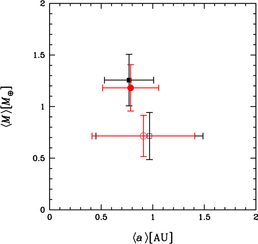
Figure 2: Average semimajor axes and masses of the largest (filled symbols) and second-largest (open symbols) planets for realistic (circle) and perfect (square) accretion models. The error bars indicate 1-$\sigma$.

Figure 2 shows the average masses of the largest and second-largest planets against their average semimajor axes. We find that there are no differences in either mass or semimajor axis of the planets for the realistic and perfect accretion models. The largest planets with $M\simeq 1.2M_{\oplus}$ tend to form around $\langle a_{1}\rangle\simeq 0.8$ AU, while the second-largest planets with $M\simeq 0.7M_{\oplus}$ is widely scattered in the initial protoplanet region. We also find no difference in their eccentricities and inclinations, and those are $\simeq 0.1$. These eccentricities and inclinations are an order of magnitude larger than the proper eccentricities and inclinations of the present terrestrial planets. Some damping mechanism such as gravitational drag (dynamical friction) from a dissipating gas disk (Kominami & Ida, 2002) or a residual planetesimal disk (Agnor et al., 1999) is necessary after the giant impact stage.

3.3 Statistics of Spin

In 50 runs of the realistic and perfect accretion models, we have 128 and 124 planets that experience at least one accretionary collision, respectively. The average values of each component of the spin angular velocity $\omega$ of the planets and its dispersion $\sigma$ are summarized in Table 2 together with the Root-Mean-Square (RMS) spin angular velocity $\langle\omega^{2}\rangle^{1/2}$ and the spin anisotropy parameter $\beta=\langle\omega_{z}^{2}\rangle/\langle\omega^{2}\rangle$.

The spin angular velocity averaged in mass bins against mass is shown in Figure 3a. We show clearly that the average angular velocity is almost independent of mass for both accretion models. For the perfect accretion model, the average values are as high as the critical angular velocity $\omega_{\rm cr}$. These are natural outcomes for the giant impact stage under the assumption of perfect accretion (Kokubo & Ida, 2007). The RMS spin angular velocity for the realistic accretion model is about 30% smaller than that for the perfect accretion model. This is because in the realistic accretion model, grazing and high-velocity collisions that have high angular momentum result in a hit-and-run, while nearly head-on or low-velocity collisions that have small angular momentum lead to accretion. In other words, small angular momentum collisions are selective in accretion. Thus, the accretion inefficiency leads to slower planetary spin, compared with the perfect accretion model. Indeed, the RMS spin angular velocity is almost consistent with the estimation by equation (4) in section 3.1. The RMS spin angular velocity slightly larger than the estimation based on a single dominant accretionary collision is due to the contribution of other non-dominant accretionary collisions.

We confirm that each component of $\omega$ follows a Gaussian distribution. We perform a Kolmogorov-Smirnov (K-S) test to confirm the agreement with a Gaussian distribution. For the distribution of each component, we obtain sufficiently high values of the K-S probability $Q_{\rm KS}>0.5$ in both accretion models.

In Figure 3b, we show the obliquity distribution with an isotropic distribution, $nd\varepsilon=(1/2)\sin\varepsilon d\varepsilon$. We find that the obliquity ranges from 0^∘ to 180^∘ and follows an isotropic distribution $nd\varepsilon=(1/2)\sin\varepsilon d\varepsilon$, which is consistent with Agnor et al. (1999) and Kokubo & Ida (2007). By a K-S test, we obtain high K-S probabilities of 0.3 and 0.9 for the realistic and perfect accretion models, respectively. This is also confirmed by the spin anisotropy parameter $\beta\simeq 1/3$ in Table 2. The isotropic distribution of $\varepsilon$ is a natural outcome of giant impacts since the impacts are three-dimensional and add equally random contributions to each component of the spin angular momentum (Kokubo & Ida, 2007).

For an Earth mass planet, the RMS spin angular velocity 2.35 hr^-1 of the realistic accretion model corresponds to the spin angular momentum of $9.5\times 10^{41}$ g cm² s^-1, which is 2.7 times larger than the angular momentum of the Earth-Moon system. So the angular momentum of the Earth-Moon system is not a typical value of the realistic accretion model but it is reasonably within the distribution of $\omega$.

4 Summary and Discussion

We have investigated the basic dynamical properties of the terrestrial planets assembled by giant impacts of protoplanets by using $N$-body simulations. For the first time, we adopted the realistic accretion condition of protoplanets obtained by the SPH collision experiments. The basic dynamical properties have been studied statistically with numbers of $N$-body simulations. For the standard protoplanet system, the statistical properties of the planets obtained are the following:

• About half of collisions in the realistic accretion model do not lead to accretion. However, this accretion inefficiency barely lengthens the growth timescale of planets.

• The numbers of planets are $\langle n\rangle\simeq 3{\rm-}4$ and $\langle n_{M}\rangle\simeq\langle n_{a}\rangle\simeq 2$. The growth timescale is about $6{\rm-}7\times 10^{7}$ years. The masses of the largest and second-largest planets are $\langle M_{1}\rangle\simeq 1.2M_{\oplus}$ and $\langle M_{2}\rangle\simeq 0.7M_{\oplus}$. The largest planets tend to form around $\langle a_{1}\rangle\simeq 0.8$AU, while $a_{2}$ is widely scattered in the initial protoplanet region. Their eccentricities and inclinations are $\simeq 0.1$. These results are independent of the accretion model.

• The RMS spin angular velocity for the realistic accretion model is about 30% smaller than that for the perfect accretion model that is as large as the critical spin angular velocity for rotational instability. The spin angular velocity and obliquity of planets obey Gaussian and isotropic distributions, respectively, independently of the accretion model.

We confirm that except for the magnitude of the spin angular velocity, the realistic accretion model gives the same results as the perfect accretion model. This agreement justifies the use of the perfect accretion model to investigate the basic dynamical properties of planets except for the magnitude of the spin angular velocity.

In the present realistic accretion condition, we do not consider the effect of the spin on the accretion condition that would potentially change collisional dynamics. It is difficult to derive an accretion condition in terms of spin parameters by SPH collision simulations since the collision parameter space becomes huge and it is almost impossible to cover all parameter space. The fragmentation of planets is not taken into account, either. Including the fragmentation may be able to further reduce the spin angular velocity of planets by producing unbound collisional fragments with high angular momentum. Furthermore, the collisional fragments can potentially alter orbital dynamics of planets through dynamical friction if their mass is large enough. The high eccentricities and inclinations of planets may be damped by dynamical friction from the collisional fragments. In order to take into account these effects and make the model of terrestrial planet formation more realistic, we plan to perform $N$-body simulations for orbital dynamics and SPH simulations for collisional dynamics simultaneously in a consistent way in future work.

We thank Shigeru Ida for his continuous encouragement. This research was partially supported by MEXT (Ministry of Education, Culture, Sports, Science and Technology), Japan, the Grant-in-Aid for Scientific Research on Priority Areas, “Development of Extra-Solar Planetary Science,” and the Special Coordination Fund for Promoting Science and Technology, “GRAPE-DR Project.”

Figure 1: Scaled impact velocity $\nu$ is plotted against the scaled impact parameter $\sin\theta$ for accretionary (filled circles) and hit-and-run (open circles) collisions in 50 runs of the realistic accretion model. The solid curves show the scaled critical impact velocity $v_{\rm cr}/v_{\rm esc}$ for $M_{\rm imp}/M_{\rm tar}=1/10$, 1/2, and 1.

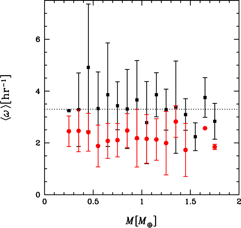
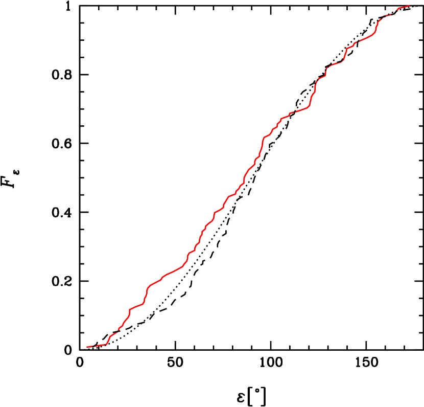
Figure 3: Left: Average spin angular velocity of all planets formed in the 50 runs of the realistic (circle) and perfect (square) accretion models is plotted against their mass $M$ with mass bin of 0.1$M_{\oplus}$. The error bars indicate 1-$\sigma$ and the dotted line shows $\omega_{\rm cr}$. Right: Normalized cumulative distributions of $\varepsilon$ for the realistic (solid curve) and perfect (dashed curve) accretion models with an isotropic distribution (dotted curve).

Table 1: Basic Dynamical Properties of Final Planets

accretion model	$\langle n\rangle$	$\langle n_{M}\rangle$	$\langle n_{a}\rangle$	$\langle f_{a}\rangle$	$\langle T_{\rm grow}\rangle$($10^{8}$ yr)	$\langle n_{\rm har}\rangle$	$\langle n_{\rm acc}\rangle$	$\langle M_{1}\rangle$($M_{\oplus}$)	$\langle a_{1}\rangle({\rm AU})$	$\langle e_{1}\rangle$	$\langle i_{1}\rangle$	$\langle M_{2}\rangle$($M_{\oplus}$)	$\langle a_{2}\rangle({\rm AU})$	$\langle e_{2}\rangle$	$\langle i_{2}\rangle$
realistic	3.6$\pm$0.8	2.0$\pm$0.5	1.6$\pm$0.6	0.63$\pm$0.2	0.73$\pm$0.74	11.8$\pm$7.7	12.4$\pm$0.8	1.18$\pm$0.23	0.79$\pm$0.27	0.12$\pm$0.07	0.07$\pm$0.05	0.72$\pm$0.20	0.91$\pm$0.50	0.15$\pm$0.07	0.10$\pm$0.05
perfect	3.1$\pm$0.6	2.0$\pm$0.6	1.7$\pm$0.6	0.77$\pm$0.2	0.60$\pm$0.71	$\cdots$	12.9$\pm$0.6	1.26$\pm$0.25	0.77$\pm$0.24	0.12$\pm$0.06	0.06$\pm$0.04	0.72$\pm$0.23	0.97$\pm$0.52	0.14$\pm$0.08	0.09$\pm$0.06

Table 2: Spin Parameters of Final Planets

accretion model	$\langle\omega_{x}\rangle$(${\rm hr}^{-1}$)	$\langle\omega_{y}\rangle$(${\rm hr}^{-1}$)	$\langle\omega_{z}\rangle$(${\rm hr}^{-1}$)	$\sigma_{x}$(${\rm hr}^{-1}$)	$\sigma_{y}$(${\rm hr}^{-1}$)	$\sigma_{z}$(${\rm hr}^{-1}$)	$\langle\omega^{2}\rangle^{1/2}$(${\rm hr}^{-1}$)	$\beta$
realistic	0.05	0.08	0.07	1.32	1.26	1.49	2.35	0.40
perfect	0.42	-0.09	-0.16	2.15	2.17	2.03	3.69	0.31

References

- Agnor & Asphaug (2004) Agnor, C., & Asphaug, E. 2004, ApJ, 613, L157
- Agnor et al. (1999) Agnor, C. B., Canup, R. M., & Levison, H. F. 1999, Icarus, 142, 219
- Canup (2004) Canup, R. M. 2004, Icarus, 168, 433
- Chambers (2001) Chambers, J. E. 2001, Icarus, 152, 205
- Hayashi (1981) Hayashi, C. 1981, Prog. Theor. Phys. Suppl., 70, 35
- Ida & Makino (1992) Ida, S., & Makino, J. 1992, Icarus, 96, 107
- Kokubo & Ida (1998) Kokubo, E., & Ida, S. 1998, Icarus, 131, 171
- Kokubo & Ida (2000) Kokubo, E., & Ida, S., 2000, Icarus, 143, 15
- Kokubo & Ida (2002) Kokubo, E., & Ida, S., 2002, ApJ, 581, 666
- Kokubo et al. (2006) Kokubo, E., Kominami, J., & Ida, S., 2006, ApJ, 642, 1131
- Kokubo & Ida (2007) Kokubo, E., & Ida, S., 2007, ApJ, 671, 2082
- Kokubo & Makino (2004) Kokubo, E., & Makino, J. 2004, PASJ, 56, 861
- Kokubo et al. (1998) Kokubo, E., Yoshinaga, K., & Makino, J. 1998, MNRAS, 297, 1067
- Kominami & Ida (2002) Kominami, J., & Ida, S. 2002, Icarus, 157, 43
- Makino (1991) Makino, J. 1991, PASJ, 43, 859
- Melosh (1989) Melosh, H. J. 1989, Impact Cratering: A Geologic Process (New York: Oxford Univ. Press)
- Monaghan (1992) Monaghan, J. J. 1992, ARA&A, 30, 543
- Nitadori et al. (2006) Nitadori, K., Makino, J., & Hut, P. 2006, New Astronomy, 12, 169.
- Wetherill (1985) Wetherill, G. W. 1985, Science, 228, 877