One-loop contribution to the neutrino mass matrix in NMSSM with right-handed neutrinos and tri-bimaximal mixing

Abstract

Neutrino mass patterns and mixing have been studied in the context of next-to-minimal supersymmetric standard model (NMSSM) with three gauge singlet neutrino superfields. We consider the case with the assumption of R-parity conservation. The vacuum expectation value of the singlet scalar field $S$ of NMSSM induces the Majorana masses for the right-handed neutrinos as well as the usual $\mu$-term. The contributions to the light neutrino mass matrix at the tree level as well as one-loop level are considered, consistent with the tri-bimaximal pattern of neutrino mixing. Light neutrino masses arise at the tree level through a TeV scale seesaw mechanism involving the right-handed neutrinos. Although all the three light neutrinos acquire non-zero masses at the tree-level, we show that the one-loop contributions can be comparable in size under certain conditions. Possible signatures to probe this model at the LHC and its distinguishing features compared to other models of neutrino mass generation are briefly discussed.

I Introduction

Several mechanisms of the generation of neutrino masses and mixing in the context of a supersymmetric model have been explored in various works. One of the most popular attempts in this direction is to relax the assumption of R-parity conservation in the minimal supersymmetric standard model (MSSM) by including explicit bilinear and/or trilinear R-parity violating interactions in the superpotential and the scalar potentialr-parity-early-references ; r-parity-review . One can also consider models with spontaneous R-parity violation romao-santos-valle ; giudice-masiero-pietroni-riotto ; umemura-yamamoto via a singlet sneutrino vacuum expectation value. The low energy limit of such models, where the singlet sneutrino field is decoupled, can be thought of as the bilinear R-parity violating scenario. Thus there are several possibilities within the context of R-parity violation in MSSM. In fact, each of them has been studied in detail in connection with the observed neutrino mass patterns and mixing as provided by the neutrino oscillation experiments. The possible collider signatures of R-parity violating models have also been studied in great details and correlation between neutrino mixing angles and the decay branching ratios of the lightest supersymmetric particle (LSP) have been obtained gonzalez-garcia-romao-valle ; adhikari-mukhopadhyaya ; hirsch-vicente-porod ; Roy-Mukhopadhyaya-Vissani ; choi-chun-kang-lee ; romao-diaz-hirsch-porod-valle ; datta-mukhopadhyaya-vissani ; porod-hirsch-romao-valle ; chun-jung-kang-park ; jung-kang-park-chun .

Another interesting and well studied procedure of small neutrino mass generation in a supersymmetric model, with the observed mixing pattern, is the seesaw mechanismoriginal-seesaw ; other-early-seesaw with the introduction of right-handed neutrino superfieldsgrossman-haber ; susy-seesaw ; davidson-king . In order to generate small neutrino masses, one introduces $\Delta L$ = 2 heavy Majorana mass terms in the superpotential in addition to the trilinear lepton-number conserving Yukawa interactions involving the right-handed neutrino superfields. As long as the neutrino Yukawa couplings are of order one, light neutrino masses $\sim 10^{-2}$ eV require the Majorana masses to be $\sim 10^{15}$ GeV or so. However, such a high seesaw scale is difficult to probe at the LHC or future linear collider experiments. A viable alternative is to look at TeV-scale seesaw mechanism where small active neutrino masses are generated with the help of neutrino Yukawa couplings as small as $10^{-6}$ (same as the electron Yukawa coupling) and this makes the Majorana mass scale of the right-handed neutrino of the order of $\sim$ TeV plausible. This gives one an opportunity to test the seesaw models at the LHC. The signatures of TeV scale supersymmetric seesaw models will be briefly outlined later along with a discussion of the signatures of R-parity-violating models.

On the other hand, MSSM is plagued by the so-called “$\mu$-problem” which asks the question that why the scale of the supersymmetry preserving $\mu$-term should be of the same order as the soft supersymmetry breaking terms, which are of the order of TeV. One of the possible solutions to this problem is the next-to-minimal supersymmetric standard model (NMSSM), where a standard model singlet superfield ($\hat{S}$) is introduced to the MSSM superfields with a coupling $\lambda{\hat{S}}{\hat{H}}_{u}{\hat{H}}_{d}$ in the superpotential (for review and phenomenology seeNMSSM_review1 ; NMSSM_review2 ). The scalar component of ${\hat{S}}$ gets, in general, a non-zero vacuum expectation value (VEV) of the order of $\sim$ TeV, as long as the soft mass parameters corresponding to the singlet scalar field are in the same range. This solves the “$\mu$-problem” because the $\mu$-parameter generated in this way has the right order of magnitude if one considers a coupling $\lambda\sim{\cal O}(1)$. In order to generate active neutrino masses and appropriate mixing in the neutrino sector one either includes R-parity violation in the superpotentialchemtob-pandita ; abada-bhattacharyya-moreau and the scalar potential or introduces gauge-singlet neutrino superfields $\hat{N}_{i}$ with appropriate couplings with the MSSM superfields and the singlet superfield ${\hat{S}}$Kitano-2001 . In the latter case, the gauge-singlet neutrino superfields $\hat{N}_{i}$ can have Majorana masses around the TeV scale if there is a coupling of the type $\kappa\hat{N}_{i}^{2}\hat{S}$ in the superpotential. When the scalar component of ${\hat{S}}$ gets a VEV of the order of TeV scale, the right handed neutrinos also acquire an effective Majorana mass around the TeV values as long as the dimensionless coupling $\kappa$ is order oneKitano-2001 . Here it is assumed that the superpotential has a discrete $Z_{3}$ symmetry which forbids the appearance of bilinear terms in the superpotential ellis89 .

In this study, within the framework of this TeV scale seesaw model mentioned above, we calculate the one-loop contributions to the neutrino mass matrix with R-parity conservation and study the effect of these contributions to the neutrino mass patterns and mixing angles. In other words, we consider the case where only the scalar field corresponding to the singlet superfield $\hat{S}$ gets a non-zero VEV along with the neutral Higgs fields. We will show later that these one-loop contributions can be significant and can change the region of parameter space allowed by the three-flavor global neutrino data in comparison to the tree level results.

The plan of the paper is as follows. In Sec.II we will provide a discussion on the three-flavor neutrino mixing and illustrate the general pattern of our analysis that we are going to follow. Sec.III describes the model along with the minimization conditions of the neutral scalar potential. One-loop contributions to the neutrino mass matrix in the R-parity conserving scenario and the resulting neutrino mass patterns, which satisfy the three flavor global neutrino data, are discussed in Sec.IV with numerical results. In Sec.V we outline the possible ways to probe this model at the LHC and present a short critical discussion of the signatures of neutrino mass models involving spontaneous and/or bilinear R-parity violation. We summarize in Sec.VI with possible future directions.

II Neutrino mixing

The solar, atmospheric, accelerator, and reactor neutrino experiments have shown strong evidence in favor of non-zero neutrino masses and mixing anglesStrumia . In addition, there is an upper bound on the sum of neutrino mass eigenvalues $\sim$1 eV from cosmological observationsneutrino_sum . The bound on the 11-element of the neutrino mass matrix resulting from the non-observation of neutrinoless double beta decay is $\leq$0.3 eVneutrino_mass . The global 3-flavor fits of various neutrino oscillation experiments point toward the following 3$\sigma$ ranges of the neutrino oscillation parameters, namely the two mass-squared differences and three mixing anglesnew-neu-recent-data :

$$\sin^{2}\theta_{12}=0.25-0.37,\ \sin^{2}\theta_{23}=0.36-0.67,$$

$$\sin^{2}\theta_{13}\leq 0.056$$

$$\Delta m_{21}^{2}=(7.05-8.34)\times 10^{-5}\;{\rm eV}^{2}\;,$$

$$|\Delta m_{31}^{2}|=(2.07-2.75)\times 10^{-3}\;{\rm eV}^{2}\;,$$ (1)

where $\Delta m^{2}_{ij}\equiv m^{2}_{i}-m^{2}_{j}$. One can see from these numbers that there are two large mixing angles and one small mixing angle among the three light neutrinos with a mild hierarchy between the mass eigenvalues.

The three flavor neutrino mixing matrix $U$ can be parametrized as follows, provided that the charged lepton mass matrix is already in the diagonal form and the Dirac as well as Majorana phases are neglected:

$$U=\left(\begin{array}[]{ccc}c_{12}c_{13}&s_{12}c_{13}&s_{13}\\ -s_{12}c_{23}-c_{12}s_{23}s_{13}&c_{12}c_{23}-s_{12}s_{23}s_{13}&s_{23}c_{13}\\ s_{12}s_{23}-c_{12}c_{23}s_{13}&-c_{12}s_{23}-s_{12}c_{23}s_{13}&c_{23}c_{13}\end{array}\right),\hskip-22.76228pt$$ (5)

where $c_{ij}=\cos\theta_{ij}$, $s_{ij}=\sin\theta_{ij}$ and $i,j$ run from 1 to 3.

The mixing angle data coming from solar, atmospheric and reactor sector indicate that $\theta_{12}\approx 34^{\circ}$, $\theta_{23}\approx 45^{\circ}$, and $\theta_{13}\leq 13^{\circ}$. This is popularly known as the bilarge pattern of neutrino mixing. In order to understand the consequences of such mixing in the zeroth order, one considers the tri-bimaximal structure of the neutrino mixinghps where $\theta_{23}=\frac{\pi}{4}$, $\theta_{13}=0$ and $\sin\theta_{12}=\frac{1}{\sqrt{3}}$.

With this tri-bimaximal pattern, the unitary neutrino mixing matrix turns out to be

$$U_{\nu}=\left(\begin{array}[]{ccc}\sqrt{\frac{2}{3}}&\frac{1}{\sqrt{3}}&0\\ -\frac{1}{\sqrt{6}}&\frac{1}{\sqrt{3}}&\frac{1}{\sqrt{2}}\\ \frac{1}{\sqrt{6}}&-\frac{1}{\sqrt{3}}&\frac{1}{\sqrt{2}}\end{array}\right).$$ (7)

Considering $m_{1}$, $m_{2}$ and $m_{3}$ as the three light neutrino mass eigenvalues, we use the matrix $U_{\nu}$ to obtain the neutrino Majorana mass matrix in the flavor basis as

$$m_{\nu} = U_{\nu}\left(\begin{array}[]{ccc}m_{1}&&\\ &m_{2}&\\ &&m_{3}\end{array}\right)U^{T}_{\nu}$$ (11)

$$= \left(\begin{array}[]{ccc}\frac{1}{3}(2m_{1}+m_{2})&\frac{1}{3}(-m_{1}+m_{2})&\frac{1}{3}(m_{1}-m_{2})\\ \frac{1}{3}(-m_{1}+m_{2})&\frac{1}{6}(m_{1}+2m_{2}+3m_{3})&\frac{1}{6}(-m_{1}-2m_{2}+3m_{3})\\ \frac{1}{3}(m_{1}-m_{2})&\frac{1}{6}(-m_{1}-2m_{2}+3m_{3})&\frac{1}{6}(m_{1}+2m_{2}+3m_{3})\end{array}\right).$$ (15)

We can see that a particular structure of neutrino mass matrix emerges from the requirement of tri-bimaximal mixing, in terms of the neutrino mass eigenvalues. Given a specific model for generating the neutrino mass matrix, one can easily connect the model parameters with the neutrino mass eigenvalues with the help of Eq.(15). This way one can study the normal, inverted or quasi-degenerate mass pattern of the light neutrino mass eigenvalues and try to see the requirement on the model parameters to produce the tri-bimaximal pattern of neutrino mixing. In this work, we will try to explore the next-to-minimal supersymmetric standard model (NMSSM) where neutrino mass is generated because of the introduction of three right-handed neutrino superfields with the possible interaction terms. Though the assumption of tri-bimaximal mixing in the neutrino sector is not generic, in the present context it is quite illustrative in studying the role of the soft SUSY breaking parameters on the neutrino mass eigenvalues. At the same time, the acceptable domain of the soft parameters consistent with neutrino mass eigenvalues and tri-bimaximal mixing angles would hardly change with any small shift in $\theta_{13}$.

As mentioned in the introduction, this model was proposed in Ref.Kitano-2001 where the case with spontaneous violation of R-parity was studied with possible implications on neutrino mass eigenvalues and mixing angles at the tree level. In the present study we shall consider the case when R-parity is conserved and the neutrino mass generation at the tree level is entirely due to the seesaw mechanism involving the TeV scale right handed neutrinos. Our aim would be to see if this model can produce the acceptable neutrino mass eigenvalues and mixing angles when the neutrino mass matrix receives contributions at the tree as well as one-loop level. An attractive feature of this model is that, the right handed sneutrino in the form of LSP may become a valid cold dark matter candidate of the universecerdenoall .

This model can also accommodate spontaneous CP and R-parity violation simultaneously. In that case, the neutrino sector is CP violating and the resulting effects on the neutrino masses and mixing angles were studied in Ref.katri-mariana-timo . Similarly, spontaneous R-parity violation motivated by a flavor symmetry may produce tri-bimaximal mixing pattern in the neutrino sectormanimala . However, in the present context we consider the case where neutrino sector conserves CP symmetry along with R-parity.

There have been some other studies which address the neutrino experimental data in some other extensions of NMSSM. One of these proposals is discussed in Ref.chemtob-pandita , where the effective bilinear R-parity breaking terms are generated through the vacuum expectation value of the scalar component of the singlet superfield ${\hat{S}}$. In this case, only one neutrino mass is generated at the tree level whereas the other two masses are generated at the one-loop level. In another modelabada-bhattacharyya-moreau , non-zero masses for two neutrinos are generated at the tree level by including explicit bilinear R-parity violating terms along with the R-parity breaking term involving ${\hat{S}}$. It is interesting to note that, the R-parity violating NMSSM model may offer a valid dark matter candidate in the form of gravitino as the R-parity violating decay channels of the gravitino are extremely suppressed because of weak gravitational strengthmoreau-dark .

In another class of models, gauge-singlet neutrino superfields were introduced to solve the $\mu$-problem, which can simultaneously address the desired pattern of neutrino masses and mixingmunoz . The detailed study of neutrino masses and mixing in this model was presented in Ref.ghosh-roy and the correlations of the lightest neutralino decays with neutrino mixing angles were discussed. Subsequently the dominant one-loop contributions towards the tree level neutrino masses have also been presentedghosh-roy-loop . Similar analyses for one and two generations of gauge-singlet neutrinos were presented in Ref.hirsch-vicente and some other phenomenological implications, in particular the possible signatures at LHC were addressed. Neutrino masses consistent with different hierarchical scenarios and tri-bimaximal neutrino mixing can also be generated in an R-parity violating supersymmetric theory with TeV scale gauge singlet neutrino superfields, where the $\mu$-term was not generated by the vacuum expectation values of the singlet sneutrino fields Mukhopadhyaya:2006is . Another interesting avenue in this direction is to study the role of possible higher dimensional supersymmetry breaking operators in the hidden sector which may render the TeV scale soft SUSY breaking trilinear and bilinear couplings involving the sneutrinos to produce the observable mass and mixing angles for the neutrinoshigher-dimension .

III The model and minimization conditions

In this section we review the model along the lines of Ref.Kitano-2001 and discuss its important characteristics. We introduce the singlet superfield $\hat{S}$ along with three right-handed neutrino superfields $\hat{N}_{i}$. The superfields $\hat{N}_{i}$ are odd and the superfield $\hat{S}$ is even under R-parity. The most general superpotential consistent with R-parity conservation is

$$W = W_{\rm NMSSM}+W_{\it Singlet}\ ,$$ (16)

where

$$W_{\rm NMSSM} = f^{d}_{i}(\hat{H}_{d}\hat{Q}_{i})\hat{D}_{i}+f^{u}_{ij}(\hat{Q}_{i}\hat{H}_{u})\hat{U}_{j}$$ (17)

$$+ f^{e}_{i}(\hat{H}_{d}\hat{L}_{i})\hat{E}_{i}+\lambda_{H}(\hat{H}_{d}\hat{H}_{u})\hat{S}+\frac{\lambda_{s}}{3!}\hat{S}^{3}\ ,$$

$$W_{\it Singlet} = f^{\nu}_{ij}(\hat{L}_{i}\hat{H}_{u})\hat{N}_{j}+\frac{{\lambda_{N}}_{i}}{2}\hat{N}_{i}^{2}\hat{S}.$$ (18)

Here $\hat{H}_{d}$ and $\hat{H}_{u}$ are down-type and up-type Higgs superfields, respectively. The $\hat{Q}_{i}$ are doublet quark superfields, $\hat{U}_{j}[\hat{D}_{j}]$ are singlet up-type [down-type] quark superfields. The $\hat{L}_{i}$ are the doublet lepton superfields, and the $\hat{E}_{j}$ are the singlet charged lepton superfields. The indices $i,j=1,2,3$ are generation indices. Note that we have imposed a $Z_{3}$ symmetry under which all the superfields have the same charge. This symmetry forbids the appearance of the usual bilinear $\mu$-term in the superpotential. The $\mu$-term is generated spontaneously through the vacuum expectation value of the singlet scalar $\hat{S}$. In a similar way soft supersymmetry breaking potential can be written as

$$V_{\rm soft}=V_{\rm soft}^{\rm NMSSM}+V_{\it Singlet}\ ,$$ (19)

where $V_{\rm soft}^{\rm NMSSM}$ includes the MSSM soft supersymmetry breaking terms along with a few additional terms as shown below:

$$V_{\rm soft}^{\rm NMSSM}=V_{\rm soft}^{\rm MSSM}+m_{S}^{2}|S|^{2}+$$

$$\mbox{}\left(A^{H}\lambda_{H}H_{d}H_{u}S+Am\frac{\lambda_{s}}{3!}S^{3}+\rm H.c\right).$$ (20)

The term $V_{\it Singlet}$ is composed of the soft masses and the trilinear interactions corresponding to the fields $\tilde{N}_{i}$:

$$V_{\it Singlet}=m^{2}_{{\tilde{N}}{\tilde{N}}^{*}}|\tilde{N}_{i}|^{2}+$$

$$\mbox{}\left(A^{\nu}f^{\nu}_{ij}\tilde{L}_{i}H_{u}\tilde{N}_{j}+Am\frac{\lambda_{Ni}}{2}S\tilde{N}_{i}^{2}+\rm H.c\right).$$ (21)

We have taken a common trilinear coupling $A$ for the singlet fields $N_{i}$ and $S$ and $m$ is a mass scale. In a supergravity motivated scenario, it is a common practice to choose $m=m_{S}=m_{{\tilde{N}}{\tilde{N}}^{*}}$ and also a universal trilinear parameter for the fields $S$, $\tilde{N}_{i}$. Since these fields are gauge singlet, we assume such universality to hold also at the electroweak scale. Similarly, the mass parameters $m_{S}$ and $m_{{\tilde{N}}{\tilde{N}}^{*}}$ are very much insensitive to Renormalization Group Equation (RGE) running and their values at the weak scale can be taken to be the same as the values at the high scale. In addition, we have chosen all the parameters $f^{d}_{i}$, $f^{e}_{i}$, ${\lambda_{N}}_{i}$, $\lambda_{H}$, $\lambda_{s}$,$f^{u}_{ij}$ and $f^{\nu}_{ij}$ to be real.

The scalar potential of this model can be written as

$$V=V_{F}+V_{D}+V_{\rm soft}\ ,$$ (22)

where the neutral part of $V_{F}$ and $V_{D}$ can be written as

$$V^{\it neutral}_{F} = \sum_{i}\left|f^{\nu}_{ij}H^{0}_{u}\tilde{N}_{j}\right|^{2}+\left|\lambda_{H}H^{0}_{u}S\right|^{2}+\left|f^{\nu}_{ij}\tilde{\nu}_{i}\tilde{N}_{j}+\lambda_{H}H^{0}_{d}S\right|^{2}$$ (23)

$$+\sum_{j}\left|f^{\nu}_{ij}(\tilde{\nu}_{i}H^{0}_{u})+{\lambda_{N}}_{j}\tilde{N}_{j}S\right|^{2}+\left|\lambda_{H}(H^{0}_{d}H^{0}_{u})+\frac{{\lambda_{N}}_{i}}{2}\tilde{N}_{i}^{2}+\frac{\lambda_{s}}{2}S^{2}\right|^{2},$$

$$V_{D}^{\it neutral} = \frac{g_{1}^{2}+g_{2}^{2}}{8}\left(|H_{u}^{0}|^{2}-|H_{d}^{0}|^{2}-\sum_{i}|\tilde{\nu}_{i}|^{2}\right)^{2}\ .$$ (24)

In the above, the repeated indices always mean to sum over the generations. However, the summation sign is used in special cases if required. The VEVs are determined by the minimization of the potential (vide Eq.(22), (23) and (24)). Here we explore the possibility when only scalar component of the gauge singlet superfield $\hat{S}$ acquires a VEV along with the doublet Higgs fields. The right-chiral sneutrino $\tilde{N}$ can only have a vanishing VEV and thus R-parity is unbroken. On the other hand, when the right-chiral sneutrino ${\tilde{N}}$ acquires a VEV then R-parity is spontaneously broken and an effective bilinear R-parity violating term of the form $\epsilon_{i}L_{i}H_{u}$ is generated, where $\epsilon_{i}\equiv f^{\nu}\langle\tilde{N}_{i}\rangle$. However, the case of spontaneous R-parity violation will be studied in a separate workdebottam-future . Note that, a global continuous symmetry such as lepton number cannot be assigned to the superpotential involving the singlets $\hat{S}$ and $\hat{N}_{i}$. Thus this model is completely free from the unwanted Nambu-Goldstone boson even if the singlet scalar $S$ and/or $\tilde{N}_{i}$ acquire VEV. For more details the reader is referred to Ref.tev-seesaw ; Kitano-2001 .

Minimization of the scalar potential (vide Eq.(22)) leads to the following conditions$\colon$

$${\partial V\over\partial v_{d}} = 2v_{d}(m_{H_{d}}^{2}+\lambda_{H}^{2}(v_{u}^{2}+v_{s}^{2})+{g_{1}^{2}+g_{2}^{2}\over 4}(v_{d}^{2}-v_{u}^{2}+\sum_{i}v_{\tilde{\nu}_{i}}^{2})$$

$$+ \tan\beta({1\over 2}\lambda_{H}\lambda_{s}v_{s}^{2}+{1\over 2}\lambda_{H}\lambda_{N_{i}}v_{\tilde{N}_{i}}^{2}+A_{H}\lambda_{H}v_{s}))+2\lambda_{H}f_{\nu}^{ij}v_{s}v_{\tilde{\nu}_{i}}v_{\tilde{N}_{j}},$$

$${\partial V\over\partial v_{u}} = 2v_{u}(m_{H_{u}}^{2}+\lambda_{H}^{2}(v_{d}^{2}+v_{s}^{2})-{g_{1}^{2}+g_{2}^{2}\over 4}(v_{d}^{2}-v_{u}^{2}+\sum_{i}v_{\tilde{\nu}_{i}}^{2})$$

$$+ f_{\nu}^{ij}f_{\nu}^{ik}v_{\tilde{N}_{j}}v_{\tilde{N}_{k}}+f_{\nu}^{ji}f_{\nu}^{ki}v_{\tilde{\nu}_{j}}v_{\tilde{\nu}_{k}}+\cot\beta({1\over 2}\lambda_{H}\lambda_{s}v_{s}^{2}+{1\over 2}\lambda_{H}\lambda_{N_{i}}v_{\tilde{N}_{i}}^{2}+A_{H}\lambda_{H}v_{s}))$$

$$+ 2A_{\nu}f_{\nu}^{ij}v_{\tilde{\nu}_{i}}v_{\tilde{N}_{j}}+2f_{\nu}^{ji}\lambda_{N_{i}}v_{s}v_{\tilde{\nu}_{j}}v_{\tilde{N}_{i}},$$

$${\partial V\over\partial v_{s}} = 2v_{s}(m_{S}^{2}+\lambda_{H}^{2}(v_{d}^{2}+v_{u}^{2})+\lambda_{s}\lambda_{H}v_{d}v_{u}+\lambda_{N_{i}}^{2}v_{\tilde{N}_{i}}^{2}+{1\over 2}Am\lambda_{s}v_{s}+{1\over 2}\lambda_{s}^{2}v_{s}^{2}+{1\over 2}\lambda_{s}\lambda_{N_{i}}v_{\tilde{N}_{i}}^{2})$$

$$+ 2A_{H}\lambda_{H}v_{d}v_{u}+Am\lambda_{N_{i}}v_{\tilde{N}_{i}}^{2}+2f_{\nu}^{ij}v_{\tilde{\nu}_{i}}v_{\tilde{N}_{j}}(\lambda_{H}v_{d}+\lambda_{N_{j}}v_{u}),$$

$${\partial V\over\partial v_{\tilde{\nu}_{i}}} = 2v_{\tilde{\nu}_{i}}({\tilde{m}}^{2}_{i}+{g_{1}^{2}+g_{2}^{2}\over 4}(v_{d}^{2}-v_{u}^{2}+\sum_{j}v_{\tilde{\nu}_{j}}^{2}))+2A_{\nu}f_{\nu}^{ij}v_{u}v_{\tilde{N}_{j}}$$

$$+ 2\lambda_{H}f_{\nu}^{ij}v_{d}v_{s}v_{\tilde{N}_{j}}+2f_{\nu}^{ik}f_{\nu}^{jk}v_{u}^{2}v_{\tilde{\nu}_{j}}+2f_{\nu}^{ij}\lambda_{N_{j}}v_{u}v_{s}v_{\tilde{N}_{j}}+2f_{\nu}^{ij}f_{\nu}^{kl}v_{\tilde{N}_{j}}v_{\tilde{\nu}_{k}}v_{\tilde{N}_{l}},$$

$${\partial V\over\partial v_{\tilde{N}_{i}}} = 2v_{\tilde{N}_{i}}(m^{2}_{{\tilde{N}}{\tilde{N}}^{*}}+Am\lambda_{N_{i}}v_{s}+\lambda_{N_{i}}\lambda_{H}v_{d}v_{u}+\frac{1}{2}\lambda_{N_{i}}\lambda_{s}v_{s}^{2}+\lambda_{N_{i}}^{2}v_{s}^{2}+\frac{1}{2}\lambda_{N_{i}}\lambda_{N_{j}}v_{\tilde{N}_{j}}^{2})$$

$$+ 2f_{\nu}^{ji}f_{\nu}^{jk}v_{u}^{2}v_{\tilde{N}_{k}}+2A_{\nu}f_{\nu}^{ji}v_{u}v_{\tilde{\nu}_{j}}+2\lambda_{H}f_{\nu}^{ji}v_{d}v_{s}v_{\tilde{\nu}_{j}}+2\lambda_{N_{i}}f_{\nu}^{ji}v_{u}v_{s}v_{\tilde{\nu}_{j}}+2f_{\nu}^{ji}f_{\nu}^{kl}v_{\tilde{\nu}_{j}}v_{\tilde{N}_{l}}v_{\tilde{\nu}_{k}}.$$

Here $g_{1}$ and $g_{2}$ are the U(1) and SU(2) gauge couplings, respectively, and $\tan\beta=v_{u}/v_{d}$. ${\tilde{m}}_{i}$ is the soft SUSY breaking mass parameter of the left chiral sneutrinos. We have assumed that the neutral scalar fields can develop, in general, the following vacuum expectation values

$$v_{d} = \langle H^{0}_{d}\rangle;\hskip 5.69046ptv_{u}=\langle H^{0}_{u}\rangle;\hskip 5.69046ptv_{s}=\langle S\rangle;\hskip 5.69046pt$$

$$v_{\tilde{\nu}_{i}} = \langle\tilde{\nu}_{i}\rangle;\hskip 5.69046ptv_{\tilde{N}_{i}}=\langle\tilde{N}_{i}\rangle.$$ (26)

As has already been mentioned, in the present context we will consider the solutions $v_{\tilde{N}_{i}}=v_{\tilde{\nu}_{i}}=0$ and $v_{s}\neq 0$ to analyze the neutrino spectra. In our subsequent discussion, we will also ignore the terms in the minimization equations which are bilinear in the neutrino Yukawa couplings. Note that in order to generate very small masses for the active neutrinos ($\ {}^{<}\hbox to0.0pt{\hss${}_{\sim}$}\$0.1 eV) using this TeV scale seesaw mechanism, the neutrino Yukawa couplings ($f^{\nu}$) should be below ${\cal O}(10^{-6})$, which is around the magnitude of the electron Yukawa coupling.

The VEV $v_{s}$ comes out as the solution of the following cubic equation (neglecting the Yukawa term),

$$\hskip-17.07182pt\lambda_{s}^{2}v_{s}^{3}+Am\lambda_{s}v_{s}^{2}+2v_{s}(m_{s}^{2}+\lambda_{H}^{2}v_{u}^{2}+\lambda_{H}^{2}v_{d}^{2}+\lambda_{H}\lambda_{s}v_{d}v_{u}$$

$$+ \hskip-4.26773pt\lambda^{2}_{N_{i}}v_{\tilde{N}_{i}}^{2}+\lambda_{s}\lambda_{N_{i}}v_{\tilde{N}_{i}}^{2})+2A_{H}\lambda_{H}v_{d}v_{u}+Am\lambda_{N_{i}}v_{\tilde{N}_{i}}^{2}=0.$$

The solutions of the foregoing equation involve soft parameters $Am$, $A_{H}$ and $m_{s}^{2}$. In fact these parameters cannot be much away from TeV values to have $v_{s}$ $\sim$ TeV. In particular, the soft parameter $A_{H}$ and $Am$ are crucial to produce non zero VEV for the field $S$. Any consistent solution that yields $v_{s}\neq 0$ but $v_{\tilde{N}_{i}}=0$ requires $|A|\geq 3$ and also $\lambda_{H}\leq 1$, $m\geq 100$ GeV, $m_{S}\geq 100$ GeVKitano-2001 . Similarly we also choose the couplings $\lambda_{s}$, $\lambda_{N_{i}}$ in such a manner so that the condition for global minima is always satisfied.

IV Neutrino masses and mixing: R-parity conserving NMSSM

Let us now discuss in detail the generation of neutrino masses and mixing in this model. Note that this model is different from the models where MSSM is extended with three right-handed singlet neutrino superfields. This is because in those models the right handed neutrino mass scale is not tied up with the electroweak symmetry breaking scale and is assumed to be very high ($\sim 10^{15}$ GeV or so).

IV.1 Seesaw masses

At the tree level, the $(3\times 3)$ light neutrino mass matrix, that arises via the seesaw mechanism has a very well-known structure given by

$$m_{\nu}^{tree}=-m_{D}M^{-1}_{R}m^{T}_{D},$$ (28)

where $m_{D}$ represents the lepton number conserving $(3\times 3)$ ‘Dirac’ mass matrix and $M_{R}$ represents the lepton number violating $(3\times 3)$ ‘Majorana’ mass matrix. Note that, after the EWSB, when the scalar component of ${\hat{S}}$ gets a VEV, in the effective Lagrangian we can assign a lepton number -1 for the fields $N_{i}^{c}$ and ${\tilde{N}}_{i}$ (contained in the superfield ${\hat{N}}_{i}$). The relevant part of the effective Lagrangian which encompasses both neutrino and sneutrino fields is given by

$$-{\cal L}_{eff} = \frac{1}{2}(\lambda_{Ni}v_{s}){N^{c}_{i}}{N^{c}_{i}}+f^{\nu}_{ij}{\nu_{i}}{v_{u}}{N^{c}_{j}}+\rm H.c.$$

$$+ m^{2}_{\tilde{\nu}_{i}}{\tilde{\nu}_{i}}{\tilde{\nu}^{\star}_{i}}+(m_{\tilde{N}_{i}{\tilde{N}_{i}}^{*}}^{2}+\lambda_{N_{i}}^{2}v_{s}^{2}){\tilde{N}_{i}}{\tilde{N}^{\star}_{i}}$$

$$+ (B^{\nu}_{ij}{\tilde{\nu}_{i}}{\tilde{N}_{j}}+{B^{{\prime}\nu}_{ij}}{\tilde{\nu}_{i}}{\tilde{N}^{\star}_{j}}+B_{Ri}{\tilde{N}_{i}}{\tilde{N}_{i}}+{\rm H.c.}),$$

where the coefficients have the following meaning

$$m^{2}_{\tilde{\nu}_{i}} = {\tilde{m}}^{2}_{i}+\frac{1}{2}m_{Z}^{2}cos2\beta,$$

$$B^{\nu}_{ij} = A^{\nu}f^{\nu}_{ij}{v_{u}}+\lambda_{H}f^{\nu}_{ij}v_{d}v_{s},$$

$$B^{{\prime}\nu}_{ij} = f^{\nu}_{ij}\lambda_{Nj}{v_{u}}{v_{s}},$$

$$B_{Ri} = \frac{1}{2}({\lambda_{H}\lambda_{N_{i}}v_{d}v_{u}}+\frac{\lambda_{s}\lambda_{N_{i}}v_{s}^{2}}{2}+Am\lambda_{Ni}{v_{s}}).$$

It is easy to see from Eq.(LABEL:eq-eff-lagrangian) that ${m_{D}}_{ij}\equiv f^{\nu}_{ij}v_{u}$ and $M_{R}{{}_{i}}=\lambda_{Ni}v_{s}$, which in turn provide neutrino masses at the tree level through Eq.(28). Note that, in Eq.(LABEL:loopcoeff1) we have neglected a term $\sim m^{2}_{D}$ in the expression for $m^{2}_{\tilde{\nu}_{i}}$ since it is much smaller compared to the other terms.

The tree level neutrino masses may receive dominant radiative corrections at the one-loop level. It has been shown in models of MSSM with right-handed neutrino superfields, that the loop contributions can be as large as the tree level value, though the result depends on the soft SUSY breaking parameters grossman-haber ; davidson-king . In $R$-parity conserving scenarios the leading contribution to neutrino masses at the one-loop level arise from $\Delta L=2$ terms in the sneutrino sector. These bilinear interaction terms involving the heavy right-handed sneutrinos fields ${\tilde{N}}_{i}$ are ${B^{{\prime}\nu}_{ij}}{\tilde{\nu}_{i}}{\tilde{N}^{\star}_{j}}$, and $B_{Ri}{\tilde{N}_{i}}{\tilde{N}_{i}}$ as can be seen from Eq.(LABEL:eq-eff-lagrangian). In association with the $\Delta L=0$ term i.e., $B^{\nu}_{ij}{\tilde{\nu}_{i}}{\tilde{N}_{j}}$ these $\Delta L=2$ terms generate lepton number violating “Majorana” like mass terms ($m^{2}_{{\tilde{\nu}}{\tilde{\nu}}}{\tilde{\nu}}{\tilde{\nu}}+h.c.$) for the left-handed sneutrinos. In fact, this can be seen as a scalar seesaw analogue of the usual fermionic seesaw mechanism to generate small masses for the light active neutrinosdavidson-king . This effective Majorana sneutrino mass term in turn induces one-loop radiative corrections to neutrino Majorana masses via the self-energy diagram as shown in Fig.1. However, rather than computing the one-loop contribution to neutrino masses using the above method, we would choose a different but more general procedure as explained below.

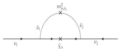
Figure 1: One-loop contribution to $m_{\nu}$ when $v_{\tilde{N}_{i}}=v_{\tilde{\nu}_{i}}=0$. Here $m^{2}_{\tilde{\nu}_{i}\tilde{\nu}_{j}}$ represents the sneutrino “Majorana” mass term which generates the neutrino mass involving the sneutrino-neutralino loop.

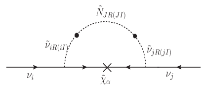
Figure 2: The same one-loop contribution to $m_{\nu}$ as in Fig.1 but represented in a different way. Here ${\tilde{N}}_{JR}$ and ${\tilde{N}}_{JI}$ are right handed sneutrino mass eigenstates which couple to ${\tilde{\nu}}_{i,j}$ to produce the one-loop effective neutrino mass term.

We begin by decomposing the sneutrino fields in terms of real and imaginary components. Thus one has

$$\tilde{\nu}_{i} = {\tilde{\nu}_{iR}+i\tilde{\nu}_{iI}\over\sqrt{2}},\hskip 8.5359pt\tilde{N}_{i}={\tilde{N}_{iR}+i\tilde{N}_{iI}\over\sqrt{2}},$$ (31)

where the components $\tilde{\nu}_{iR},\tilde{N}_{iR}$ are the $CP$-even and $\tilde{\nu}_{iI},\tilde{N}_{iI}$ are the $CP$-odd scalar fields. The mass terms of these scalars may be evaluated using the definition

$$M^{2}_{R,ij} = {\partial^{2}V\over\partial\Phi_{iR}\partial\Phi_{jR}},\ M^{2}_{p,ij}={\partial^{2}V\over\partial\Phi_{iI}\partial\Phi_{jI}},$$ (32)

where $\Phi$ represents a generic scalar field. Accordingly one obtains the following diagonal mass terms (assuming the right-chiral sneutrino states to be flavor diagonal) for the $CP$-even and $CP$-odd right-chiral sneutrinos:

$$M^{2}_{R,\tilde{N}_{i}\tilde{N}_{i}} = m^{2}_{\tilde{N}_{i}\tilde{N}_{i}^{\star}}+\lambda^{2}_{Ni}v_{s}^{2}$$

$$+ \hskip-7.11317pt(\lambda_{H}\lambda_{Ni}v_{d}v_{u}+\frac{1}{2}\lambda_{Ni}\lambda_{s}v_{s}^{2}+Am\lambda_{Ni}v_{s})$$

$$M^{2}_{P,\tilde{N}_{i}\tilde{N}_{i}} = m^{2}_{\tilde{N}_{i}\tilde{N}_{i}^{\star}}+\lambda_{Ni}^{2}v_{s}^{2}$$

$$- \hskip-7.11317pt(\lambda_{H}\lambda_{Ni}v_{d}v_{u}+\frac{1}{2}\lambda_{Ni}\lambda_{s}v_{s}^{2}+Am\lambda_{Ni}v_{s}).$$

Similarly, the interactions between $\tilde{N}_{iR,(iI)}$ and $\tilde{\nu}_{iR,(iI)}$ read as

$$C_{R,\tilde{\nu}_{i}\tilde{N}_{j}} = f^{\nu}_{ij}\lambda_{H}v_{d}v_{s}+f^{\nu}_{ij}\lambda_{Nj}v_{u}v_{s}+A^{\nu}f^{\nu}_{ij}v_{u},$$

$$C_{P,\tilde{\nu}_{i}\tilde{N}_{j}} = -f^{\nu}_{ij}\lambda_{H}v_{d}v_{s}+f^{\nu}_{ij}\lambda_{Nj}v_{u}v_{s}-A^{\nu}f^{\nu}_{ij}v_{u}.$$

The diagonal left-chiral sneutrino mass terms are shown in Eq.(LABEL:loopcoeff1). As we can see, the off-diagonal terms involving the left-chiral and right-chiral sneutrinos are much smaller compared to the diagonal terms since they are proportional to the small neutrino Yukawa couplings ($f^{\nu}\sim 10^{-6}$). Hence, we can compute the one-loop correction to the neutrino mass due to the small mixing of the right-chiral sneutrinos with the left-chiral sneutrinos. This is shown in Fig.2. Note that the right-chiral sneutrino mass matrix contains bilinear terms like $\lambda_{H}\lambda_{N_{i}}v_{d}v_{u}$, $\frac{\lambda_{s}\lambda_{N_{i}}v_{s}^{2}}{2}$ which are originated from the F-term contribution in the scalar potential. These are the new contributions to the right sneutrino masses in the present model and thus they are absent in seesaw models of MSSM with only right handed neutrino superfields. These terms will have important roles to play while calculating the one-loop correction to the neutrino mass matrix, even when the relevant soft breaking trilinear parameters are smaller. The loop contribution can be written as,

$$(m_{\nu})_{ij}^{loop} = {g_{2}^{2}\over 4}\sum_{\alpha}m_{{\widetilde{\chi}}_{\alpha}}(N_{\alpha 5}-\tan\theta_{w}N_{\alpha 4})^{2}[\sum_{J=1,2,3}C_{R_{iJ}}C_{R_{jJ}}I_{4}(m_{\tilde{\nu}_{iR}},m_{\tilde{\nu}_{jR}}m_{{\widetilde{\chi}}_{\alpha}},M_{\tilde{N}_{JR}})$$ (35)

$$- \sum_{J=1,2,3}C_{P_{iJ}}C_{P_{jJ}}I_{4}(m_{\tilde{\nu}_{iI}},m_{\tilde{\nu}_{jI}},m_{{\widetilde{\chi}}_{\alpha}},M_{\tilde{N}_{JI}})],$$

where the integral $I_{4}$ is given by,

$$I_{4}(m_{\tilde{\nu}_{iR}},m_{\tilde{\nu}_{jR}},m_{{\widetilde{\chi}}_{\alpha}},m_{X_{J}}) = \int{d^{4}q\over i(2\pi)^{4}}{1\over(q^{2}-m^{2}_{\tilde{\nu}_{iR}})(q^{2}-m^{2}_{\tilde{\nu}_{jR}})(q^{2}-m_{{\widetilde{\chi}}_{\alpha}}^{2})(q^{2}-m^{2}_{X_{J}})}.$$ (36)

Here $X_{J}$ denotes right chiral sneutrino states $\tilde{N}_{JR}$ or $\tilde{N}_{JI}$. One can always evaluate $I_{4}$ with the following analytical expressions,

$$I_{4}(m_{1},m_{2},m_{3},m_{4}) = {1\over m_{3}^{2}-m_{4}^{2}}[I_{3}(m_{1},m_{2},m_{4})-I_{3}(m_{1},m_{2},m_{3})],$$ (37)

$$I_{3}(m_{1},m_{2},m_{3}) = {1\over m_{2}^{2}-m_{3}^{2}}[I_{2}(m_{1},m_{2})-I_{2}(m_{1},m_{3})],$$ (38)

$$I_{2}(m_{1},m_{2}) = {1\over(4\pi)^{2}}{m_{2}^{2}\over m_{1}^{2}-m_{2}^{2}}\log{m_{1}^{2}\over m_{2}^{2}}.$$ (39)

Here, $m_{{\widetilde{\chi}}_{\alpha}}$ represents the eigenvalues of the NMSSM neutralino mass matrix. In the weak interaction basis $\left(\widetilde{S},{\widetilde{H}_{d}^{0}},{\widetilde{H}_{u}^{0}},\widetilde{B}^{0},\widetilde{W}^{0}\right)$, the mass matrix can be written as

$${\cal M} = \left(\begin{array}[]{ccccc}\lambda_{S}v_{s}&\lambda_{H}v_{u}&\lambda_{H}v_{d}&0&0\\ \lambda_{H}v_{u}&0&\lambda_{H}v_{s}&-g_{1}v_{d}/\sqrt{2}&g_{2}v_{d}/\sqrt{2}\\ \lambda_{H}v_{d}&\lambda_{H}v_{s}&0&g_{1}v_{u}/\sqrt{2}&-g_{2}v_{u}/\sqrt{2}\\ 0&-g_{1}v_{d}/\sqrt{2}&g_{1}v_{u}/\sqrt{2}&M_{1}&0\\ 0&g_{2}v_{d}/\sqrt{2}&-g_{2}v_{u}/\sqrt{2}&0&M_{2}\end{array}\right)\ .$$ (45)

The mixing matrix elements $N_{\alpha 5}$ and $N_{\alpha 4}$ are the wino and bino component of the neutralino ${\tilde{\chi}}_{\alpha}$. The expression (vide Eq.(35)) is the most general to compute the one-loop diagram (vide Fig.2). Nevertheless, we would consider a simplified scenario for illustration. In particular, we assume (i) identical values of $\lambda_{Ni}$ ( $\lambda_{Ni}\equiv\lambda_{N}$) for all three generations and (ii) soft-masses of the sneutrinos (both $\tilde{\nu}_{i}$ and $\tilde{N}_{i}$) are flavor blind. This results into identical mass values for all three $CP$-even right chiral sneutrinos ($M_{\tilde{N}_{RJ}}\equiv M_{\tilde{N}_{R}}$) and also for the three $CP$-odd states ($M_{\tilde{N}_{IJ}}\equiv M_{\tilde{N}_{I}}$). With these assumptions, it is possible to factor out the flavor structure from Eq.(35) and denote the remaining as the loop factor (LF) which is merely a constant. Then the loop contribution can be cast into a convenient form given by

$$(m_{\nu}^{\rm loop})_{ij}=(LF)\sum_{k=1}^{3}{{f^{\nu}_{iJ}}{f^{\nu}_{jJ}}},$$ (46)

where

$$LF = {g_{2}^{2}\over 4}\sum_{\alpha}m_{{\widetilde{\chi}}_{\alpha}}(N_{\alpha 5}-\tan\theta_{w}N_{\alpha 4})^{2}$$

$$\hskip-25.6073pt(I_{4}(m_{\tilde{\nu}},m_{\tilde{\nu}},m_{{\widetilde{\chi}}_{\alpha}},M_{\tilde{N}_{R}})C_{R}^{2}-I_{4}(m_{\tilde{\nu}},m_{\tilde{\nu}},m_{{\widetilde{\chi}}_{\alpha}},M_{\tilde{N}_{I}})C_{P}^{2}).$$

Here $C_{R}$ and $C_{P}$ represent the coefficients of $f^{\nu}_{ij}$ in Eq. (LABEL:mixing_sneu) and given as

$$C_{R} = \lambda_{H}v_{d}v_{s}+\lambda_{N}v_{u}v_{s}+A^{\nu}v_{u},$$ (48)

$$C_{P} = -\lambda_{H}v_{d}v_{s}+\lambda_{N}v_{u}v_{s}-A^{\nu}v_{u}.$$ (49)

Let us note that the coefficient $B_{Ri}$ can be written as

$$B_{Ri}=B_{N}M_{R}$$ (50)

where

$$B_{N} = \frac{1}{2}(\lambda_{H}v_{d}v_{u}/v_{s}+\frac{\lambda_{s}v_{s}}{2}+Am),$$

$$M_{R} = \lambda_{N}v_{s}.$$ (51)

Consequently the one-loop contribution can be cast into the well known formdavidson-king ; grossman-haber

$${m_{\nu}^{(loop)}}_{ij} = -{g_{2}^{2}{\Delta m_{{\tilde{\nu}}}}_{ij}\over 32\pi^{2}\cos^{2}\theta_{W}}\sum_{\alpha}\,f(y_{\alpha})|N_{\alpha k}|^{2}\,,$$ (52)

$$f(y_{\alpha}) = {\sqrt{y_{\alpha}}\left[y_{\alpha}-1-\ln(y_{\alpha})\right]\over(1-y_{\alpha})^{2}},$$

where $y_{\alpha}\equiv{m_{\tilde{\nu}}^{2}/m_{\tilde{\chi}^{0}_{\alpha}}^{2}}$ and $N_{\alpha k}\equiv N_{\alpha 5}\cos\theta_{W}-N_{\alpha 4}\sin\theta_{W}$ is the neutralino mixing matrix element and to order in $1/M^{3}_{R}$ the left sneutrino mass difference relative to the light neutrino mass is given by

$${{\Delta m_{\tilde{\nu}}}_{ij}\over{m_{\nu}}_{ij}} \simeq {{2(A_{\nu}+\mu\cot\beta-B_{N}-\frac{B_{N}(A_{\nu}+\mu\cot\beta)^{2}}{M^{2}_{R}})}\over m_{\tilde{\nu}}}.$$

Here we have used the relation $\Delta m^{2}_{\tilde{\nu}}=2m_{\tilde{\nu}}\Delta m_{\tilde{\nu}}$ and $m_{\tilde{\nu}}$ is an average left-sneutrino mass. In the present case all left handed sneutrino soft masses are assumed to be identical. The sneutrino Majorana mass $m^{2}_{{\tilde{\nu}}{\tilde{\nu}}}$ shown in Fig.1 is related to $\Delta m^{2}_{\tilde{\nu}}$ as $m^{2}_{{\tilde{\nu}}{\tilde{\nu}}}=\frac{1}{4}\Delta m^{2}_{\tilde{\nu}}$davidson-king . The quantity $\mu$ is defined as $\mu=\lambda_{H}v_{s}$.

In order to reproduce the result in Eq.(52), we assumed that $B_{N},m_{\tilde{N}\tilde{N}*}<M_{R}$ and $A_{\nu}>B_{N}$. Now, in addition if we assume $M_{R}>A_{\nu}$, the last term becomes negligible compared to the other terms in the expression Eq.(LABEL:sneutrino-mass-splitting) and this keeps only the terms to leading order in $1/M_{R}$. However, this is not always true as all soft SUSY breaking mass parameters as well as the right handed neutrino masses may have similar magnitudes as in the present scenario. Hence, rather than using Eq.(52), we evaluate the neutrino mass terms corrected up to one loop order, from

$$(m_{\nu}^{\rm total})_{ij}=(\frac{-v^{2}_{u}}{M_{R}}+LF)\sum_{k=1}^{3}{{f^{\nu}_{iJ}}{f^{\nu}_{jJ}}}.$$ (54)

Clearly, the coefficient of the loop contribution shifts the tree level neutrino masses by a constant amount. This coefficient involves the soft SUSY breaking parameters and in this work we explore the effect of these parameters on the neutrino mass matrix.

This simple structure of the neutrino mass matrix (vide Eq.(54)) can indeed be very helpful to examine the neutrino mixing pattern. In particular, we are interested to explore the conditions which could yield the mixing matrix into a tri-bimaximal structure. Thus we compare Eq.(54) with Eq.(15), where the latter provides with the neutrino mass matrix consistent with the tri-bimaximal mixing pattern. Then, with a symmetric neutrino Yukawa matrix, neutrino masses can be evaluated using the following expressions:

$$\frac{2}{3}m_{1}+\frac{1}{3}m_{2} = C[(f^{\nu}_{11})^{2}+(f^{\nu}_{12})^{2}+(f^{\nu}_{13})^{2}],$$

$$\frac{1}{6}(m_{1}+2m_{2}+3m_{3}) = C[(f^{\nu}_{12})^{2}+(f^{\nu}_{22})^{2}+(f^{\nu}_{23})^{2}],$$

$$= C[(f^{\nu}_{13})^{2}+(f^{\nu}_{23})^{2}+(f^{\nu}_{33})^{2}],$$

$$\frac{1}{3}(-m_{1}+m_{2}) = C[f^{\nu}_{11}f^{\nu}_{12}+f^{\nu}_{12}f^{\nu}_{22}+f^{\nu}_{13}f^{\nu}_{23}],$$

$$\frac{1}{3}(m_{1}-m_{2}) = C[f^{\nu}_{11}f^{\nu}_{13}+f^{\nu}_{12}f^{\nu}_{23}+f^{\nu}_{13}f^{\nu}_{33}],$$

$$\frac{1}{6}(-m_{1}-2m_{2}+3m_{3}) = C[f^{\nu}_{12}f^{\nu}_{13}+f^{\nu}_{22}f^{\nu}_{23}+f^{\nu}_{23}f^{\nu}_{33}].$$

Here the constant $C$ is defined as $(\frac{-v^{2}_{u}}{M_{R}}+LF)$. As a simple choice we consider, $f^{\nu}_{22}=f^{\nu}_{33}$ and also $f^{\nu}_{12}=f^{\nu}_{13}=0$ to obtain the solutions. This choice, coupled with the consistency condition $f^{\nu}_{11}=f^{\nu}_{22}-f^{\nu}_{23}$, leads to the following solutions of the neutrino spectra

$$m_{1} = m_{2}=(\frac{-v^{2}_{u}}{M_{R}}+LF)(f^{\nu}_{11})^{2},$$

$$m_{3} = (\frac{-v^{2}_{u}}{M_{R}}+LF)(2f^{\nu}_{22}-f^{\nu}_{11})^{2}.$$ (56)

It is obvious that the mass pattern as depicted above satisfies the desired tri-bimaximal structure of the neutrino mixing. The mass terms as expected, contain tree level contributions which are always negative. On the other hand, the loop contribution can go both ways depending on the sign of the soft SUSY breaking parameters. For a large $B_{R}$, which primarily depends on $Am$, the radiative correction to the neutrino masses could be enhanced to supersede the tree level resultsgrossman-haber .

Before presenting the numerical results a few comments regarding the lepton flavor violating (LFV) processes are in order. Recall that we assume flavor diagonal mass terms for the left and right chiral sneutrinos. The loop induced processes like $\mu\rightarrow e\gamma$, $\tau\rightarrow e\gamma$ or $\tau\rightarrow\mu\gamma$ can get contributions primarily via the couplings $B^{\nu}_{ij}$ or $B^{\prime\nu}_{ij}$ (see Eq.(LABEL:eq-eff-lagrangian) and (LABEL:loopcoeff1)). Clearly, any such contribution at the leading order would involve a product of two small neutrino Yukawa couplings $f^{\nu}_{ij}$ and are expected to be very suppressed. Moreover, our assumption $f^{\nu}_{12}=f^{\nu}_{13}=0$ would lead to vanishing contributions for the processes $\mu\rightarrow e\gamma$ and $\tau\rightarrow e\gamma$ in this model.

We now explore whether the obtained mass pattern could fit with the different hierarchical structure that we know so far. In particular, we show our numerical results to identify the regions in the parameter space consistent with the normal, inverted and quasi-degenerate neutrino mass pattern. In the numerical computation we choose different soft parameters and couplings in such a way, that the proper minima condition of the scalar potential is always satisfiedKitano-2001 .

The choices of various parameters are listed below. The value of $\tan\beta$ is taken to be equal to 10. In addition to that, other parameter choices are
(I) Superpotential parameters: $\lambda_{h}=-0.3$,   $\lambda_{s}=0.6$,   $\lambda_{N1}=\lambda_{N2}=\lambda_{N3}=\lambda_{N}=0.2$,
and
(II) Soft SUSY breaking parameters: $m_{S}$ = 100 GeV, $m_{{\tilde{N}}_{i}{\tilde{N}}_{i}^{*}}$ = 300 GeV, $m_{{\tilde{\nu}}_{i}}$ = 100 GeV, $A_{H}$ = 100 GeV, $A_{\nu}$ = 1000 GeV.

Apart from the above parameters which are fixed to the quoted values, we have also varied the parameter $Am$ in the calculation. This would cause changes in $v_{s}$ (vide Eq.(LABEL:vs_soln)), which in turn produces variation in the neutrino spectrum. We list the values of $Am$ and $v_{s}$ in table I.

$Am$ (GeV)	-600.0	-800.0	-1000.0	-1200.0
$v_{s}$ (GeV)	927.56	1280.76	1625.18	1965.67

Table 1: Different values of $v_{s}$ corresponding to the different values of the coupling parameter $Am$.

IV.2 Different Neutrino Spectra:

The two mass-squared differences shown in Eq.(1) indicate three possible neutrino mass hierarchieshierarchy , namely

1. Normal Hierarchy: this neutrino mass pattern can be established if $m_{1},m_{2}$ and $m_{3}$ are related with the observables $\sqrt{\Delta m^{2}_{21}}$ and $\sqrt{|\Delta m^{2}_{32}|}$ as

   $$m_{1}\approx m_{2}\sim\sqrt{\Delta m^{2}_{21}},\qquad m_{3}\sim\sqrt{|\Delta m^{2}_{32}|}.$$ (57)

   However, in principle $m_{1}$ can also be much smaller than $m_{2}$ or even be zero. Since in this case $m_{3}$ is much greater than both $m_{1}$ and $m_{2}$, we can approximately use the relation shown in Eq.(57) for illustration.

2. Inverted Hierarchy: this hierarchical scenario can be achieved if one chooses

   $$m_{1}\approx m_{2}\sim\sqrt{|\Delta m^{2}_{32}|},\qquad m_{3}\ll\sqrt{|\Delta m^{2}_{32}|}.$$ (58)

   We assume the maximum possible value for $m_{3}$ to be $\sim 0.01$ eV while the minimum value could be vanishing. Obviously, the solar mass squared difference $\Delta m^{2}_{21}$ will come from the small mass splitting between $m_{2}$ and $m_{1}$, where $\Delta m^{2}_{21}\ll m_{2},m_{1}$. Hence, for a simple minded analysis we can assume that $m_{2}=m_{1}$.

3. Degenerate Masses: finally this scenario is defined by

   $$m_{1}\approx m_{2}\approx m_{3}\gg\sqrt{|\Delta m^{2}_{32}|},$$ (59)

   Here we assume that the upper bound of the neutrino masses could be $0.33$ eV, which comes from the cosmological observations. The lower bound is chosen to be $0.1$ eV.

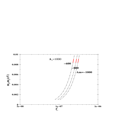
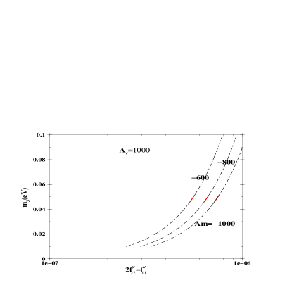
Figure 3: Normal hierarchy: variation of $m_{\nu}$ with the Yukawa parameters. The red (solid) segments denote the range of the Yukawa parameters that satisfy neutrino data. Each contour represents a separate set of $v_{s}$ and $Am$, as given in Table.1. All mass parameters are in GeV.

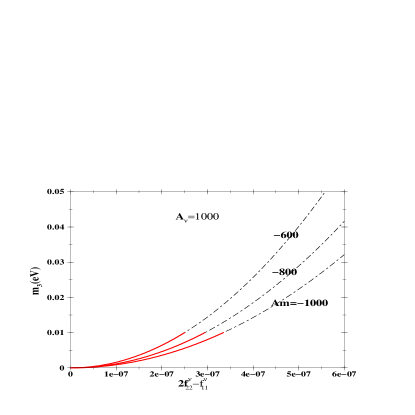
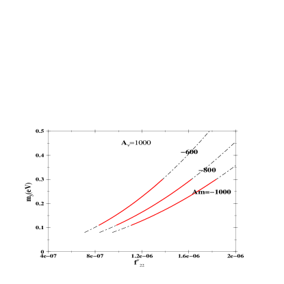
Figure 4: Variation of $m_{3}$ with the corresponding Yukawa parameter is shown for (a) inverted hierarchical mass pattern and also for (b) the degenerate spectrum. All mass parameters are in GeV.

In Fig3, three neutrino mass eigenvalues $m_{1},m_{2},m_{3}$, consistent with the normal hierarchical pattern, are plotted as functions of neutrino Yukawa couplings. The difference in the contours manifests how the neutrino masses depend on the soft bilinear coupling parameter ($Am$). The variation occurs, as $v_{s}$ depends on ($Am$), thereby acquiring a different value at the global minima which has already been mentioned in Table 1. In particular $|v_{s}|$ always increases as we increase $|Am|$ parameter which in turn increases the right handed neutrino masses. This results into a smaller value for $m^{tree}_{\nu}$. On the other hand, loop correction does not increase appreciably by this small variation of $Am$ if $A_{\nu}$ is around TeV scale as we will discuss later. We should note here that neutrino loop correction is always an order of magnitude smaller compared to the tree level value for the parameters we have chosen. Thus with increase in $Am$ parameter, one requires large values of Yukawa couplings to satisfy the neutrino data. The red zone in each contour (vide Fig3) represents the range of the Yukawa couplings that can satisfy the neutrino data.

In case of inverted hierarchy, we have shown the variation of $m_{3}$ with the respective Yukawa couplings in Fig.4. The other mass parameters $m_{1},m_{2}$ depend on the Yukawa coupling $f^{\nu}_{11}$, but that can be estimated from the Fig.3 if in that plot we replace $m_{3}$ in the y-axis by $m_{1}/m_{2}$ and $2f^{\nu}_{22}-f^{\nu}_{11}$ in the x-axis by $f^{\nu}_{11}$ (vide Eq.(56)). In fact knowing the value of the Yukawa coupling $f^{\nu}_{11}$ would allow us to determine the coupling $f^{\nu}_{22}$.

The Fig.4 depicts the variation of $m_{3}$ with the Yukawa coupling $f^{\nu}_{22}$ for quasi-degenerate mass scenario. In this scenario, the neutrino spectrum is approximately degenerate i.e., $m_{1}$, $m_{2}$ and $m_{3}$ turn out to be almost identical if one chooses $f^{\nu}_{23}$ much smaller compared to the diagonal Yukawa coupling $f^{\nu}_{22}$, which essentially means that $f^{\nu}_{22}\approx f^{\nu}_{11}$.

Finally a few comments on the dependence of the one-loop contribution to the neutrino mass on the soft SUSY breaking parameters $Am$ and $A_{\nu}$. The loop contribution is always suppressed unless the parameter $A_{\nu}$ is sufficiently large as can be seen from Fig.5. As for illustration, the Yukawa couplings are chosen as $f^{\nu}_{11}=1.75\times 10^{-7}$ and $f^{\nu}_{22}=f^{\nu}_{33}=3.95\times 10^{-7}$. Similarly, we choose $M_{1}$ = 60 GeV and $M_{2}$ = 120 GeV, where $M_{1}$ and $M_{2}$ are the $U(1)$ and $SU(2)$ gaugino mass parameters, respectively. For larger values of electroweak gaugino masses, the one-loop contribution would be reduced further. For $Am$ = -1 TeV, higher $A_{\nu}$ values $\sim$ 13 TeV can satisfy the current neutrino data. However, even if $A_{\nu}$ is $\sim$ 13 TeV, the quantity $A_{\nu}f^{\nu}$ is very small, i.e., $\sim 10^{-2}$ GeV. Note that for such a choice of the parameter space, the tree level values of the neutrino masses are not sufficient to accommodate the three flavor global neutrino data. Increasing the value of $Am$ requires relatively smaller value of $A_{\nu}$ ($\sim$ 7 TeV) to reproduce the neutrino data. It is very important to point out that, for a fixed $\lambda_{s}$ and $\lambda_{Ni}$ one cannot increase the trilinear coupling parameter $Am$ to an arbitrary high value as the right-chiral sneutrinos may turn out to be tachyonic. Thus, a relatively larger soft trilinear parameter $A_{\nu}$ is required to enhance the one-loop contribution to neutrino masses.

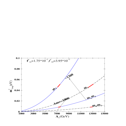
Figure 5: Variation of the $m^{loop}_{\nu}$ with $A^{\nu}$ in the normal hierarchical scenario. All mass parameters are in GeV.

The requirement of a large $A_{\nu}$ can be understood from the following discussion.

• The one-loop contribution to the neutrino mass originating from the mass splitting in the left-handed sneutrinos depends on the parameters $\mu$, $A_{\nu}$ and $B_{N}$ as can be seen from Eqs.(52) and (LABEL:sneutrino-mass-splitting). It has been argued in Ref.grossman-haber , that in order to have the one-loop contribution to the neutrino mass comparable to its tree level value, the ratio $\Delta m_{{\tilde{\nu}}_{ij}}/m_{\nu}$ should be $\sim 10^{3}$.

• Substituting $\mu=\lambda_{H}v_{s}$ and the expression for $B_{N}$ from Eq.(IV.1), we may write ${\Delta m_{\tilde{\nu}}}_{ij}/m_{\nu}\simeq 2(A_{\nu}+\lambda_{H}v_{s}\cot\beta-(\frac{1}{4}\lambda_{s}v_{s}+Am/2+\lambda_{H}v_{d}v_{u}/2v_{s})(1+(A_{\nu}+\lambda_{H}v_{s}\cot\beta)^{2})/M^{2}_{R})/m_{\tilde{\nu}}$. We can see from the above expression that one may increase either $Am$ or $A^{\nu}$ parameter to enhance the one-loop contribution to make it countable. But in the present context, raising the soft parameter $Am$ alone would not serve the purpose. This is because the VEV $v_{s}$ increases significantly with $|Am|$ (vide Table. 1). Thus there is always a partial cancellation between different terms in the above expression for the left sneutrino mass splitting. In particular, the effective bilinear coupling $B_{N}$ is reduced because of this partial cancellation. In addition, we choose the sign of the coupling $\lambda_{H}$ as negative in order to determine the correct global minima. This also causes a partial cancellation between various terms, but to a lesser extent. Considering this cancellation effect in mind, it is easy to check that the ratio ${\Delta m_{\tilde{\nu}}}_{ij}/m_{\nu}$ always reside near the value $\sim 10$ with the soft parameters $A^{\nu}$ and $B_{N}$ around the TeV scale.

• Now, as mentioned above, the trilinear coupling parameter $Am$ is restricted if one does not want the right chiral sneutrinos to become tachyonic. Of course this depends on the choice of the soft “Dirac” mass term $m_{{\tilde{N}}{\tilde{N}}^{*}}$ of the $\tilde{N}$s, which we have chosen to have a quite moderate value (300 GeV) in this case. However, the parameter $A^{\nu}$ can be pushed to a reasonably high value without affecting any other results. This explains why a large $A^{\nu}$ parameter is required to make the one-loop contribution to the neutrino mass comparable to its tree level value.

V Signatures at LHC

It is extremely important to investigate the possible signatures of this TeV scale seesaw mechanism at the LHC. One of the search strategies could be to produce the right-handed neutrino $N$ (or the corresponding right-handed sneutrino ${\tilde{N}}$) with a large enough cross-section and then look at the decay branching ratios in different available modes. However, in this type of models the production of TeV scale right-handed neutrinos (or sneutrinos) at the LHC is suppressed by the light neutrino mass neutrino_mass_LHC_review . Nevertheless, it is possible to construct models where the production mechanism of the right-handed neutrino (sneutrino) can be decoupled from the neutrino mass generation. For example, extended gauge symmetries such as $U(1)_{B-L}$ or $SU(2)_{R}$ may offer extra gauge bosons near the TeV scale whose couplings to quarks and the right-handed neutrino (sneutrino) are unsuppressed mohapatra-marshak . In such models a single or a pair of right-handed neutrinos can be produced with large cross sections leading to dilepton signals (same-sign) with no missing energy (see the first reference of other-early-seesaw and keung-senjanovic ; dittmar-etal ; ferrari-etal ; gninenko-etal ), trilepton signals del-aguila-etal or four-lepton signals valle-4lepton ; del-aguila-etal-2 ; santosh-katri-shaaban-okada-prl .

In the context of the present model the left-sneutrino “Majorana” mass term can lead to oscillation between the left-chiral sneutrino and the corresponding anti-sneutrino hirsch-klapdor-kovalenko ; grossman-haber ; dedes-haber-rosiek . This can be interpreted as the observation of a sneutrino decaying into a final-state with a “wrong-sign” charged lepton. In order to have a large oscillation probability the total decay width $\Gamma$ of the sneutrino/antisneutrino and the mass splitting $\Delta m$ must be of the same order. Since $\Delta m$ is constrained by the neutrino data, one needs a very small total decay width of the sneutrino/antisneutrino. It has been shown in grossman-haber that this can be achieved in a scenario where the lighter stau is long-lived and the left-chiral sneutrino can only have 3-body decay modes involving the lighter stau in the final states. This can lead to signals such as like-sign dileptons, single charged lepton plus like-sign di-staus (leading to heavily ionizing charged tracks) or like-sign di-stau charged tracks at future linear colliders grossman-haber ; choietal ; honkavaara-huitu-roy or at the LHC honkavaara1 . The resulting charge asymmetry of the final states can be measured to get an estimate of the sneutrino-antisneutrino oscillation probability honkavaara1 . In addition, for a very small sneutrino decay width one can also observe a displaced vertex in the detector. However, a detailed study of such signals in the context of the present model is beyond the scope of the present paper.

In comparison, now we discuss briefly the signatures of R-parity violating models in general. In models with spontaneous violation of R-parity, the singlet sneutrino vacuum expectation value leads to the existence of a Majoron which is an additional source of missing energy. This can change the decay pattern of the lightest Higgs and the lightest neutralino with the corresponding signatures at the LHC. For more details and the relevant references the reader is referred to Ref.neutrino_mass_LHC_review . In the case of bilinear R-parity violation, the ratios of certain decay branching ratios of the LSP show very nice correlation with the neutrino mixing angles. This can lead to very interesting signatures at the LHC where comparable numbers of events with muons and taus, respectively, can be observed in the final state Roy-Mukhopadhyaya-Vissani ; choi-chun-kang-lee ; romao-diaz-hirsch-porod-valle ; datta-mukhopadhyaya-vissani ; porod-hirsch-romao-valle ; chun-jung-kang-park ; jung-kang-park-chun .

From the above discussion we see that the canonical type-I supersymmetric seesaw case that we have considered in this paper has characteristic signatures which can be tested at the LHC. At the same time one can also distinguish the predictions of this model with those of the models with spontaneous or bilinear R-parity violating scenarios.

VI Conclusions

We have studied the neutrino masses and mixing in an R-parity conserving supersymmetric standard model with three right handed neutrino superfields ${\hat{N}}_{i}$ and another gauge singlet superfield ${\hat{S}}$. This model is similar to the next-to-minimal supersymmetric standard model (NMSSM), where the scalar component of ${\hat{S}}$ gets a VEV to generate a $\mu$-term of correct order of magnitude. In addition, the same VEV also generates TeV scale Majorana masses for the right handed neutrinos. The small neutrino masses are generated at the tree level by the usual seesaw mechanism at the TeV scale. We also calculate the one-loop contribution to the neutrino mass matrix and investigate the constraints on the model parameters to produce the tri-bimaximal pattern of neutrino mixing for three different neutrino mass hierarchies. Neutrino mass matrix gets contribution at the one-loop level controlled by the sneutrino “Majorana” mass terms. We show that the one-loop contribution can be important for certain choices of the soft SUSY breaking parameters. This we have demonstrated by evaluating the one-loop contribution in two different ways. In particular, we observe that the one-loop contributions can be significant when the soft SUSY breaking trilinear parameter $A_{\nu}f^{\nu}$ is $\sim{\cal O}(10^{-3}$ GeV) with $A_{\nu}\sim$ 10 TeV. This observation is quite robust and does not change much if one introduces a small $\theta_{13}$ in the neutrino sector. Our choice of neutrino Yukawa couplings also predict vanishing contributions to the lepton flavor violating processes $\mu\rightarrow e\gamma$ and $\tau\rightarrow e\gamma$ as well as an extremely suppressed contribution to $\tau\rightarrow\mu\gamma$.

As has been stated earlier, it is also possible to have non-zero vacuum expectation values for the left and right chiral sneutrinos. In that case, R-parity is violated spontaneously. The neutrino mass matrix can have contributions from two different sources, namely, the effective bilinear R-parity violating interactions and the TeV-scale seesaw mechanism. One-loop contributions to the neutrino mass matrix can be very important in this case too. However, the tree level and one-loop calculations are rather involved and require a separate discussion altogether. We plan to present these results in a subsequent paperdebottam-future .

The characteristic signatures of this model at the LHC include like-sign dilepton (without missing energy), trilepton or four lepton final states as well as single lepton plus two heavily ionizing charged tracks or only two heavily ionizing charged tracks stemming from long-lived staus. By looking at these signals one can possibly distinguish this model from the models of spontaneous or bilinear R-parity violation.

Acknowledgments
DD thanks P2I, CNRS for the support received as a post-doctoral fellow. We thank Pradipta Ghosh, Biswarup Mukhopadhyaya and Subhendu Rakshit for fruitful discussions. DD would also like to thank Asmaa Abada and Gregory Moreau for some valuable comments and suggestions. He is also thankful to the Department of Theoretical Physics, Indian Association for the Cultivation of Science (IACS), where a part of this work has been done.

References

- (1) For early references, see, P. Fayet, Nucl. Phys. B90, 104 (1975); Phys. Lett. B69, 489 (1977); G. R. Farrar and P. Fayet, Phys. Lett. B76, 575 (1978); C. S. Aulakh and R. N. Mohapatra, Phys. Lett. B119, 136 (1982); L. J. Hall and M. Suzuki, Nucl. Phys. B231, 419 (1984); I. H. Lee, Phys. Lett. B138, 121 (1984); I. H. Lee, Nucl. Phys. B246, 120 (1984); G. G. Ross and J. W. F. Valle, Phys. Lett. B151, 375 (1985); J. R. Ellis, G. Gelmini, C. Jarlskog, G. G. Ross and J. W. F. Valle, Phys. Lett. B150, 142 (1985); A. Masiero and J.W.F. Valle, Phys. Lett. B251, 273 (1990).
- (2) For reviews on R-parity violation, see, e.g., R. Barbier et al., Phys. Rep. 420, 1 (2005); M. Chemtob, Prog. Part. Nucl. Phys. 54, 71 (2005).
- (3) J.C. Romao, C.A. Santos, J.W.F. Valle, Phys. Lett. B288, 311 (1992).
- (4) G.F. Giudice, A. Masiero, M. Pietroni, A. Riotto, Nucl. Phys. B396, 243 (1993) [arXiv:hep-ph/9209296].
- (5) I. Umemura and K. Yamamoto, Nucl. Phys. B423, 405 (1994).
- (6) M.C. Gonzalez-Garcia, J.C. Romao, J.W.F. Valle, Nucl. Phys. B391, 100 (1993).
-
(7)
R. Adhikari and B. Mukhopadhyaya,
Phys. Lett. B378, 342 (1996) [arXiv:hep-ph/9601382];
Erratum-ibid. B384, 492 (1996). - (8) M. Hirsch, A. Vicente, W. Porod, Phys. Rev. D77, 075005 (2008) [arXiv:0802.2896].
- (9) B. Mukhopadhyaya, S. Roy and F. Vissani, Phys. Lett. B443, 191 (1998) [hep-ph/9808265].
- (10) S.Y. Choi, E. J. Chun, S. K. Kang, J. S. Lee, Phys. Rev. D60, 075002 (1999) [hep-ph/9903465].
- (11) J.C. Romao, M.A. Diaz, M. Hirsch, W. Porod, J.W.F Valle, Phys. Rev. D61, 071703 (2000) (Rapid Communications) [hep-ph/9907499].
- (12) A. Datta, B. Mukhopadhyaya and F. Vissani, Phys. Lett. B492, 324 (2000) [hep-ph/9910296].
- (13) W. Porod, M. Hirsch, J. Romao and J.W.F. Valle, Phys. Rev. D63, 115004 (2001) [hep-ph/0011248].
- (14) E. J. Chun, D-W. Jung, S. K. Kang, J. D. Park, Phys. Rev. D66, 073003 (2002) [hep-ph/0206030].
- (15) D-W. Jung, S. K. Kang, J. D. Park, E. J. Chun, JHEP08, 017 (2004) [arXiv:hep-ph/0407106].
- (16) P. Minkowski, Phys. Lett. B 67, 421 (1977); M. Gell-Mann, P. Ramond and R. Slansky, Published in Supergravity, P. van Nieuwenhuizen D.Z. Freedman (eds.), North Holland Publ. Co., 1979. Published in Stony Brook Wkshp.1979:0315 (QC178:S8:1979); T. Yanagida, in Proceedings of the Workshop on the Unified Theory and the Baryon Number in the Universe (O. Sawada and A. Sugamoto, eds.), KEK, Tsukuba, Japan, 1979, p. 95; S. L. Glashow, Proceedings of the 1979 Cargèse Summer Institute on Quarks and Leptons (M. Lévy, J.-L. Basdevant, D. Speiser, J. Weyers, R. Gastmans, and M. Jacob, eds.), Plenum Press, New York, 1980, pp. 687–713; R. N. Mohapatra and G. Senjanovic, Phys. Rev. Lett. 44, 912 (1980).
- (17) J. Schechter and J.W.F. Valle, Phys. Rev. D22, 2227 (1980); Phys. Rev. D25, 774 (1982); T.P. Cheng and L.-F. Li, Phys. Rev. D22, 2860 (1980).
- (18) Y. Grossman and H. E. Haber, Phys. Rev. Lett. 78, 3438 (1997) [arXiv:hep-ph/9702421].
- (19) S. F. King, Phys. Lett. B 439, 350 (1998) [arXiv:hep-ph/9806440].
- (20) S. Davidson and S. F. King, Phys. Lett. B 445, 191 (1998) [arXiv:hep-ph/9808296].
- (21) M. Maniatis, arXiv:0906.0777 [hep-ph]; U. Ellwanger, C. Hugonie and A. M. Teixeira, arXiv:0910.1785 [hep-ph].
- (22) P.N. Pandita, Phys. Lett. B 318, 338 (1993); P.N. Pandita, Z. Phys. C 59, 575 (1993); U. Ellwanger et al., Z. Phys. C 67, 665 (1995); U. Ellwanger et al., Nucl. Phys. B 492, 21 (1997); U. Ellwanger and C. Hugonie, Eur. Phys. J. C 13, 681 (2000); A. Dedes et al., Phys. Rev. D 63, 055009 (2001); U. Ellwanger et al., arXiv:hep-ph/0111179; D. G. Cerdeno et al., JHEP 0412, 048 (2004); U. Ellwanger et al., JHEP 0507, 041 (2005); U. Ellwanger and C. Hugonie, Phys. Lett. B 623, 93 (2005); G. Bélanger et al., JCAP 0509, 001 (2005); A. Djouadi et al., JHEP 0807, 002 (2008); A. Djouadi, U. Ellwanger and A. M. Teixeira, JHEP 0904, 031 (2009).
- (23) P.N. Pandita and P.F. Paulraj, Phys. Lett. B462, 294 (1999); P.N. Pandita, Phys. Rev. D64, 056002 (2001); M. Chemtob and P.N. Pandita, Phys. Rev. D 73, 055012 (2006); A. Abada and G. Moreau, J. High Energy Phys., 08, 044 (2006).
- (24) A. Abada, G. Bhattacharyya, and G. Moreau, Phys. Lett. B642, 503 (2006).
- (25) R. Kitano and K. y. Oda, Phys. Rev. D 61, 113001 (2000) [arXiv:hep-ph/9911327].
- (26) P. Fayet, Nucl. Phys. B90, 104 (1975); R. Barbieri, S. Ferrara, and C.A. Savoy, Phys. Lett. 119B, 343 (1982); J. Ellis, J.F. Gunion, H.E. Haber, L. Roszkowski, and F. Zwirner, Phys. Rev. D39, 844 (1989).
- (27) E. K. Akhmedov, arXiv:hep-ph/0001264; A. Strumia and F. Vissani, Nucl. Phys. B726, 294 (2005); R. N. Mohapatra and A. Y. Smirnov, hep-ph/0603118.
- (28) E. Komatsu et al. [WMAP Collaboration], Five-Year Wilkinson Microwave Anisotropy Probe (WMAP) Observations:Cosmological Interpretation, Astrophys. J. Suppl. 180, 330 (2009) [arXiv:0803.0547 [astro-ph]].
- (29) H. V. Klapdor-Kleingrothaus, I. V. Krivosheina, A. Dietz and O. Chkvorets, Phys. Lett. B 586, 198 (2004) [arXiv:hep-ph/0404088]; H. V. Klapdor-Kleingrothaus and I. V. Krivosheina, Mod. Phys. Lett. A 21, 1547 (2006); C. Arnaboldi et al. [CUORICINO Collaboration], Phys. Rev. C 78, 035502 (2008) [arXiv:0802.3439 [hep-ex]].
- (30) T. Schwetz, M. A. Tortola and J. W. F. Valle, New J. Phys. 10, 113011 (2008) [arXiv:0808.2016 [hep-ph]].
- (31) P.F. Harrison, D.H. Perkins and W.G. Scott, Phys. Lett. B 530, 167 (2002).
- (32) D. G. Cerdeno, C. Munoz and O. Seto, Phys. Rev. D 79, 023510 (2009) [arXiv:0807.3029 [hep-ph]]; D. G. Cerdeno and O. Seto, JCAP 0908, 032 (2009) [arXiv:0903.4677 [hep-ph]].
- (33) M. Frank, K. Huitu, and T. Rüppell, Eur. Phys. J. C52, 413 (2007).
- (34) M. Mitra, arXiv:0912.5291 [hep-ph].
- (35) C. C. Jean-Louis and G. Moreau, arXiv:0911.3640 [hep-ph].
- (36) D. E. López-Fogliani and C. Muñoz, Phys. Rev. Lett 97, 041801 (2006); N. Escudero, D.E. López-Fogliani, C. Muñoz, and R.R. de Austri, J. High Energy Phys. 12, 099 (2008); J. Fidalgo, D.E. López-Fogliani, C. Muñoz, and R. Ruiz de Austri, J. High Energy Phys. 08, 105 (2009) [arXiv:0904.3112].
- (37) P. Ghosh and S. Roy, J. High Energy Phys. 04, 069 (2009).
- (38) P. Ghosh, P. Dey, B. Mukhopadhyaya and S. Roy, J. High Energy Phys. 05, 087 (2010) arXiv:1002.2705 [hep-ph].
- (39) A. Bartl, M. Hirsch, S. Liebler, W. Porod, and A. Vicente, J. High Energy Phys. 05, 120 (2009) [arXiv:0903.3596].
- (40) B. Mukhopadhyaya and R. Srikanth, Phys. Rev. D 74, 075001 (2006) [arXiv:hep-ph/0605109].
- (41) N. Arkani-Hamed, L. J. Hall, H. Murayama, D. Tucker-Smith and N. Weiner, Phys. Rev. D 64, 115011 (2001) [arXiv:hep-ph/0006312]; N. Arkani-Hamed, L. J. Hall, H. Murayama, D. Tucker-Smith and N. Weiner, arXiv:hep-ph/0007001; F. Borzumati and Y. Nomura, Phys. Rev. D 64, 053005 (2001) [arXiv:hep-ph/0007018]; J. March-Russell and S. M. West, Phys. Lett. B 593, 181 (2004) [arXiv:hep-ph/0403067]; B. Mukhopadhyaya, P. Roy and R. Srikanth, Phys. Rev. D 73, 035003 (2006); J. March-Russell, C. McCabe, M. McCullough, JHEP1003, 108 (2010) arXiv:0911.4489 [hep-ph].
- (42) D. Das and S. Roy, in preparation.
- (43) Y. Grossman and H. E. Haber, Phys. Rev. D 67, 036002 (2003) [arXiv:hep-ph/0210273].
- (44) E. Ma, Phys. Rev. D 66, 117301 (2002); A. Joshipura, Proc. Indian Natl. Sci. Acad A 70, 223 (2004).
- (45) A. Atre, T. Han, S. Pascoli and B. Zhang, J. High Energy Phys. 05, 030 (2009) arXiv:0901.3589 [hep-ph].
- (46) P. Nath et al., Nucl. Phys. Proc. Suppl. 200–202, 185–417 (2010) arXiv:1001.2693 [hep-ph].
- (47) R.N. Mohapatra and R.E. Marshak, Phys. Rev. Lett. 44, 1316 (1980).
- (48) W.-Y. Keung and G. Senjanovic, Phys. Rev. Lett. 50, 1427 (1983).
- (49) M. Dittmar et al., Nucl. Phys. B332, 1 (1990).
- (50) A. Ferrari et al., Phys. Rev. D62, 013001 (2000).
- (51) S.N. Gninenko, M.M. Kirsanov, N.V. Krasnikov, and V.A. Matveev, Phys. Atom. Nucl. 70, 441 (2007).
- (52) F. del Aguila, J.A. Aguilar-Saavedra, and J. de Blas, arXiv:0910.2720.
- (53) J.W.F. Valle, Phys. Lett. B196, 157 (1987).
- (54) F. del Aguila and J.A. Aguilar-Saavedra, J. High Energy Phys. 11, 072 (2007).
- (55) For a more recent reference, see e.g., K. Huitu, S. Khalil, H. Okada, and S.K. Rai, Phys. Rev. Lett. 101, 181802 (2008).
- (56) M. Hirsch, H.V. Klapdor-Kleingrothaus, and S.G. Kovalenko, Phys. Lett. B398, 311 (1997).
- (57) A. Dedes, H.E. Haber, and J. Rosiek, J. High Energy Phys. 11, 059 (2007).
- (58) K. Choi, K. Hwang, and W.Y. Song, Phys. Rev. Lett. 88, 141801 (2002).
- (59) T. Honkavaara, K. Huitu, and S. Roy, Phys. Rev. D73, 055011 (2006).
- (60) D.K. Ghosh, T. Honkavaara, K. Huitu, S. Roy, Phys. Rev. D79, 055005 (2009); arXiv:1005.1802.