Vibrational wave packet induced oscillations in two-dimensional electronic spectra.
II. Theory

Abstract

We present a theory of vibrational modulation of two-dimensional coherent Fourier transformed electronic spectra. Based on an expansion of the system’s energy gap correlation function in terms of Huang-Rhys factors, we explain the time-dependent oscillatory behavior of the absorptive and dispersive parts of two-dimensional spectra of a two-level electronic system, weakly coupled to intramolecular vibrational modes. The theory predicts oscillations in the relative amplitudes of the rephasing and non-rephasing parts of the two-dimensional spectra, and enables to analyze time dependent two-dimensional spectra in terms of simple elementary components whose line-shapes are dictated by the interaction of the system with the solvent only. The theory is applicable to both low and high energy (with respect to solvent induced line broadening) vibrations. The results of this paper enable to qualitatively explain experimental observations on low energy vibrations presented in the preceding paper [A. Nemeth et al, arXiv:1003.4174v1] and to predict the time evolution of two-dimensional spectra in ultrafast ultrabroad band experiments on systems with high energy vibrations.

I Introduction

Multi-dimensional ultrafast spectroscopic techniques open an increasingly broad experimental window into the dynamics of molecular systems on femtosecond and picosecond time scales. Important experimental insights have been obtained by studying dynamics of small systems such as vibrations of small molecules, peptides and proteins HochstrasserReview09 , hydrogen bonding networks in water Fecko06a and peptides Hamm06 , and electronic transitions in dye molecules Brixner04b ; Nemeth08a . At the same time, multi-dimensional spectroscopy have proven its strength on complex systems ranging from conjugated polymers Scholes09a ; Scholes09b , nanotubes Nemeth09b , protein chromophore complexes Brixner05a ; Zigmantas06a ; Engel07a ; Lee07 , all the way to solid state systems Nelson09 . The experimental work has been closely interlinked with theoretical efforts JonasReview ; Cho05a ; Mancal06a ; Pisliakov06a ; Cho08a ; Cho05b ; Brugemann06 ; Brugemann07 ; Abramavicius09a ; Abramavicius08a ; YCC07a ; YCC08a ; Egorova07 ; Egorova08 which provided interpretation to this rich source of experimental information. One of the most interesting recent topics in this field was stimulated by the observation of oscillatory modulations of two-dimensional (2D) spectra, that were assigned to the presence and time-evolution of electronic wavepackets Engel07a ; Scholes99a ; Pisliakov06a . While the oscillatory effects were predicted theoretically from exciton theory Pisliakov06a ; Brugemann06 , the details of the observed processes suggest that theories traditionally applied to model energy relaxation and transfer in these systems underestimate the role of coherence effects. For example, the decoupling of exciton population and coherence dynamics (secular approximation) seems not to be a valid approximation for the photosynthetic protein FMO Engel07a .

Favorable properties of the studied multichromophoric systems, together with a partial success of exciton theory allowed to exclude vibrational coherence as a source of the oscillatory effects in the experiments on FMO Engel07a . In general however, a complementary understanding of the time-dependent spectral features of vibrational origin are clearly required in order to be able to disentangle the two effects. To this end, the topic of this and the preceding experimental paper, Ref. Nemeth09a (paper I), is a system which can exhibit only vibrational coherence, a two-level electronic system interacting with well-defined intramolecular vibrational modes.

For the description of non-linear spectroscopic signals of simple few electronic level systems with negligible relaxation between the levels, the non-linear response functions derived in the second order cumulant approximation (see e.g. MukamelBook ) provide a framework of unprecedented utility. The non-linear optical response of such a system can be expressed in terms of line-broadening functions, which are related to the electronic energy gap correlation function MukamelBook . Few electronic level systems provide models which enable to disentangle the content of experimental data otherwise difficult to interpret. For example, three pulse photon echo peakshift was identified by Cho et al. Cho96 to reveal the energy gap correlation function. Two-color photon echo peakshift has been found to measure excitonic coupling in a dimer Yang99 or differences between energy gap correlation functions of two chromophores Mancal04a . Basic 2D spectral line-shapes were classified by Tokmakoff Tokmakoff2000 based on a two-level system, and finally, the relation between the non-linear spectroscopic signals and the normalized energy gap correlation function was studied by de Boeij et al. deBoeij96 and for 2D spectra by Lazonder et al. Pshenichnikov06 , to name but a few examples.

In some of these works, insightful information was obtained by expanding the line-shape functions (or energy gap correlation functions) in terms of a suitable parameter, e.g. the time delay between two interactions. In the present study, we follow the same general approach and expand the line-shape correlation functions (describing the interaction of an electronic transition with an intra-molecular vibrational mode) in terms of another suitable parameter, the Huang-Rhys factor $\lambda/\omega$. Here, $\lambda$ is the reorganization energy and $\omega$ the frequency of the mode. The applicability of a low order expansion of the response functions in terms of the Huang-Rhys factor to the description of the 2D experiment is obviously system-dependent but for the dye molecule studied in Refs. Nemeth09a and Nemeth08a the qualitative results of the theory presented in this paper were confirmed by a full response function simulation of the 2D spectrum Nemeth08a .

One of the first theoretical analyses of the vibrational line-shapes in electronic 2D spectra was done by Egorova et al. Egorova07 ; Egorova08 using the density matrix propagation method. We complement this work by performing a detailed analysis of a two-level electronic system within the response function theory, where vibrational levels are not considered explicitely. Unlike in Refs. Egorova07 and Egorova08 we consider both rephasing and non-rephasing parts of the 2D spectrum, and we study time dependent modulations of the 2D spectrum by slow vibrational modes.

This paper is organized as follows. In the next section, we shortly review two-dimensional Fourier transformed spectroscopy and its theoretical description. In Section III we introduce the non-linear response functions and the line-shape functions which form the basis of our description of the 2D spectra. In Section IV we decompose the total 2D line-shape into several components according to their time dependence and derive elementary 2D line-shapes, which can be used to construct the total 2D spectrum. The time evolution of 2D spectra modulated by low and high energy modes are analyzed in Section V. Our conclusions are summarized in Section VI.

II Two-Dimensional Fourier Transformed Spectroscopy

The principles of Two-Dimensional Fourier Transformed Spectroscopy (2D-FT) where described in detail in many references (see e.g. Brixner04b ; JonasReview ) including the preceding paper, Ref. Nemeth09a . Here, we sum up results important for the theoretical modeling of the 2D-FT spectra in this paper.

In 2D-FT we use three laser pulses with wave-vectors ${\bf k}_{1}$, ${\bf k}_{2}$, and ${\bf k}_{3}$ arriving at the sample at times $\tau_{1}$, $\tau_{2}$, and $\tau_{3}$, respectively. In case of sufficiently weak excitation pulses, the intensity of the signal observed in the direction of $-{\bf k}_{1}+{\bf k}_{2}+{\bf k}_{3}$ is of third order in the total intensity of the incident light and the signal can be well described by third order time-dependent perturbation theory. The propagation of light through a material sample is influenced by the light-induced polarization, which is proportional to a material response function. The total third order response of the system to an excitation by three successive interactions with an external electric field of a laser is

$${\cal R}^{(3)}(t_{3},t_{2},t_{1})=\Theta(t_{3})\Theta(t_{2})\Theta(t_{1})$$

$$\times\left(\frac{i}{\hbar}\right)^{3}\sum_{n=1}^{4}\left\{R_{n}(t_{3},t_{2},t_{1})-R_{n}^{*}(t_{3},t_{2},t_{1})\right\},$$ (1)

where $\Theta(t)$ is the Heaviside step-function. The $R_{n}$ functions are defined according to the standard notation of Ref. MukamelBook , and represent different perturbative contributions (know as Liouville pathways) to the total response. The response is a function of three time variables, where $t_{1}$ denotes the delay between the first and second interaction, $t_{2}$ denotes the delay between the second and third interaction, and $t_{3}$ is the delay between the last interaction and the measurement. The polarization of the sample at time $t_{3}$ after the arrival of the third pulse is given by a three-fold convolution of the response function, Eq. (1), with the incoming electric fields. For very short pulses (impulsive limit) one can identify times $t_{1}$ and $t_{2}$ with the delays between the pulses ($t_{1}=|\tau_{2}-\tau_{1}|$, $t_{2}=|\tau_{3}-\tau_{2}|$) and one can approximate the polarization by those parts of the above expression that survive the so-called rotating wave approximation (RWA) (see e.g. Ref. Brixner04b ). This yields $P_{s}^{(3)}(t_{3},t_{2},t_{1})\approx{\cal R}_{rwa}^{(3)}(t_{3},t_{2},t_{1})$. With different ordering of the pulses ${\bf k}_{1}$ and ${\bf k}_{2}$, ${\cal R}_{rwa}^{(3)}$ contains different Liouville pathways. In particular

$$P_{s}^{(3)}(t_{3},t_{2},t_{1})\approx-iR_{2}(t_{3},t_{2},t_{1})-iR_{3}(t_{3},t_{2},t_{1}),$$ (2)

for $\tau_{1}<\tau_{2}$ and

$$P_{s}^{(3)}(t_{3},t_{2},t_{1})\approx-iR_{1}(t_{3},t_{2},t_{1})-iR_{4}(t_{3},t_{2},t_{1}),$$ (3)

for $\tau_{1}>\tau_{2}$. As pointed out in the Introduction, we are interested in two level electronic systems, for which the number of unique pathways is limited to four MukamelBook . The electric field of the measured signal is proportional to the polarization as

$$E_{s}^{(3)}(t_{3},t_{2},t_{1})\approx\frac{i\omega}{n(\omega)}P_{s}^{(3)}(t_{3},t_{2},t_{1}).$$ (4)

In 2D-FT experiments, the signal travels into a direction different from all incoming pulses, where it can be detected by a heterodyne detection scheme without interfering radiation from the three excitation pulses. The radiative prefactor $\omega/n(\omega)$ is removed and the 2D spectrum is obtained by a double Fourier transform (experimentally only one of the Fourier transforms is performed numerically, the other is implicitly involved in the frequency resolved detection scheme) JonasReview ; Brixner04b . Signals from both possible time orderings of the ${\bf k}_{1}$ and ${\bf k}_{2}$ pulses (i.e. $\tau_{1}<\tau_{2}$ and $\tau_{1}>\tau_{2}$) are summed to form the 2D-FT spectrum yielding

$$S(\omega_{3},t_{2},\omega_{1})$$

$$=FT_{2D}^{(-)}[R_{2}(t_{3},t_{2},t_{1})+R_{3}(t_{3},t_{2},t_{1})](\omega_{3},\omega_{1})$$

$$+FT_{2D}^{(+)}[R_{1}(t_{3},t_{2},t_{1})+R_{4}(t_{3},t_{2},t_{1})](\omega_{3},\omega_{1}),$$ (5)

where

$$FT_{2D}^{(-)}[f(t_{3},t_{1})](\omega_{3},\omega_{1})$$

$$=\int\limits_{0}^{\infty}dt_{3}\int\limits_{0}^{\infty}dt_{1}f(t_{3},t_{1})e^{i\omega_{3}t_{3}-i\omega_{1}t_{1}}$$ (6)

$$FT_{2D}^{(+)}[f(t_{3},t_{1})](\omega_{3},\omega_{1})$$

$$=\int\limits_{0}^{\infty}dt_{3}\int\limits_{0}^{\infty}dt_{1}f(t_{3},t_{1})e^{i\omega_{3}t_{3}+i\omega_{1}t_{1}}.$$ (7)

The contributions stemming from different orderings of the pulses posses different phase factors with respect to times $t_{1}$ and $t_{3}$. Pathways $R_{2}$ and $R_{3}$ have a phase factor which turns equal to zero for all frequencies at $t_{1}=t_{3}$. They are referred to as rephasing pathways. Pathways $R_{1}$ and $R_{4}$ do not rephase in this sense and are referred to as non-rephasing. Thus, in the impulsive limit the 2D-FT spectrum can be calculated directly by applying a double Fourier transform to the rephasing and non-rephasing components of the third order response function.

III Third order Non-linear response function

For a two-level electronic system, the third order response functions can be derived in terms of a single quantity called line-shape function, $g(t)$. The line-shape function is defined as

$$g(t)=\int\limits_{0}^{t}d\tau\int\limits_{0}^{\tau}d\tau^{\prime}C(\tau^{\prime}),$$ (8)

where $C(t)$ is the so-called energy gap (or frequency-frequency) correlation function, describing the fluctuations of the electronic transition due to its interaction with the degrees of freedom (DOF) of the surrounding. Often it is advantageous to use another function, usually denoted as $M(t)$, for the discussion of the influence of the bath DOF onto the spectrum (see e.g. deBoeij96 ; Pshenichnikov06 ). The $M(t)$ function is (for high temperatures) equal to the real part of the correlation function $C(t)$ normalized to $1$ at $t=0$. An analysis of nonlinear spectra based on $M(t)$ was done also in the preceding paper, Ref. Nemeth09a . The response functions read in detail

$$R_{n}(t_{3},t_{2},t_{1})=|d|^{4}e^{i\omega_{eg}(t_{1}-t_{3})+f_{n}(t_{3},t_{2},t_{1})},\;n=2,3$$ (9)

$$R_{n}(t_{3},t_{2},t_{1})=|d|^{4}e^{-i\omega_{eg}(t_{1}+t_{3})+f_{n}(t_{3},t_{2},t_{1})},\;n=1,4,$$ (10)

where $d$ is the transition dipole moment between the electronic ground and excited state, and we defined

$$f_{1}(t_{3},t_{2},t_{1})=-g(t_{1})-g^{*}(t_{3})-g^{*}(t_{2})+g^{*}(t_{2}+t_{3})$$

$$+g(t_{1}+t_{2})-g(t_{1}+t_{2}+t_{3}),$$ (11)

$$f_{2}(t_{3},t_{2},t_{1})=-g^{*}(t_{1})-g^{*}(t_{3})+g(t_{2})-g(t_{2}+t_{3})$$

$$-g^{*}(t_{1}+t_{2})+g^{*}(t_{1}+t_{2}+t_{3}),$$ (12)

$$f_{3}(t_{3},t_{2},t_{1})=-g^{*}(t_{1})-g(t_{3})+g^{*}(t_{2})-g^{*}(t_{2}+t_{3})$$

$$-g^{*}(t_{1}+t_{2})+g^{*}(t_{1}+t_{2}+t_{3}),$$ (13)

$$f_{4}(t_{3},t_{2},t_{1})=-g(t_{1})-g(t_{3})-g(t_{2})+g(t_{2}+t_{3})$$

$$+g(t_{1}+t_{2})-g(t_{1}+t_{2}+t_{3}).$$ (14)

Using Eqs. (2) to (14) we can calculate the impulsive response of a two-level electronic system interacting with a rather general environment that is described by some correlation function $C(t)$.

One of the most common models for the correlation function $C(t)$ is the so called Brownian oscillator model, which enables to describe both overdamped solvent modes as well as underdamped intramolecular vibrational modes. The Brownian oscillator model and its application to calculation of optical spectra is extensively described in Ref. MukamelBook . In our considerations, we represent certain interesting intramolecular modes by the underdamped version of this model, assuming further that the damping of the oscillator is negligible. For the description of the experimental results, Ref. Nemeth09a , it seems to be a good approximation for times less than $1$ ps. The corresponding energy gap correlation function thus reads MukamelBook

$$C(t)=\lambda\omega\Xi(T)\cos\omega t-i\lambda\omega\sin\omega t,$$ (15)

where $\Xi(T)=\coth\left(\frac{\hbar\omega}{2k_{B}T}\right)$. From Eq. (15) it follows that

$$g(t)=i\lambda t+i\frac{\lambda}{\omega}\sin\omega t+\frac{\lambda}{\omega}\Xi(T)\left[1-\cos\omega t\right].$$ (16)

Here, $\lambda$ is the reorganization energy and $\omega$ is the frequency of the mode, respectively. The overdamped Brownian oscillator model is used for modeling the solvent correlation function. We will be interested in the properties of the corresponding solvent $g(t)$-function for $t>\tau_{c}$ only, where $\tau_{c}$ is some characteristic correlation time of the solvent. Particularly, if the solvent energy gap correlation function does not have any slow static component, i.e. if so-called static disorder of the system is negligible, we can write for $t>\tau_{c}$ (see Ref. MukamelBook )

$$g(t)=g_{const}+\bar{g}(t),$$ (17)

where $\bar{g}(t)$ has the property

$$\bar{g}(t+\tau)=\bar{g}(t)+\bar{g}(\tau),$$ (18)

i.e. for sufficiently long times, the function $g(t)$ is linear. This property will be use below to simplify Eqs. (11) to (14).

IV Modulation of non-linear response by vibrational modes

IV.1 Third order response of weakly coupled vibrational modes

Let us consider an electronic two-level system that is coupled to an environment consisting of one dominant underdamped vibrational mode and a bath with a macroscopic number of DOF. The latter DOF are represented by an overdamped Brownian oscillator model and its corresponding line-shape function $g_{bath}(t)$ which has the property of Eq. (17). The total energy gap correlation function of the system will be assumed in the form

$$g(t)=g_{vib}(t)+g_{bath}(t),$$ (19)

where $g_{vib}(t)$ is defined by Eq. (16). The response functions, Eqs. (9) and (10), can thus be factorized into pure solvent and pure vibrational parts. Since we deal here with one electronic transition only, we assume $d=1$ for the rest of the paper. If the Huang-Rhys factor $\lambda/\omega$ (i.e. the coupling of the vibrational mode to the electronic transition) is sufficiently small, we can expand the vibrational contribution and write to first order in $\lambda/\omega$

$$R_{n}(t_{3},t_{2},t_{1})\approx e^{i(\omega_{eg}+\lambda)(t_{1}-t_{3})}\bar{R}_{n}(t_{3},t_{2},t_{1})$$

$$\times\left[1+\frac{\lambda}{\omega}F_{n}(t_{1},t_{2},t_{3})\right],\;n=2,3$$ (20)

$$R_{n}(t_{3},t_{2},t_{1})\approx e^{-i(\omega_{eg}+\lambda)(t_{1}+t_{3})}\bar{R}_{n}(t_{3},t_{2},t_{1})$$

$$\times\left[1+\frac{\lambda}{\omega}F_{n}(t_{1},t_{2},t_{3})\right],\;n=1,4.$$ (21)

Here, the $\bar{R}_{n}(t_{3},t_{2},t_{1})$ functions comprise the pure solvent response (except of the optical frequency factor $e^{-i\omega_{eg}(t_{3}\pm t_{1})}$, cf. Eq. (25 and 26)), and

$$F_{n}(t_{1},t_{2},t_{3})=K_{n}(t_{1},t_{3})+H_{n}(t_{1},t_{3})\cos\omega t_{2}$$

$$+G_{n}(t_{1},t_{3})\sin\omega t_{2},$$ (22)

with $K$, $H$, and $G$ functions discussed below. We used the fact that if Eq. (16) is inserted into Eqs. (11) to (14), the first two terms we obtain are $f_{n}(t_{3},t_{2},t_{1})=i\lambda(t_{3}\pm t_{1})-2\lambda\Xi(T)/\omega+\dots$. These two terms are kept in the exponential of Eqs. (20) and (21), and the rest is expanded in terms of $\lambda/\omega$. The only formal differences between the rephasing and non-rephasing response functions, Eqs. (20) and (21), are the different phase factors in times $t_{1}$ and $t_{3}$.

The expansion of the exponential function in Eqs. (20) and (21), $\exp\{\frac{\lambda}{\omega}F_{n}\}\approx 1+\frac{\lambda}{\omega}F_{n}$, requires $\frac{\lambda}{\omega}F_{n}$ to be a small number. The function $F_{n}$ is an oscillating function bound between certain values which represent the points of the extreme deviation from the exact expression for the response functions. One of such values occurs e.g. at $t_{1}=0$ and $t_{3}=0$, where $F_{n}=2\Xi(T)$. The validity of the approximation is therefore limited also by temperature. For high temperatures, however, i.e. if $\hbar\omega\gg 2k_{B}T$ and correspondingly $\Xi(T)\approx 1$, the validity is limited only by the value of the Huang-Rhys factors. The 2D spectra that are the main subject of this paper are obtained by Fourier transforms in times $t_{1}$ and $t_{3}$. In applying the approximation it is therefore important that the approximated response function retains the correct periodicity in $t_{1}$ and $t_{3}$. The expansion can be generalized for several vibrational modes, but one has to bear in mind that the factor limiting the validity of the approximation might be the sum of Huang-Rhys factors of all expanded modes.

Using the well-known goniometric relations

$$\sin(\alpha+\beta)=\cos\alpha\sin\beta+\sin\alpha\cos\beta,$$ (23)

$$\cos(\alpha+\beta)=\cos\alpha\cos\beta-\sin\alpha\sin\beta$$ (24)

the $K$, $H$, and $G$ functions can be expanded into a linear combination of simple $\cos$ and $\sin$ functions. The actual forms of these functions can be found in Ref. Nemeth08a or in Appendix A. The $t_{2}-$dependence of the response related to vibrational modes can thus be approximately separated into stationary, sine oscillating and cosine oscillating parts, using relatively simple factors of Eqs. (49) to (60) from Appendix A.

Due to the properties of the solvent line-shape function $g_{bath}(t)$, namely Eqs. (17) and (18), the response of the solvent is $t_{2}$-independent for long times $t_{2}$. Thus, if $t_{2}>\tau_{c}$ we can write

$$\bar{R}_{1}(t_{3},t_{2},t_{1})=\bar{R}_{4}(t_{3},t_{2},t_{1})=e^{-g_{bath}(t_{1})-g_{bath}(t_{3})},$$ (25)

$$\bar{R}_{2}(t_{3},t_{2},t_{1})=\bar{R}_{3}(t_{3},t_{2},t_{1})=e^{-g_{bath}^{*}(t_{1})-g_{bath}(t_{3})}.$$ (26)

This enables us to drop the $t_{2}$-dependence of the solvent response function in the following discussion, bearing in mind that we always assume $t_{2}>\tau_{c}$.

IV.2 Two-dimensional Fourier-transformed spectra

The 2D-FT spectrum was defined in Section II. By the double Fourier-transforms, Eqs. (6) and (7), we obtain the total spectrum and its rephasing and non-rephasing parts at a given delay $t_{2}$. The expansions in Eqs. (20) and (21) suggest that the 2D spectrum is composed of a vibration-free spectral shape originating from the solvent response function $\bar{R}$ and some vibrational contributions. The pure solvent contributions read

$$Z_{n}^{solv}(\omega_{3},\omega_{1})=FT_{2D}^{(-)}[\bar{R}_{n}(t_{3},t_{1})$$

$$\times e^{i\omega_{eg}(t_{1}-t_{3})}](\omega_{3},\omega_{1}),\quad n=2,3,$$ (27)

$$Y_{n}^{solv}(\omega_{3},\omega_{1})=FT_{2D}^{(+)}[\bar{R}_{n}(t_{3},t_{1})$$

$$\times e^{-i\omega_{eg}(t_{1}+t_{3})}](\omega_{3},\omega_{1}),\quad n=1,4.$$ (28)

The solvent 2D-FT spectrum is therefore given by

$$S_{solv}(\omega_{3},\omega_{1})=Z_{2}^{solv}(\omega_{3},\omega_{1})+Z_{3}^{solv}(\omega_{3},\omega_{1})$$

$$+Y_{1}^{solv}(\omega_{3},\omega_{1})+Y_{4}^{solv}(\omega_{3},\omega_{1}).$$ (29)

Considering Eqs. (25) and (26) we see that one can write

$$Z(\omega_{3},\omega_{1})\equiv Z_{2}^{solv}(\omega_{3},\omega_{1})$$

$$=Z_{3}^{solv}(\omega_{3},\omega_{1})={\cal G}(\omega_{3}){\cal G}^{*}(\omega_{1}),$$ (30)

$$Y(\omega_{3},\omega_{1})\equiv Y_{1}^{solv}(\omega_{3},\omega_{1})$$

$$=Y_{4}^{solv}(\omega_{3},\omega_{1})={\cal G}(\omega_{3}){\cal G}(\omega_{1}),$$ (31)

where we defined

$${\cal G}(\omega)=\int\limits_{0}^{\infty}dt\;e^{-g(t)+i(\omega-\omega_{eg})t}.$$ (32)

Solvent contributions to the 2D spectrum can thus be expressed using just two elementary 2D line-shapes $Z(\omega_{3},\omega_{1})$ and $Y(\omega_{3},\omega_{1})$, which can be further simplified. The real part of Eq. (32) is directly proportional to the absorption at frequency $\omega$. Consequently, one can conclude that the real part of the total 2D line-shape, $\mathrm{Re}(Z+Y)=\mathrm{Re}({\cal{G}}(\omega_{3}))\mathrm{Re}({\cal{G}}(\omega_{1}))$, represents an absorption–absorption correlation plot, while its imaginary part, $\mathrm{Im}(Z+Y)=\mathrm{Im}({\cal{G}}(\omega_{3}))\mathrm{Re}({\cal{G}}(\omega_{1}))$, corresponds to an absorption–refraction correlation plot. For simple symmetric line shapes with a maximum at some frequency $\omega_{max}$, e.g. for a Lorentzian, $Z$ and $Y$ are related by flipping of the line shape with respect to the $\omega_{1}$-axis at $\omega_{1}=\omega_{max}$.

Now we will use elementary rephasing and non-rephasing 2D spectral line-shapes, Eqs. (30) and (31), to construct a $t_{2}-$dependent line-shape of a molecule possessing a vibrational mode with a sufficiently small Huang-Rhys factor. To this end, we use the fact that the vibrational part of the response function consists of the $t_{2}-$independent functions $K_{n}(t_{1},t_{3})$, $H_{n}(t_{1},t_{3})$ and $G_{n}(t_{1},t_{3})$ that contain only sines and cosines of various combinations of arguments $\omega t_{1}$ and $\omega t_{3}$. The whole $t_{2}-$dependence is contained in Eq. (22). While performing a Fourier transform of the response functions, Eqs. (20) and (21), we Fourier transform the solvent response function multiplied by the cosine and sine terms from the functions $K_{n}(t_{1},t_{3})$, $H_{n}(t_{1},t_{3})$ and $G_{n}(t_{1},t_{3})$. The total rephasing spectrum can thus be constructed from six possible vibrational contributions. We have e. g.

$$Z_{cos}^{(3)}(\omega_{3},\omega_{1})=FT_{2D}^{(-)}[e^{i(\omega_{eg}+\lambda)(t_{1}-t_{3})}$$

$$\times\bar{R}_{2}(t_{3},t_{1})\cos\omega t_{3}](\omega_{3},\omega_{1}).$$ (33)

The remaining expressions of the same kind are summarized in the first part of Appendix B. From now on, we use only $\bar{R}_{2}(t_{3},t_{1})$, because $\bar{R}_{2}(t_{3},t_{1})=\bar{R}_{3}(t_{3},t_{1})$ for $t_{2}>\tau_{c}$ (cf. Eq. (26)), and we drop the lower index for the line-shapes $Z$ and $Y$. Similarly we obtain shapes $Y_{cos}^{(3)}$, $Y_{cos}^{(1)}$ etc. for the non-rephasing part by applying $FT_{2D}^{(+)}$ to the $\bar{R}_{1}$ ($=\bar{R}_{4}$) function.

The vibrational frequency $\omega$ is much smaller than the frequency of the visible excitation light at which the 2D spectrum is measured and consequently the sine and cosine in the Fourier transform introduce only shifts of the spectral feature without significant changes of its shape. Using the relations

$$\cos\omega t=\frac{e^{-i\omega t}+e^{i\omega t}}{2},$$ (34)

and

$$\sin\omega t=i\frac{e^{-i\omega t}-e^{i\omega t}}{2},$$ (35)

we obtain e.g.

$$Z_{cos}^{(3)}(\omega_{3},\omega_{1})=\frac{1}{2}Z(\omega_{3}-\lambda-\omega,\omega_{1}-\lambda)$$

$$+\frac{1}{2}Z(\omega_{3}-\lambda+\omega,\omega_{1}-\lambda),$$ (36)

or

$$Z_{sin}^{(3)}(\omega_{3},\omega_{1})=\frac{i}{2}Z(\omega_{3}-\lambda-\omega,\omega_{1}-\lambda)$$

$$-\frac{i}{2}Z(\omega_{3}-\lambda+\omega,\omega_{1}-\lambda),$$ (37)

and analogously for other shapes. All shapes can thus be written as simple linear combinations of the shifted basic shapes $Z$ and $Y$. To save writing out of all arguments, we define

$$\Omega_{3}\equiv\omega_{3}-\lambda,\quad\Omega_{1}\equiv\omega_{1}-\lambda,$$ (38)

and

$$Z^{(0+)}\equiv Z(\Omega_{3},\Omega_{1}+\omega),$$ (39)

$$Z^{(-+)}\equiv Z(\Omega_{3}-\omega,\Omega_{1}+\omega),$$ (40)

etc., where upper indices $+$, $-$ and $0$ of the newly defined $Z$ functions indicate the additional shift by frequency $+\omega$, $-\omega$ or $0\times\omega$, respectively. Using the above definitions we can write all the contributions of the actual 2D spectrum e. g. as

$$Z_{cos}^{(3)}(\Omega_{3},\Omega_{1})=\frac{1}{2}\left(Z^{(-0)}+Z^{(+0)}\right),$$

$$Z_{sin}^{(3)}(\Omega_{3},\Omega_{1})=\frac{i}{2}\left(Z^{(-0)}-Z^{(+0)}\right).$$ (41)

Again, the remaining equations are summarized in Appendix B.

According to Eqs. (20) to (22) (and assuming $t_{2}>\tau_{c}$) the total response can be split into a $t_{2}-$independent part (solvent and vibrational contribution given by functions $K_{n}(t_{3},t_{1})$ defined in Eqs. (49) to (52)) and a part oscillating with $t_{2}$ (given by functions $H_{n}(t_{3},t_{1})$ and $G_{n}(t_{3},t_{1})$ of Eqs. (53) to (60)). Correspondingly, the total 2D-FT spectrum can then be split into a $t_{2}$-independent part, $S^{0}$, and parts, $S^{cos}$, and $S^{sin}$, oscillating with $\cos\omega t_{2}$ and $\sin\omega t_{2}$, respectively,

$$S(\Omega_{3},t_{2},\Omega_{1})=S^{0}(\Omega_{3},\Omega_{1})+S^{cos}(\Omega_{3},\Omega_{1})\cos\omega t_{2}$$

$$+S^{sin}(\Omega_{3},\Omega_{1})\sin\omega t_{2}.$$ (42)

Collecting all parts of the response, we can express all contributions to the total 2D-FT spectrum in terms of the $Z$ and $Y$ line-shapes defined in Eqs. (30) and (31). We keep the lower indices $R$ and $NR$ to denote the rephasing and non-rephasing parts of the spectrum, respectively. The static rephasing part consisting of the Fourier transform of the rephasing solvent response and functions $K_{2}(t_{3},t_{1})$ and $K_{3}(t_{3},t_{1})$ reads

$$S_{R}^{0}(\Omega_{3},\Omega_{1})\approx\Big{[}Z+i\frac{\lambda}{\omega}Z_{sin}^{(1)}+\frac{\lambda}{\omega}\Xi(T)(Z_{cos}^{(1)}+Z_{cos}^{(3)})\Big{]}.$$ (43)

The sine oscillating rephasing part which is based on the $G_{2}(t_{3},t_{1})$ and $G_{3}(t_{3},t_{1})$ functions reads

$$S_{R}^{sin}(\Omega_{3},\Omega_{1})\approx-\frac{\lambda}{\omega}\Big{[}Z_{sin}^{(3)}+Z_{sin}^{(1)}-Z_{sin}^{(3+1)}\Big{]}$$

$$+i\frac{\lambda}{\omega}\Big{[}Z_{cos}^{(1)}-Z_{cos}^{(3+1)}\Big{]},$$ (44)

and the cosine oscillating rephasing part composed of the Fourier transforms of the $H_{2}(t_{3},t_{1})$ and $H_{3}(t_{3},t_{1})$ functions can be written as

$$S_{R}^{cos}(\Omega_{3},\Omega_{1})\approx\frac{\lambda}{\omega}\Big{[}Z_{cos}^{(3)}+Z_{cos}^{(1)}-Z_{cos}^{(3+1)}-Z\Big{]}$$

$$+i\frac{\lambda}{\omega}\Big{[}Z_{sin}^{(1)}-Z_{sin}^{(3+1)}\Big{]}.$$ (45)

The non-rephasing contributions are similarly based on the non-rephasing functions with subindices $1$ and $4$ and read

$$S_{NR}^{0}(\Omega_{3},\Omega_{1})\approx\Big{[}Y-i\frac{\lambda}{\omega}Y_{sin}^{(1)}$$

$$+\frac{\lambda}{\omega}\Xi(T)(Y_{cos}^{(1)}+Y_{cos}^{(3)})\Big{]}.$$ (46)

$$S_{NR}^{sin}(\Omega_{3},\Omega_{1})\approx\frac{\lambda}{\omega}\Xi(T)\Big{[}Y_{sin}^{(1)}+Y_{sin}^{(3)}-Y_{sin}^{(3+1)}\Big{]}$$

$$+i\frac{\lambda}{\omega}\Big{[}Y_{cos}^{(1)}-Y_{cos}^{(3+1)}\Big{]},$$ (47)

$$S_{NR}^{cos}(\Omega_{3},\Omega_{1})\approx-\frac{\lambda}{\omega}\Xi(T)\Big{[}Y_{cos}^{(3)}+Y_{cos}^{(1)}-Y_{cos}^{(3+1)}-Y\Big{]}$$

$$+i\frac{\lambda}{\omega}\Big{[}Y_{sin}^{(1)}-Y_{sin}^{(3+1)}\Big{]}.$$ (48)

The above equations enable to characterize completely the total time-dependent 2D-FT spectrum of a two-level electronic system weakly coupled to a vibrational mode.

V Analysis of time-dependent 2D line-shapes

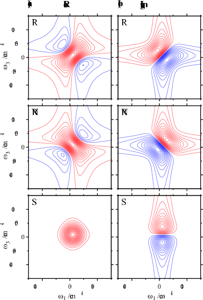
Figure 1: The stationary contributions (from top down) $S_{R}^{0}(\omega_{3},\omega_{1})$, $S_{NR}^{0}(\omega_{3},\omega_{1})$ and their sum $S^{0}(\omega_{3},\omega_{1})$ for the modulation by a low energy vibrational mode of $\omega=140$ cm^-1 and $\lambda=80$ cm^-1. The figures on the left present the real and the figures on the right the imaginary parts of the spectra, respectively. Apart from a slight asymmetry of the line-shapes with respect to the diagonal or anti-diagonal line, these figures represent very well the pure solvent line-shapes, too.

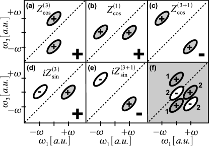
Figure 2: Demonstration of the construction of the 2D line-shape $S_{R}^{cos}(\omega_{3},\omega_{1})$. Real parts of the individual contributions are depicted in panels (a) to (e), together with the signs of the particular contributions. The total line-shape $S_{R}^{cos}(\omega_{3},\omega_{1})$ is depicted in panel (f). The central negative feature originates from the unshifted line shape $Z(\omega_{3},\omega_{1})$. The signs in the lower right corner in panels (a) to (e) represent the signs with which the diagrams contribute in Eq. (45). The numbers in panel (f) denote the predicted relative intensity of the features.

In this section, all calculations are performed assuming $T=300$ K and the bath correlation function in the form of an overdamped Brownian oscillator with reorganization energy $\lambda_{bath}=100$ cm^-1 and correlation time $\tau_{bath}=150$ fs. These numbers represent some characteristic values motivated by the molecular system studied in Paper I and Ref. Nemeth08a . For the Brownian oscillator model, the long time line-shape function has a constant term $g_{const}=-\lambda\tau_{c}(2k_{B}T\tau_{c}/\hbar-i)$ and a linear term, which can be written as $\bar{g}(t)=-g_{const}t/\tau_{c}$. The high temperature limit $k_{B}T\gg\hbar/\tau_{c}$ is valid for these parameters.

If the influence of vibrational modes converges to zero, i.e. for $\lambda/\omega\rightarrow 0$, the total spectrum is formed by the sum of the non-shifted rephasing shape $Z$ and the non-shifted non-rephasing shape $Y$. Qualitatively, these line-shapes are the same as those presented in Fig. 1. The real rephasing part of the spectrum has a characteristic orientation of the positive peak along the diagonal line, while the real non-rephasing part is elongated along the anti-diagonal line. Both line-shapes have negative “wings” stretching perpendicularly to the axis of elongation of the particular spectrum. If combined, they form a symmetric shape of the total response with solvent induced broadening only. The dispersive (imaginary) part of the solvent spectrum is also formed by the rephasing and non-rephasing elementary 2D line-shapes which are characterized by a nodal line parallel to the elongation axis of their real counterparts. Thus, the rephasing and non-rephasing dispersive parts differ from each other by the orientation of their nodal lines. The combined spectrum has a nodal line parallel to the $\omega_{1}$-axis.

The 2D line-shapes $Z$ and $Y$ represent the basic forms from which all spectral components can be constructed by means of a shift by the vibrational frequency $\omega$. We demonstrate this on the contribution $S_{R}^{cos}$ (cf. Eq. (45)). Fig. 2a-e depicts the individual terms in Eq. (45) according to Eqs. (41), (67) and (69), and 2(f) presents the total contribution $S_{R}^{cos}$. The oval shapes represent a single contour of the real part of the rephasing line-shape $Z$, thus showing their characteristic orientation and position in the spectrum. The numbers Fig. 2f represent the intensity of the corresponding spectral feature. Empty contours represent negative peaks, whereas shaded contours indicate positive peaks. From this schematic picture one can draw several conclusions. First, if the shift $\omega$ is small and all contributions overlap significantly, the positive part of the sum is elongated along the diagonal, with asymmetric negative parts along the anti-diagonal line. The negative features are stronger in the lower right corner of the 2D spectrum. Second, for vanishing $\omega$ the total contribution tends to zero, because all terms cancel. Consequently, for the same Huang-Rhys factor, the modulation by slower (lower energy) modes is weaker than the corresponding modulation by faster (higher energy) modes. Third, for $\omega$ larger than the width of the elementary line-shapes $Z$, the rephasing $cos$ contribution has the strongest positive feature on the right from the central frequency, a strong negative feature in the lower right corner, while in the center the contribution is negative. In the following sections we will demonstrate this prediction by numerical evaluation of Eqs. (42) to (48). Similar intuitive pictures can be created also for the non-rephasing spectra, using the pictorial representation of the line-shape $Y$.

We will distinguish between fast (high energy) and slow (low energy) vibrational modes relative to the inverse homogeneous spectral width $\Delta_{solv}$ (FWHM) of the solvent contribution. If $\omega\ll\Delta_{solv}$, i.e. vibrational crosspeaks in the 2D-FT spectrum or vibrational lines in the absorption spectrum would be indistinguishable, we assume the vibrational mode to be slow. The opposite case, $\omega\gg\Delta_{solv}$, characterizes fast vibrational modes for which individual vibrational features could be distinguished in optical spectra.

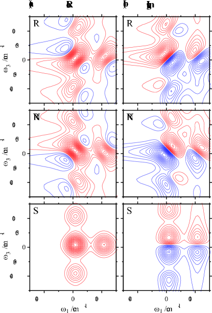
Figure 3: The stationary contributions (from top down) $S_{R}^{0}(\omega_{3},\omega_{1})$, $S_{NR}^{0}(\omega_{3},\omega_{1})$ and their sum $S^{0}(\omega_{3},\omega_{1})$ for the modulation by a high energy vibrational mode of $\omega=1000$ cm^-1and $\lambda=300$ cm^-1. The figures on the left present the real and the figures on the right the imaginary parts of the spectra, respectively.

Although the vibrational contribution is mostly dynamic, i.e. $t_{2}-$dependent, there is a certain time-independent contribution to the total 2D spectrum that originates from the vibrations. The stationary parts of the 2D spectra for modulation by a low energy vibrational mode of $\omega=140$ cm^-1 and a high energy vibrational mode of $\omega=1000$ fs are presented in Figs. 1 and 3, respectively. The reorganization energies have been set to $\lambda=80$ cm^-1 and $\lambda=300$ cm^-1, respectively. In case of the low energy mode, the shift of the line-shape by $\omega$ does not lead to any crosspeaks separated from the main diagonal peaks. The observed line-shape is only slightly broadened and distorted from the pure solvent line-shape by the vibrational contribution. In case of the high energy mode, we can distinguish separate vibrational cross- and diagonal peaks. In all cases we can identify the characteristic direction of elongation of the 2D line-shapes. The imaginary parts of all spectra also show characteristic orientations of the nodal lines. We can conclude that, in the static part of the 2D spectrum modulated by a high energy mode, the line-shapes are dictated by the chromophore solvent interaction, while the positions of the peaks are given by the vibrational frequency.

V.1 Modulation of 2D spectra by a low energy mode

The $t_{2}-$time evolution of the 2D spectra is mediated by the $\sin(\omega t_{2})$ and $\cos(\omega t_{2})$ functions which vary the magnitude of the contributions in Eqs. (44), (45), (47) and (48). A closer look at Eqs. (44) to (48) reveals that the rephasing and non-rephasing contributions have a very similar functional form. They differ mainly by the exchange $Z\longleftrightarrow Y$. Apart from this exchange, comparing the two $sin$ contributions, Eqs. (44) and (47), and the two $cos$ contributions, Eqs. (45) and (48), there is a flip of the sign in their first terms. This suggests that the rephasing and non-rephasing modulations of the total 2D shape differ not only in the orientation of their elongation, but also in phase. For $\cos\omega t_{2}=1$, the total rephasing contribution is at its maximum, while at the same time, the non-rephasing one is at its minimum. Due to the third term in Eqs. (44), (45), (47) and (48) this property is not exact. However, by studying diagrams similar to Fig. 2 for the various contributions, we have concluded that a $cos$ non-rephasing line-shape can be obtained from the rephasing one by turning the picture by $\pi/2$ anti-clockwise (corresponding to $Z\longleftrightarrow Y$ exchange), mirroring it by the diagonal line, and changing the sign.

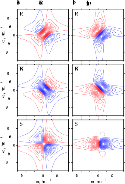
Figure 4: The $cos$ contribution for the modulation by a low energy vibrational mode of $\omega=140$ cm^-1. From top down: the rephasing and non-rephasing parts, and the sum spectrum. The figures on the left present the real and the figures on the right the imaginary parts of the spectra, respectively.

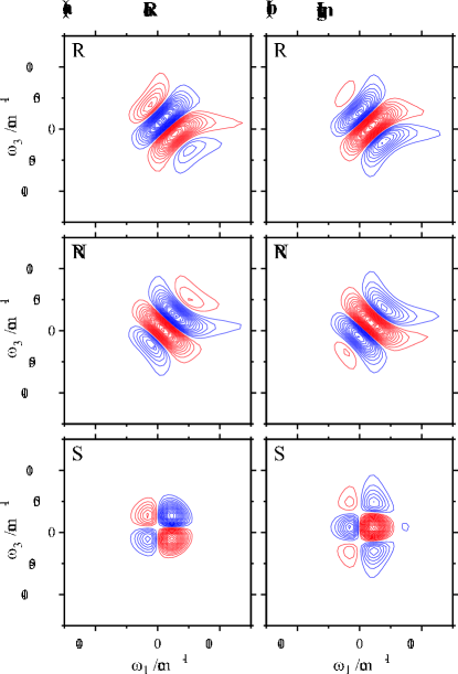
Figure 5: The $sin$ contribution for the modulation by a low energy vibrational mode of $\omega=140$ cm^-1. From top down: the rephasing and non-rephasing parts, and the sum spectrum. The figures on the left present the real and the figures on the right the imaginary parts of the spectra, respectively.

Figs. 4 and 5 present the $cos$ and $sin$ oscillating parts of the total 2D spectrum for modulation by a low energy vibrational mode. We can immediately notice that for both the $sin$ and the $cos$ modulation the real rephasing and non-rephasing contributions are approximately out of phase. For the set of parameters used here, the maximum amplitude of the $cos$ contribution is approximately twice the maximum amplitude of the $sin$ contribution, so that the $cos$ oscillation is the most significant feature in the $t_{2}$-evolution of the 2D spectrum. Neglecting therefore the $sin$ contribution for a while, we can predict a mutual out of phase modulation of the rephasing and non-rephasing parts of the 2D spectrum. This leads to the characteristic oscillation of the diagonal and anti-diagonal width of the total 2D spectrum (cf. Fig. 6), which was demonstrated experimentally in the preceding paper, Ref. Nemeth09a . The nodal line rotation in the dispersive part of the total 2D spectrum has a similar origin. As the rephasing and non-rephasing parts of the dispersive contribution have different orientation of their nodal lines, the total 2D spectrum exhibits oscillations of the nodal line angle, due to the change of relative amplitudes of rephasing and non-rephasing parts.

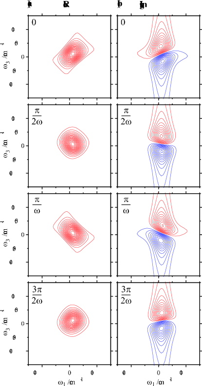
Figure 6: The time evolution of the total 2D spectrum of an electronic transition modulated by a low energy vibrational mode of $\omega=140$ cm^-1. From top down: 2D spectra at times $T=0,\mbox{$\frac{\pi}{2\omega}$, \mbox{$\frac{\pi}{\omega}$},}$ and $\frac{3\pi}{2\omega}$ fs. The figures on the left present the real and the figures on the right the imaginary parts of the spectra, respectively.

Fig. 6 demonstrates how the combined non-rephasing and rephasing signal gives rise to the characteristic experimentally observed modulation of the 2D line-shape. The results of our approximate analysis in this section are well confirmed by the experimental 2D spectra presented in Ref. Nemeth09a . Quantitative agreement with the experiment was achieved in Ref. Nemeth08a by modeling with the full expression for the corresponding response function, Eqs. (9) to (14).

V.2 Modulation of 2D spectra by a high energy mode

Encouraged by the successful comparison of the theory presented here with an experiment involving low energy vibrational modes, we can extend the treatment to high energy modes. For fast vibrational modes, where $\hbar\omega\gg 2k_{B}T$, the validity of the expansion in Eqs. (20) and (21) is limited only by the value of the Huang-Rhys factor $\lambda/\omega$, because $\coth(\hbar\omega/2k_{B}T)\approx 1$. The composition of different contributions to the 2D spectrum in this case, can be easily understood directly from considerations similar to those which led to Fig. 2. The rephasing real part of the $cos$ contribution shown in Fig. 7 corresponds very well to the depiction of Fig. 2f. A negative peak is present in the center of the spectrum, while two positive peaks are below the diagonal and one above the diagonal. The stronger of the two positive peaks below the diagonal is positioned at higher $\omega_{1}$ frequencies. All other contributions can be constructed in a similar way, including those oscillating with $sin(\omega t_{2})$ (cf. Fig. 8).

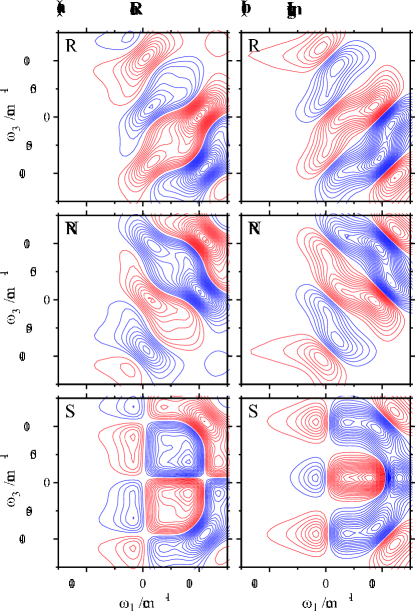
Figure 7: The $cos$ contribution for the modulation by a high energy vibrational mode of $\omega=1000$ cm^-1. From top down: the rephasing and non-rephasing parts, and the sum spectrum. The figures on the left present the real and the figures on the right the imaginary parts of the spectra, respectively.

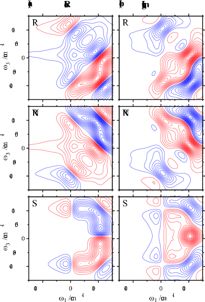
Figure 8: The $sin$ contribution for the modulation by a high energy vibrational mode of $\omega=1000$ cm^-1. From top down: the rephasing and non-rephasing parts, and the sum spectrum. The figures on the left present the real and the figures on the right the imaginary parts of the spectra, respectively.

Figure 9 presents the time evolution of the total 2D spectrum at different phases of the oscillation. An interesting observation is that for high energy vibrational modes the diagonal peaks oscillate with the opposite phases than in case of the low energy mode modulation, and with the opposite phase with respect to some of the cross-peaks. The shape of the $cos$ contributions for low and high energy mode modulations (Fig. 4 vs. Fig. 7), which are constructed from the same $Z$ and $Y$ but with different amount of shift from the transition frequency, again enables to understand the difference. Unlike the central diagonal peak, the crosspeaks oscillate between positive and negative values. The phase of these oscillations enables, for example, to clearly distinguish the 2D spectra in times $t_{2}=\pi/2\omega$ and $t_{2}=3\pi/2\omega$ by the real part of the spectrum only, without referring to the imaginary parts. For low energy modes, these two phases might be very difficult to distinguish.

The presence of negative features in different parts of the 2D-FT spectrum might influence the measured 2D-FT spectrum even if the spectrum of the pulse is not able to cover vibrational crosspeaks (see e.g. Ref. Nemeth09c ). However, sufficient information for the characterization of wavepacket motion cannot be obtained from such a measurement. If the experiment is performed with a laser pulse of a bandwidth comparable with the width of the vibrational peaks in the absorption or 2D spectrum (such as in Refs. Nemeth08a ; Nemeth09a and Nemeth09c ) the frequency of the laser pulse relative to the main diagonal peak determines the amount of influence the fast mode has on the 2D spectrum. In particular, in Refs. Nemeth08a ; Nemeth09a the central laser pulse frequency is lower than the position of the main diagonal peak, and the 2D spectrum is thus measured away from the fast vibrational features. Any vibrational modes with vibrational frequency significantly faster than the width of the laser pulse can thus be ignored from the evaluation, which was successfully done in Ref. Nemeth08a . On the other hand, if the laser pulse falls into the spectral region between the diagonal peaks, as is the case in Ref. Nemeth09c , the 2D spectrum is distorted by the high energy mode even if its frequency is larger that the width of the laser pulse.

Application of ultra broadband pulses that would cover significantly the whole region where a studied vibrational mode absorbs, promises to enable a complete characterization of the photo-induced vibrational wavepacket motion. Our results present reference spectra for an underdamped wavepacket motion in a harmonic potential. Distortions from this reference case can reveal changes in the shape of the wavepacket due to weak relaxation, anharmonicity, and also differences between the ground and excited state potential energy surfaces. From this point of view, 2D-FT experiments are of interest not only for molecules in solutions, but also for gas phase molecules, were they can characterize fundamental properties of vibrational DOF.

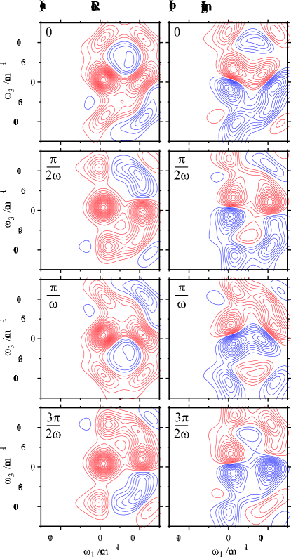
Figure 9: The time evolution of the 2D spectrum of an electronic transition modulated by a high energy vibrational mode of $\omega=1000$ cm^-1. From top down: 2D spectra at times $T=0,\mbox{$\frac{\pi}{2\omega}$, \mbox{$\frac{\pi}{\omega}$},}$ and $\frac{3\pi}{2\omega}$ fs. The figures on the left present the real and the figures on the right the imaginary parts of the spectra, respectively.

VI Conclusions

We have presented a qualitative theory of the time dependence of two-dimensional line-shapes of a two-level electronic system weakly coupled to a vibrational mode. We have studied the time evolution of the two-dimensional spectra in case of low and high energy vibrational modes and showed that the two-dimensional spectrum at $t_{2}$-times larger than the correlation time of the solvent can be qualitatively predicted based on the purely solvent two-dimensional line-shapes and knowledge of the vibrational frequency and Huang-Rhys factor. The theory predicts oscillations of the diagonal and anti-diagonal width of the two-dimensional spectrum caused by the rephasing and non-rephasing signals being modulated with opposite phase. In case of a low energy vibrational mode, the signal is predominantly modulated by a cosine term, as confirmed in the accompanying experimental paper. For high energy modes, where the line-shape width is smaller than the vibrational frequency, our theory predicts cross-peaks oscillating similarly to the low energy mode case, but the diagonal peaks oscillating with a phase opposite to the cross-peaks. Ultra broadband laser pulses would be necessary to observe high energy modes of molecules in liquid phases. However, in gas phase, a full characterization of vibrational motion based on two-dimensional spectroscopy would be possible.

Acknowledgements. T. M. acknowledges the kind support by the Czech Science Foundation through grant GACR 202/07/P278 and by the Ministry of Education, Youth, and Sports of the Czech Republic through research plan MSM0021620835. This work was supported by the Austrian Science Foundation (FWF) within the projects No. P18233 and F016/18 Advanced Light Sources (ADLIS). A.N. and J.S. thank the Austrian Academy of Sciences for partial financial support by the Doctoral Scholarship Programs (DOCfFORTE and DOC).

Appendix A Components of the vibrational response

In this appendix, we present explicite formulae for the components of the vibrational response, Eq. (22). The $t_{2}$-independent part $K_{n}(t_{1},t_{3})$ of Eq. (22) reads

$$K_{1}(t_{1},t_{3})=-i[\sin\omega t_{1}-\sin\omega t_{3}]$$

$$+\Xi(T)[\cos\omega t_{1}+\cos\omega t_{3}],$$ (49)

$$K_{2}(t_{1,}t_{3})=i[\sin\omega t_{1}+\sin\omega t_{3}]$$

$$+\Xi(T)[\cos\omega t_{1}+\cos\omega t_{3}],$$ (50)

$$K_{3}(t_{1},t_{3})=i[\sin\omega t_{1}-\sin\omega t_{3}]$$

$$+\Xi(T)[\cos\omega t_{1}+\cos\omega t_{3}],$$ (51)

$$K_{4}(t_{1},t_{3})=-i[\sin\omega t_{1}+\sin\omega t_{3}]$$

$$+\Xi(T)[\cos\omega t_{1}+\cos\omega t_{3}].$$ (52)

The cosine oscillating part $H_{n}(t_{1},t_{3})\cos\omega t_{2}$ of Eq. (22) can be written using

$$H_{1}(t_{1},t_{3})=\Xi(T)[1-\cos\omega t_{3}-\cos\omega t_{1}+\cos\omega(t_{1}+t_{3})]$$

$$+i[\sin\omega t_{1}-\sin\omega t_{3}-\sin\omega(t_{1}+t_{3})],$$ (53)

$$H_{2}(t_{1},t_{3})=-\Xi(T)[1-\cos\omega t_{3}-\cos\omega t_{1}+\cos\omega(t_{1}+t_{3})]$$

$$+i[\sin\omega t_{1}-\sin\omega t_{3}-\sin\omega(t_{1}+t_{3})],$$ (54)

$$H_{3}(t_{1},t_{3})=-\Xi(T)[1-\cos\omega t_{3}-\cos\omega t_{1}+\cos\omega(t_{1}+t_{3})]$$

$$+i[\sin\omega t_{1}+\sin\omega t_{3}-\sin\omega(t_{1}+t_{3})],$$ (55)

$$H_{4}(t_{1},t_{3})=\Xi(T)[1-\cos\omega t_{3}-\cos\omega t_{1}+\cos\omega(t_{1}+t_{3})]$$

$$+i[\sin\omega t_{1}+\sin\omega t_{3}-\sin\omega(t_{1}+t_{3})].$$ (56)

Finally, the sine oscillating part $G_{n}(t_{1},t_{3})\sin\omega t_{2}$ of Eq. (22) has a form of

$$G_{1}(t_{1},t_{3})=\Xi(T)[\sin\omega t_{3}+\sin\omega t_{1}-\sin\omega(t_{1}+t_{3})]$$

$$+i[1-\cos\omega t_{3}+\cos\omega t_{1}-\cos\omega(t_{1}+t_{3})],$$ (57)

$$G_{2}(t_{1},t_{3})=-\Xi(T)[\sin\omega t_{3}+\sin\omega t_{1}-\sin\omega(t_{1}+t_{3})]$$

$$+i[1-\cos\omega t_{3}+\cos\omega t_{1}-\cos\omega(t_{1}+t_{3})],$$ (58)

$$G_{3}(t_{1},t_{3})=-\Xi(T)[\sin\omega t_{3}+\sin\omega t_{1}-\sin\omega(t_{1}+t_{3})]$$

$$-i[1-\cos\omega t_{3}-\cos\omega t_{1}+\cos\omega(t_{1}+t_{3})],$$ (59)

$$G_{4}(t_{1},t_{3})=\Xi(T)[\sin\omega t_{3}+\sin\omega t_{1}-\sin\omega(t_{1}+t_{3})]$$

$$-i[1-\cos\omega t_{3}-\cos\omega t_{1}+\cos\omega(t_{1}+t_{3})].$$ (60)

Appendix B 2D line-shape components

This appendix lists some intermediate definitions used to derive Eqs. (43) to (48) for the time dependent 2D line-shapes. Line-shape components complementing Eq. (33) read

$$Z_{cos}^{(1)}(\omega_{3},\omega_{1})=FT_{2D}^{(-)}[e^{i(\omega_{eg}+\lambda)(t_{1}-t_{3})}$$

$$\times\bar{R}_{2}(t_{3},t_{1})\cos\omega t_{1}](\omega_{3},\omega_{1}),$$ (61)

$$Z_{sin}^{(3)}(\omega_{3},\omega_{1})=FT_{2D}^{(-)}[e^{i(\omega_{eg}+\lambda)(t_{1}-t_{3})}$$

$$\times\bar{R}_{2}(t_{3},t_{1})\sin\omega t_{3}](\omega_{3},\omega_{1}),$$ (62)

$$Z_{sin}^{(1)}(\omega_{3},\omega_{1})=FT_{2D}^{(-)}[e^{i(\omega_{eg}+\lambda)(t_{1}-t_{3})}$$

$$\times\bar{R}_{2}(t_{3},t_{1})\sin\omega t_{1}](\omega_{3},\omega_{1}),$$ (63)

$$Z_{cos}^{(3+1)}(\omega_{3},\omega_{1})=FT_{2D}^{(-)}[e^{i(\omega_{eg}+\lambda)(t_{1}-t_{3})}$$

$$\times\bar{R}_{2}(t_{3},t_{1})\cos\omega(t_{3}+t_{1})](\omega_{3},\omega_{1}),$$ (64)

$$Z_{sin}^{(3+1)}(\omega_{3},\omega_{1})=FT_{2D}^{(-)}[e^{i(\omega_{eg}+\lambda)(t_{1}-t_{3})}$$

$$\times\bar{R}_{2}(t_{3},t_{1})\sin\omega(t_{3}+t_{1})](\omega_{3},\omega_{1}).$$ (65)

Lineshape components complementing Eq. (41) read

$$Z_{cos}^{(1)}(\Omega_{3},\Omega_{1})=\frac{1}{2}\left(Z^{(0+)}+Z^{(0-)}\right),\;$$ (66)

$$Z_{sin}^{(1)}(\Omega_{3},\Omega_{1})=\frac{i}{2}\left(Z^{(0+)}-Z^{(0-)}\right),$$ (67)

$$Z_{cos}^{(3+1)}(\Omega_{3},\Omega_{1})=\frac{1}{2}\left(Z^{(+-)}+Z^{(-+)}\right),\;$$ (68)

$$Z_{sin}^{(3+1)}(\Omega_{3},\Omega_{1})=\frac{i}{2}\left(Z^{(-+)}-Z^{(+-)}\right),$$ (69)

$$Y_{cos}^{(3)}(\Omega_{3},\Omega_{1})=\frac{1}{2}\left(Y^{(+0)}+Y^{(-0)}\right),\;$$ (70)

$$Y_{sin}^{(3)}(\Omega_{3},\Omega_{1})=\frac{i}{2}\left(Y^{(-0)}-Y^{(+0)}\right),$$ (71)

$$Y_{cos}^{(1)}(\Omega_{3},\Omega_{1})=\frac{1}{2}\left(Y^{(0+)}+Y^{(0-)}\right),\;$$ (72)

$$Y_{sin}^{(1)}(\Omega_{3},\Omega_{1})=\frac{i}{2}\left(Y^{(0-)}-Y^{(0+)}\right),$$ (73)

$$Y_{cos}^{(3+1)}(\Omega_{3},\Omega_{1})=\frac{1}{2}\left(Y^{(++)}+Y^{(--)}\right),\;$$ (74)

$$Y_{sin}^{(3+1)}(\Omega_{3},\Omega_{1})=\frac{i}{2}\left(Y^{(--)}-Y^{(++)}\right).$$ (75)

References

- (1) Y. S. Kim and R. M. Hochstrasser, J. Phys. Chem. B 113, 8231 (2009).
- (2) C. J. Fecko, J. D. Eaves, J. J. Loparo, A. Tokmakoff, and P. L. Geissler, Science 301, 1698 (2003).
- (3) C. Kolano, J. Helbing, H. Kozinski, W. Sander, and P. Hamm, Nature 444, 469 (2006).
- (4) T. Brixner, T. Mančal, I. V. Stiopkin, and G. R. Fleming, J. Chem. Phys. 121, 4221 (2004).
- (5) A. Nemeth, F. Milota, T. Mančal, V. Lukeš, H. F. Kauffmann, and J. Sperling, Chem. Phys. Lett. 459, 94 (2008).
- (6) E. Collini and G. D. Scholes, Science 323, 369 (2009).
- (7) E. Collini and G. D. Scholes, J. Phys. Chem. A 113, 4223 (2009).
- (8) A. Nemeth, F. Milota, J. Sperling, D. Abramavicius, S. Mukamel, and H. F. Kauffmann, Chem. Phys. Lett. 469, 130 (2009).
- (9) T. Brixner, J. Stenger, H. M. Wasvani, M. Cho, R. E. Blankenship, and G. R. Fleming, Nature 434, 625 (2005).
- (10) D. Zigmantas, E. L. Read, T. Mančal, T. Brixner, A. T. Gardiner, R. J. Cogdell, and G. R. Fleming, P. Natl. Acad. Sci. USA 103, 12672 (2006).
- (11) G. S. Engel, T. R. Calhoun, E. L. Read, T.-K. Ahn, T. Mančal, Y.-C. Cheng, R. E. Blankenship, and G. R. Fleming, Nature 446, 782 (2007).
- (12) H. Lee, Y.-C. Cheng, and G. R. Fleming, Science 316, 1462 (2007).
- (13) K. W. Stone, K. Gundogdu, D. B. Turner, X. Li, S. T. Cundiff, and K. A. Nelson, Science 324, 1169 (2009).
- (14) D. M. Jonas, Annu. Rev. Phys. Chem. 54, 425 (2003).
- (15) M. H. Cho, H. M. Vaswani, T. Brixner, J. Stenger, and G. R. Fleming, J. Phys. Chem. B 109, 10542 (2005).
- (16) T. Mančal, A. Pisliakov, and G. R. Fleming, J. Chem. Phys. 124, 234504 (2006).
- (17) A. Pisliakov, T. Mančal, and G. R. Fleming, J. Chem. Phys. 124, 234505 (2006).
- (18) M. H. Cho, Chem. Rev. 108, 1331 (2008).
- (19) M. H. Cho and G. R. Fleming, J. Chem. Phys. 123, 114506 (2005).
- (20) P. Kjellberg, B. Brüggemann, and T. Pullerits, Phys. Rev. B 74, 024303 (2006).
- (21) B. Brüggemann, P. Kjellberg, and T. Pullerits, Chem. Phys. Lett 444, 192 (2007).
- (22) D. Abramavicius, B. Palmieri, and S. Mukamel, Chem. Phys. 357, 79 (2009).
- (23) D. Abramavicius, D. V. Voronine, and S. Mukamel, Biophys. J. 94, 3613 (2008).
- (24) Y.-C. Cheng, G. S. Engel, and G. R. Fleming, Chem. Phys. 341, 285 (2007).
- (25) Y.-C. Cheng and G. R. Fleming, J. Phys. Chem. A 112, 4254 (2008).
- (26) D. Egorova, M. F. Gelin, and W. Domcke, Chem. Phys. 341, 113 (2007).
- (27) D. Egorova, Chem. Phys. 347, 166 (2008).
- (28) G. D. Scholes, I. R. Gould, R. J. Cogdell, and G. R. Fleming, J. Phys. Chem. B 103, 2543 (1999).
- (29) A. Nemeth, F. Milota, T. Mančal, V. Lukeš, J. Hauer, H. F. Kauffmann, and J. Sperling, J. Chem. Phys. XX, YYYY (2010).
- (30) S. Mukamel, Principles of Nonlinear Spectroscopy (Oxford University Press, Oxford, 1995).
- (31) M. H. Cho, J.-Y. Yu, T. Joo, S. A. P. Y. Nagasawa, and G. R. Fleming, J. Phys. Chem. 100, 11944 (1996).
- (32) M. Yang and G. R. Fleming, J. Chem. Phys. 110, 2983 (1999).
- (33) T. Mančal and G. R. Fleming, J. Chem. Phys. 121, 10556 (2004).
- (34) A. Tokmakoff, J. Phys. Chem. A 104, 4247 (2000).
- (35) W. P. de Boeij, M. S. Pshenichnikov, and D. A. Wiersma, J. Phys. Chem. 100, 11806 (1996).
- (36) K. Lazonder, M. S. Pshenichnikov, and D. A. Wiersma, Opt. Lett. 31, 3354 (2006).
- (37) A. Nemeth, V. Lukeš, J. Sperling, F. Milota, H. F. Kauffmann, and T. Mančal, Phys. Chem. Chem. Phys. 11, 5986 (2009).