Polarization change induced by a galvanometric optical scanner

Abstract

We study the optical properties of a two-axis galvanometric optical scanner constituted by a pair of rotating planar mirrors, focusing our attention on the transformation induced on the polarization state of the input beam. We obtain the matrix that defines the transformation of the propagation direction of the beam and the Jones matrix that defines the transformation of the polarization state. Both matrices are expressed in terms of the rotation angles of two mirrors. Finally, we calculate the parameters of the general rotation in the Poincaré sphere that describes the change of polarization state for each mutual orientation of the mirrors.

1 Introduction

An optical scanner is a device constituted by two rotating planar mirrors which are used to deflect a laser beam along two perpendicular directions [1]. Among the different scanning techniques already developed, galvanometer-based scanners (galvos) offer flexibility, speed and accuracy at a relatively low cost. In fact, optical scanners based on the current galvo technology permit to obtain closed-loop bandwidths of several kHz and step response times in the 100 $\mu\mathrm{s}$ range even for beams with large radii. Moreover, a resolution at the $\mu\mathrm{rad}$ level can be achieved within a large scanning field, which is usually of the order of $20^{\circ}$.

Because of this superb properties, galvo scanners are the preferred solutions in many industrial and scientific applications requiring fast and precise beam steering capabilities, like medical imaging, information handling, laser display and material processing [2]. In addition, galvos could find potential applications in any practical context where the light beam which should be steered and/or stabilized with high precision also has a well defined state of polarization, like in interferometry with polarized light [3], in ellipsometry [4] or in polarization-sensitive optical coherence tomography [5]. Another important application might be in single-photon polarization-based quantum communications and quantum key distribution between two moving terminals, where a galvo scanner placed at the transmitter could be used to point and track the receiver with high accuracy. However, as the incidence angles of the beam with the two mirrors vary in function of their mutual position, the corresponding Fresnel coefficients [6] are subjected to a time-dependent change that affects the polarization state of the input beam. Therefore, in this kind of applications it is of primary importance to understand how the polarization state of the output beam changes in function of the combined motion of the mirrors.

The problem of the propagation of a polarized beam within a galvo scanner does not seem to have been treated before in the literature, since previous works were mainly aimed at studying beam path and image distortions [7, 8, 9, 10]. Moreover, previous studies of the changes of the polarization state caused by reflections of a light beam upon moving mirrors refer to optical configurations quite different from that of an optical scanner, like the Coudé focus of a telescope [11], sky scanners [12] and coelostats [13], or to more general cases of two-mirrors pointing and tracking systems [14, 15, 16]. For this reason, the principal purpose of the present work is to give a theoretical description of the effects on the polarization state of a light beam caused by the motion of the two mirrors of a galvo scanner.

This paper is structured as follows. In Section 2 we introduce the optical configuration of a galvo scanner and calculate the matrix that gives the propagation direction of the output beam. In Section 3 we obtain the Jones matrix of the galvo scanner. In Section 4 we discuss the polarization change under conditions of lossless mirrors, while in Section 5 we give a description in terms of rotation operators.

2 The galvo scanner

2.1 Optical scheme

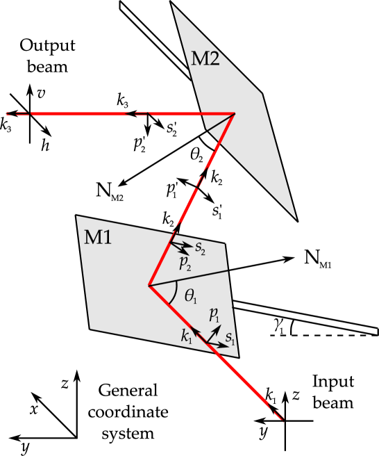
Figure 1: Schematic view of the galvo scanning system considered in this work, together with the general coordinate system and the unit vectors used in the calculations. An example of the optical path of a beam is indicated by the red line.

In general, a galvo scanner allows to control independently the direction of the output beam along two perpendicular axis by rotating the two mirrors about the axis of the corresponding galvanometers. We shall call these axis the “rotation axis” of the mirrors. The first mirror (M1) controls the deflection of the output beam along the horizontal direction (left/right), while the second mirror (M2) controls the deflection along the vertical direction (up/down). Both these deflections are usually referred to a predefined “zero position” of M1 and M2. Given a right-handed reference frame $(x,y,z)$, we consider the galvo mirrors to be at their zero positions when an input beam initially propagating along the positive $x$ axis will come out along the positive $y$ axis. According to this definition, the wave vector of the input beam is $\mathbf{k}_{1}=[1,0,0]$, while that of the output beam is $\mathbf{k}_{3}=[0,1,0]$.

The mutual orientation of the two mirrors when they are at the zero position is a critical parameter that defines the performances of a galvo scanner. In fact, the distance between their surfaces and the angular range of the scanning field usually requires the size of M2 to be larger than that of M1. Because of this, M2 is the component that strongly limits the speed of the entire scanning system.

In the simplest scheme of a galvo scanner, the rotation axis of M1 and M2 correspond with the positive $y$ axis and the negative $x$ axis, respectively. The zero position is achieved when the vector normal to the reflective surface of M1 is $[-\sqrt{2}/2,0,\sqrt{2}/2]$ and the vector normal to the surface of M2 is $[0,\sqrt{2}/2,-\sqrt{2}/2]$. Starting from this simple configuration, the optical design is usually optimized by rotating M1 by an angle $\gamma_{1}=15^{\circ}$ about the positive $x$ axis, as schematically shown in Fig. 1. This configuration presents the advantage to reduce both width and moment of inertia of M2 and reduce the overall size of the scanner, with only slight limitations on the speed with respect to the simple scheme. In the following, we will consider this optimized design because it is the most common configuration of current galvo scanners.

In order to find the zero positions of the mirrors, we have firstly to introduce the criterion to describe rotations that will be used throughout the paper. Any rotation by an angle $\vartheta$ about an axis $\mathbf{a}$ will be defined using the “right-hand rule”, such that a vector $\mathbf{v}$ rotates according to $\mathrm{d}\mathbf{v}=\mathbf{a}\times\mathbf{v}\,\mathrm{d}\vartheta$. For example, a rotation about the positive $x$ axis rotates $y$ toward $z$ and $z$ toward $-y$. According to this criterion, the zero position of M1 is obtained by starting from a configuration in which the normal to its surface is directed along the negative $x$ axis and, then, by rotating it by $45^{\circ}$ about the positive $y$ axis and by an angle $\gamma_{1}$ about the positive $x$ axis. It can be easily shown that the zero position of M2 is simply obtained, starting from a configuration in which the normal to its surface is directed along the positive $y$ axis, by rotating it about the positive $x$ axis by an angle $\gamma_{2}=45^{\circ}-\gamma_{1}/2=37.5^{\circ}$.

The deflection of the output beam along the $x$ axis (horizontal) is the result of a rotation of M1 by an angle $\alpha$ about its rotation axis, starting from its zero position. Therefore, the normal to the surface of M1 is generally defined by

$$\mathbf{N}_{\mathrm{M1}}=\left[\begin{array}[]{c}-\cos(\alpha+45^{\circ})\\ -\sin(\alpha+45^{\circ})\sin\gamma_{1}\\ \sin(\alpha+45^{\circ})\cos\gamma_{1}\end{array}\right]~{}.$$ (1)

Instead, the motion of the output beam along the $z$ axis (vertical) is achieved by rotating M2 by an angle $\beta$ about its rotation axis, starting from its zero position. In general, the normal to the surface of M2 has the following vectorial expression:

$$\mathbf{N}_{\mathrm{M2}}=\left[\begin{array}[]{c}0\\ \cos(\gamma_{2}+\beta)\\ -\sin(\gamma_{2}+\beta)\end{array}\right]~{}.$$ (2)

Obviously, when $\alpha\neq 0$ or $\beta\neq 0$, the propagation vector of the output beam, $\mathbf{k}_{3}$, is no longer parallel to the $y$ axis.

2.2 Geometrical transformation matrix

Before proceeding with the analysis of the polarization transformation we need to calculate the matrix that transforms the initial propagation direction $\mathbf{k}_{1}$ into the final one, $\mathbf{k}_{3}$. We assume that the mirrors are perfectly flat, with no deformation occurring while rotating. As a matter of fact, galvo mirrors are usually mass balanced about their centers of rotation. This solution presents the minimum polar moment of inertia and, therefore, permits to minimize the bending moments that are generated whenever an eccentric mass is rotated [2]. Under this condition, M1 and M2 have no dioptric power and the beam can be always considered as collimated throughout its propagation [7].

The reflection of a ray upon a mirror whose normal has components $[N_{x},N_{y},N_{z}]$ is generally described by the matrix [18]

$$\mathbf{R}=\left[\begin{array}[]{ccc}1-2N_{x}^{2}&-2N_{x}N_{y}&-2N_{x}N_{z}\\ -2N_{x}N_{y}&1-2N_{y}^{2}&-2N_{y}N_{z}\\ -2N_{x}N_{z}&-2N_{y}N_{z}&1-2N_{z}^{2}\end{array}\right]~{}.$$ (3)

Therefore, the reflection matrix associated to M1 is obtained by using the components of the normal vector shown in Eq. (1):

$$\footnotesize\mathbf{R}_{\mathrm{M1}}=\left[\begin{array}[]{ccc}\sin(2\alpha)&-\cos(2\alpha)\sin\gamma_{1}&\cos(2\alpha)\cos\gamma_{1}\\ -\cos(2\alpha)\sin\gamma_{1}&\cos^{2}\gamma_{1}-\sin(2\alpha)\sin^{2}\gamma_{1}&[1+\sin(2\alpha)]\cos\gamma_{1}\sin\gamma_{1}\\ \cos(2\alpha)\cos\gamma_{1}&[1+\sin(2\alpha)]\cos\gamma_{1}\sin\gamma_{1}&\sin^{2}\gamma_{1}-\sin(2\alpha)\cos^{2}\gamma_{1}\end{array}\right]~{}.$$ (4)

Instead, the reflection matrix of M2 is obtained by using the vector of Eq. (3):

$$\footnotesize\mathbf{R}_{\mathrm{M2}}=\left[\begin{array}[]{ccc}1&0&0\\ 0&-\cos[2(\gamma_{2}+\beta)]&\sin[2(\gamma_{2}+\beta)]\\ 0&\sin[2(\gamma_{2}+\beta)]&\cos[2(\gamma_{2}+\beta)]\end{array}\right]=\left[\begin{array}[]{ccc}1&0&0\\ 0&-\sin(\gamma_{1}+2\beta)&\cos(\gamma_{1}+2\beta)\\ 0&\cos(\gamma_{1}+2\beta)&\sin(\gamma_{1}+2\beta)\end{array}\right]~{}.$$ (5)

The transformation matrix of the galvo scanning system, i.e. the matrix $\mathbf{G}$ that maps $\mathbf{k}_{1}$ into $\mathbf{k}_{3}$, is finally given by the product between the reflection matrices of the two mirrors. Since any ray of the input beam is firstly reflected by M1 and then by M2, the $\mathbf{G}$ matrix is given by $\mathbf{G}=\mathbf{R}_{\mathrm{M2}}\,\mathbf{R}_{\mathrm{M1}}$, or

$$\scriptsize\mathbf{G}=\left[\begin{array}[]{ccc}\sin(2\alpha)&-\cos(2\alpha)\sin\gamma_{1}&\cos(2\alpha)\cos\gamma_{1}\\ \cos(2\alpha)\cos(2\beta)&\sin(2\alpha)\cos(2\beta)\sin\gamma_{1}-\sin(2\beta)\cos\gamma_{1}&-\sin(2\alpha)\cos(2\beta)\cos\gamma_{1}-\sin(2\beta)\sin\gamma_{1}\\ \cos(2\alpha)\sin(2\beta)&\sin(2\alpha)\sin(2\beta)\sin\gamma_{1}-\cos(2\beta)\cos\gamma_{1}&-\sin(2\alpha)\sin(2\beta)\cos\gamma_{1}-\cos(2\beta)\sin\gamma_{1}\end{array}\right]~{}.$$ (6)

This matrix clearly illustrates how the rotation of M1 results in a deflection of the output beam along the $x$ axis, while the rotation of M2 corresponds to a deflection along the $z$ axis. In fact, the final propagation vector of a beam initially propagating along the positive $x$ axis will be

$$\mathbf{k}_{3}=\left[\begin{array}[]{c}\sin(2\alpha)\\ \cos(2\alpha)\cos(2\beta)\\ \cos(2\alpha)\sin(2\beta)\end{array}\right]$$ (7)

According to the notation used here, a rotation of M1 by a positive (negative) $\alpha$ angle implies a deflection towards the positive (negative) $x$, while a rotation of M2 by a positive (negative) $\beta$ is related to a deflection towards the negative (positive) $z$.

3 Polarization transformation

The calculation of the polarization state of the output beam is made following a procedure quite similar to that explained in [14], which is essentially a polarization ray-tracing approach [17].

For a galvo scanner, the phenomenon which mainly affects the polarization of the output beam is the reflection upon the two mirrors. When the characteristics of a mirror are known, the effects on the polarization state of a light beam due to reflection can be treated using the Jones matrices and the Fresnel coefficients [6]. These coefficients give the amount of absorption and phase retard induced by the reflective element on the components of the electric field of the input beam along the parallel $(p)$ and perpendicular $(s)$ directions to the plane of incidence. Here we consider a mirror constituted by a single metallic surface with a complex refractive $\tilde{n}$, for simplicity. Assuming propagation through air, the Fresnel coefficients are defined as

$$r_{s}(\tilde{n},\theta_{i}) =-\frac{\sin(\theta_{i}-\theta_{t})}{\sin(\theta_{i}+\theta_{t})}~{},$$ (8)

$$r_{p}(\tilde{n},\theta_{i}) =\frac{\tan(\theta_{i}-\theta_{t})}{\tan(\theta_{i}+\theta_{t})}~{},$$ (9)

where $\theta_{i}$ is the incidence angle upon the mirror, $\sin\theta_{t}=(n_{0}\sin\theta_{i})/\tilde{n}$ and $n_{0}$ is the refractive index of the air. In Eq. (8) and (9) we have neglected the dependence of the refractive indexes on the wavelength because we are considering a laser beam with a very narrow spectral bandwidth.

We consider an input beam propagating along the direction $\mathbf{k}_{1}=[1,0,0]$. Its polarization plane coincides with the $(y,z)$ plane and the corresponding Jones vector is $\mathbf{E}_{1}=[E_{1y},E_{1z}]$, where the two components are in general complex. The beam intersects M1 with an angle of incidence $\theta_{1}$ given by the dot product

$$\cos\theta_{1}=\mathbf{k}_{1}\cdot\mathbf{N}_{\mathrm{M1}}$$ (10)

and, after being reflected, its direction of propagation is defined by the vector

$$\mathbf{k}_{2}=\mathbf{R}_{\mathrm{M1}}\mathbf{k}_{1}~{}.$$ (11)

Since the Fresnel coefficients are referred to the $p$ and $s$ directions with respect to the incidence plane, the Jones vector $\mathbf{E}_{1}$ has to be expressed in the $(p_{1},s_{1})$ basis relative the incidence plane with M1:

$$\mathbf{s}_{1}=\frac{\mathbf{k}_{1}\times\mathbf{k}_{2}}{\left|\mathbf{k}_{1}\times\mathbf{k}_{2}\right|}~{},\;\mathbf{p}_{1}=\frac{\mathbf{s}_{1}\times\mathbf{k}_{1}}{\left|\mathbf{s}_{1}\times\mathbf{k}_{1}\right|}~{}.$$ (12)

This change of basis is defined by a 2D rotation of the coordinate system:

$$\left[\begin{array}[]{c}E_{1p}\\ E_{1s}\end{array}\right]=\mathbf{R}(\eta_{0})\left[\begin{array}[]{c}E_{1y}\\ E_{1z}\end{array}\right]~{},$$ (13)

where

$$\mathbf{R}(\vartheta)=\left[\begin{array}[]{cc}\cos\vartheta&\sin\vartheta\\ -\sin\vartheta&\sin\vartheta\end{array}\right]$$ (14)

and $\eta_{0}$ is the angle subtended by $\mathbf{y}$ and $\mathbf{p}_{1}$.

In general, the $\phi$ angle subtended by two unit vectors $\mathbf{a}$ and $\mathbf{b}$ could be calculated by using the dot product $\cos\phi=\mathbf{a}\cdot\mathbf{b}$. However, the dot product just provides the smallest positive angle subtended by the two unit vectors and, therefore, the resulting $\phi$ would be found in the $[0,\pi]$ interval. To avoid this problem, we introduce the function $\mathrm{ang}(\mathbf{a},\mathbf{b})$ that provides the $\phi$ angle in the $[-\pi,\pi]$ range because it can discriminate between clockwise or counterclockwise rotations. In our case, vectors $\mathbf{a}$ and $\mathbf{b}$ lay in a plane perpendicular to the local propagation vector of the beam, $\mathbf{k}$. The $\mathrm{ang}$ function is defined as follows: after obtaining the vector

$$\mathbf{c}=\frac{\mathbf{a}\times\mathbf{b}}{\left|\mathbf{a}\times\mathbf{b}\right|}~{},$$ (15)

one has to calculate the scalar $u=\mathbf{c}\cdot\mathbf{k}$. It turns out that $u=1$ if the $\mathbf{c}$ and $\mathbf{k}$ vectors are parallel, or $u=-1$ if they are anti-parallel. The correct angle between $\mathbf{a}$ and $\mathbf{b}$ is finally given by

$$\phi=\mathrm{ang}(\mathbf{a},\mathbf{b})=u\arccos\left(\mathbf{a}\cdot\mathbf{b}\right)~{}.$$ (16)

According to this definition, the rotation angle in Eq. (13) is $\eta_{0}=\mathrm{ang}(\mathbf{y},\mathbf{p}_{1})$.

The $p$ and $s$ basis associated to the beam reflected by M1 is defined by the vectors

$$\mathbf{s}_{2}=\mathbf{s}_{1}~{},\;\mathbf{p}_{2}=\frac{\mathbf{s}_{2}\times\mathbf{k}_{2}}{\left|\mathbf{s}_{2}\times\mathbf{k}_{2}\right|}~{},$$ (17)

The Jones vector $\mathbf{E}_{2}=[E_{2p},E_{2s}]$ of this beam can be calculated using the Jones matrix of M1:

$$\left[\begin{array}[]{c}E_{2p}\\ E_{2s}\end{array}\right]=\left[\begin{array}[]{cc}r_{1p}(\tilde{n}_{1},\theta_{1})&0\\ 0&r_{1s}(\tilde{n}_{1},\theta_{1})\end{array}\right]\,\left[\begin{array}[]{c}E_{1p}\\ E_{1s}\end{array}\right]~{},$$ (18)

where $r_{1p}$ and $r_{1s}$ are the complex Fresnel coefficients for M1, while $\tilde{n}_{1}$ is its complex refractive index.

Then, the beam propagates along $\mathbf{k}_{2}$ and is reflected by the second mirror. In this case, the incidence angle is

$$\cos\theta_{2}=\mathbf{k}_{2}\cdot\mathbf{N}_{\mathrm{M2}}$$ (19)

and the final direction of propagation is given by

$$\mathbf{k}_{3}=\mathbf{R}_{\mathrm{M2}}\,\mathbf{k}_{2}=\mathbf{G}\,\mathbf{k}_{1}~{}.$$ (20)

The $p$ and $s$ vectors related to the reflection by M2 are

$$\mathbf{s}^{\prime}_{1}=\frac{\mathbf{k}_{2}\times\mathbf{k}_{3}}{\left|\mathbf{k}_{2}\times\mathbf{k}_{3}\right|}~{},\;\mathbf{p}^{\prime}_{1}=\frac{\mathbf{s}^{\prime}_{1}\times\mathbf{k}_{2}}{\left|\mathbf{s}^{\prime}_{1}\times\mathbf{k}_{2}\right|}~{},$$ (21)

for the incident beam, and

$$\mathbf{s}^{\prime}_{2}=\mathbf{s}^{\prime}_{1}~{},\;\mathbf{p}^{\prime}_{2}=\frac{\mathbf{s}^{\prime}_{2}\times\mathbf{k}_{2}}{\left|\mathbf{s}^{\prime}_{2}\times\mathbf{k}_{2}\right|}~{},$$ (22)

for the reflected beam. While propagating between M1 and M2, the Jones vector of the beam can be expressed in function of either the $(p_{2},s_{2})$ basis or the $(p^{\prime}_{1},s^{\prime}_{1})$ basis according to

$$\left[\begin{array}[]{c}E^{\prime}_{2p}\\ E^{\prime}_{2s}\end{array}\right]=\mathbf{R}(\eta_{1})\left[\begin{array}[]{c}E_{2p}\\ E_{2s}\end{array}\right]$$ (23)

where $\eta_{1}=\mathrm{ang}(\mathbf{p}_{2},\mathbf{p}^{\prime}_{1})$.

Finally, the $p$ and $s$ components of the Jones vector $\mathbf{E}_{3}$ associated to the output beam are given by

$$\left[\begin{array}[]{c}E_{3p}\\ E_{3s}\end{array}\right]=\left[\begin{array}[]{cc}r_{2p}(\tilde{n}_{2},\theta_{2})&0\\ 0&r_{2s}(\tilde{n}_{2},\theta_{2})\end{array}\right]\,\left[\begin{array}[]{c}E^{\prime}_{2p}\\ E^{\prime}_{2s}\end{array}\right]~{},$$ (24)

where $r_{2p}$ and $r_{2s}$ are the complex Fresnel coefficients for M2, while $\tilde{n}_{2}$ is its complex refractive index. It is useful to project $\mathbf{E}_{3}$ into a reference system defined by the local horizontal $(h)$ and vertical $(v)$ directions. The two unit vectors must form a left-handed reference frame together with $\mathbf{k}_{3}$:

$$\mathbf{h}=\frac{\mathbf{z}\times\mathbf{k}_{3}}{\left|\mathbf{z}\times\mathbf{k}_{3}\right|}~{},\;\mathbf{v}=\frac{\mathbf{k}_{3}\times\mathbf{h}}{\left|\mathbf{k}_{3}\times\mathbf{h}\right|}~{}.$$ (25)

Also in this case, the transformation from the $(p^{\prime}_{2},s^{\prime}_{2})$ basis to the $(h,v)$ basis is a 2D rotation:

$$\left[\begin{array}[]{c}E_{3h}\\ E_{3v}\end{array}\right]=\mathbf{R}(\eta_{2})\left[\begin{array}[]{c}E_{3p}\\ E_{3s}\end{array}\right]$$ (26)

where $\eta_{2}=\mathrm{ang}(\mathbf{p}^{\prime}_{2},\mathbf{h})$. All the unit vectors introduced in this Section have been drawn in Fig. 1 for clarity.

In summary, the Jones matrix describing the transformation of the polarization state of a collimated beam after passing through the galvo scanner is

$$\mathbf{M}=\left[\begin{array}[]{cc}\cos\eta_{2}&\sin\eta_{2}\\ -\sin\eta_{2}&\cos\eta_{2}\end{array}\right]\left[\begin{array}[]{cc}r_{2p}&0\\ 0&r_{2s}\end{array}\right]\times\\ \times\left[\begin{array}[]{cc}\cos\eta_{1}&\sin\eta_{1}\\ -\sin\eta_{1}&\cos\eta_{1}\end{array}\right]\left[\begin{array}[]{cc}r_{1p}&0\\ 0&r_{1s}\end{array}\right]\left[\begin{array}[]{cc}\cos\eta_{0}&\sin\eta_{0}\\ -\sin\eta_{0}&\cos\eta_{0}\end{array}\right]~{},$$ (27)

where we have dropped the explicit dependences on the refractive indexes and the incidence angles, for simplicity. Since the Fresnel coefficients of the Jones matrices shown in Eqs. (18) and (24) are in general complex, then both $E_{3h}$ and $E_{2v}$ will be complex and the final polarization state will be in general elliptical.

4 Lossless mirrors approximation

The Jones matrix of a galvo scanner shown in Eq. (27) is a product of rotation matrices and Jones matrices of mirrors. The latter have the following common form:

$$\mathbf{A}=\left[\begin{array}[]{cc}r_{p}&0\\ 0&r_{s}\end{array}\right]=\left[\begin{array}[]{cc}\rho_{p}\exp(\mathrm{i}\phi_{p})&0\\ 0&\rho_{s}\exp(\mathrm{i}\phi_{s})\end{array}\right]$$ (28)

where we have put in evidence the complex nature of the Fresnel coefficients $r_{p}$ and $r_{s}$. The determinant of this matrix $\det(\mathbf{A})=\rho_{p}\rho_{s}\exp[\mathrm{i}(\phi_{p}+\phi_{s})]$ is, in general, a complex number different from unity. For this reason, $\mathbf{A}$ is not unimodular unless $\rho_{p}\rho_{s}=1$ and $\phi_{p}=-\phi_{s}$. However, the $\mathbf{A}$ matrix can be always reduced to a product between a complex constant and an unimodular matrix:

$$\mathbf{A}=\sqrt{\rho_{p}\rho_{s}}\,\exp\left(\mathrm{i}\frac{\phi_{p}+\phi_{s}}{2}\right)\left[\begin{array}[]{cc}A\exp(\mathrm{i}\Phi)&0\\ 0&A^{-1}\exp(-\mathrm{i}\Phi)\end{array}\right]~{},$$ (29)

where $A=\sqrt{\rho_{p}/\rho_{s}}$ and $\Phi=(\phi_{p}-\phi_{s})/2$.

In the case of mirrors with a high reflectivity it is always found that $0.95\lesssim\rho_{p}/\rho_{s}\lesssim 1$ for a wide range of incidence angles [18]. Therefore, the $A$ factor can be approximated to unity (lossless mirrors) and the Jones matrix becomes totally equivalent to that of a simple phase retarder:

$$\mathbf{A}=\sqrt{\rho_{p}\rho_{s}}\,\exp\left(\mathrm{i}\frac{\phi_{p}+\phi_{s}}{2}\right)\left[\begin{array}[]{cc}\exp(\mathrm{i}\Phi)&0\\ 0&\exp(-\mathrm{i}\Phi)\end{array}\right]~{}.$$ (30)

We then assume that the two Jones matrix of the mirrors in Eq. (27) refer to the lossless case. Under this condition, neglecting the constant phase factor and the attenuation factor in Eq. (30), the approximated version of the Jones matrix of a galvo scanner is given by the product

$$\mathbf{M}\approx\left[\begin{array}[]{cc}\cos\eta_{2}&\sin\eta_{2}\\ -\sin\eta_{2}&\cos\eta_{2}\end{array}\right]\left[\begin{array}[]{cc}\exp(\mathrm{i}\Phi_{2})&0\\ 0&\exp(-\mathrm{i}\Phi_{2})\end{array}\right]\left[\begin{array}[]{cc}\cos\eta_{1}&\sin\eta_{1}\\ -\sin\eta_{1}&\cos\eta_{1}\end{array}\right]\times\\ \times\left[\begin{array}[]{cc}\exp(\mathrm{i}\Phi_{1})&0\\ 0&\exp(-\mathrm{i}\Phi_{1})\end{array}\right]\left[\begin{array}[]{cc}\cos\eta_{0}&\sin\eta_{0}\\ -\sin\eta_{0}&\cos\eta_{0}\end{array}\right]~{},$$ (31)

where $\Phi_{1}=(\phi_{1p}-\phi_{1s})/2$ and $\Phi_{2}=(\phi_{2p}-\phi_{2s})/2$.

The $\eta_{0}$ angle is defined as the $\mathrm{ang}$ function of the unit vectors $\mathbf{y}$, which is constant, and $\mathbf{p}_{1}$, which is a given by a vector triple product involving only $\mathbf{k}_{1}$ and $\mathbf{k}_{2}$. As shown in Eq. (11), $\mathbf{k}_{2}$ is the result of the product between the reflection matrix of M1 and $\mathbf{k}_{1}$, which is constant and coincides with the constant unit vector $\mathbf{x}$ in our assumptions. Therefore, $\eta_{0}$ only depends on $\mathbf{R}_{\mathrm{M1}}$, which is a function of the only $\alpha$ and $\gamma_{1}$ angles. Following a similar reasoning it can be shown that both $\eta_{1}$ and $\eta_{2}$ are functions of only $\alpha$, $\beta$ and $\gamma_{1}$.

The phase differences $\Phi_{1}$ and $\Phi_{2}$, instead, are related to the complex exponent of the the Fresnel coefficients, which depends on the complex refractive indexes of the mirrors and the incidence angles. According to the definitions given in Eq. (10) and (19), $\theta_{1}$ is a function of the constant vector $\mathbf{k}_{1}$ and the normal vector to M1, while $\theta_{2}$ is a function of $\mathbf{k}_{2}$ and the normal vector to M2. As a result, we have $\Phi_{1}=\Phi_{1}(\tilde{n}_{1},\alpha,\gamma_{1})$ and $\Phi_{2}=\Phi_{2}(\tilde{n}_{2},\alpha,\beta,\gamma_{1})$.

If the input beam is always kept at a fixed direction and the mechanical properties of the galvo scanner do not change with time, which means constant values of $\gamma_{1}$ and of the complex refractive indexes of the mirrors, then the $\mathbf{M}$ matrix is just a function of the $\alpha$ and $\beta$ angles.

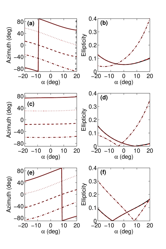
Figure 2: Azimuth and ellipticity of output polarization states from a galvo scanner. (a) and (b): $\beta=-20^{\circ}$; (c) and (d): $\beta=0^{\circ}$; (e) and (f): $\beta=+20^{\circ}$. Black lines refer to the output states calculated using the Jones matrix of Eq. (27), while red lines have been obtained assuming lossless mirrors. The polarization states of the input beam are $H$ (solid lines), $V$ (dashed lines), +45 (dash-dotted lines) and -45 (dotted lines). In the right panels, dashed lines appear superimposed on solid lines, while dotted lines appear superimposed on dash-dotted lines.

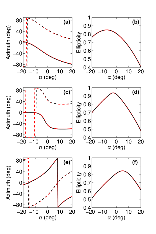
Figure 3: Azimuth and ellipticity of output polarization states from a galvo scanner. (a) and (b): $\beta=-20^{\circ}$; (c) and (d): $\beta=0^{\circ}$; (e) and (f): $\beta=+20^{\circ}$. Black lines refer to the output states calculated using the Jones matrix of Eq. (27), while red lines have been obtained assuming lossless mirrors. The polarization states of the input beam are $R$ (solid lines), and $L$ (dashed lines). In the right panels, all lines appear superimposed.

As an useful example, we consider a galvo scanner with bare silver mirrors and a collimated laser beam at 850 nm. Since both M1 and M2 are made of the same material, they also have the same complex refractive index $\tilde{n}=0.152+5.678\,\mathrm{i}$ at that wavelength [19]. We then take a number of polarization states of the input beam and calculate the corresponding final state obtained by varying the rotation angles $\alpha$ and $\beta$ of M1 and M2 in the range $[-20^{\circ},20^{\circ}]$ with steps of $0.1^{\circ}$. The polarization states of the input beam are chosen in order to fill as much as possible the Poincaré sphere, which means ellipticity in the range $[-1,1]$ with steps of 0.01 and azimuth in the range $[-90^{\circ},90^{\circ}]$ with steps of $1.8^{\circ}$.

For each initial state and for each mutual position of the galvo mirrors, we obtain the exact output state by using the Jones matrix of Eq. (27), as well as the approximated version provided by Eq. (31). In Fig. 2 we show the azimuth and the ellipticity of the output states obtained considering four linear polarization states of the input beam (ellipticity equal to zero), i.e. horizontal ($H$, $\mathbf{E}_{1}=[1,0]$), vertical ($V$, $\mathbf{E}_{1}=[0,1]$), linear at $45^{\circ}$ (45, $\mathbf{E}_{1}=[1,1]/\sqrt{2}$), linear at $-45^{\circ}$ (-45, $\mathbf{E}_{1}=[1,-1]/\sqrt{2}$), while in Fig. 3 we report the values obtained using right circular ($R$, $\mathbf{E}_{1}=[1,-\mathrm{i}]/\sqrt{2}$) and left circular ($L$, $\mathbf{E}_{1}=[1,\mathrm{i}]/\sqrt{2}$) initial states (ellipticity equal to one). Both Figures show the exact output states and the corresponding approximated version, for comparison.

In order to define the degree of reliability of the lossless mirror approximation, we calculate the absolute value of the difference between azimuth and ellipticity of the states obtained by using the two versions of the Jones matrix. We find that the absolute value of the difference between the azimuth is typically lower than $\sim 0.8^{\circ}$, while the absolute value of the difference between the ellipticity is typically lower than $\sim 5\times 10^{-3}$. For this reason, black and red curves related to the same initial polarization state appear almost perfectly superimposed in Fig. 2 and 3. However, the lossless mirror approximation cannot be used if the output polarization state is close to circular. Under this condition and for particular combinations of the $\alpha$ and $\beta$ angle there might a large discrepancy (even more than $10^{\circ}$) between the azimuth of exact and approximated states.

5 Rotation operators

Following a notation commonly used in quantum mechanics, the approximated Jones matrix of a galvo scanner [Eq. (31)] can be represented as a product of rotation operators [20]:

$$\mathbf{M}\approx\exp(-\mathrm{i}\sigma_{y}\eta_{2})\,\exp(\mathrm{i}\sigma_{z}\Phi_{2})\,\exp(-\mathrm{i}\sigma_{y}\eta_{1})\,\exp(\mathrm{i}\sigma_{z}\Phi_{1})\,\exp(-\mathrm{i}\sigma_{y}\eta_{0})~{},$$ (32)

where the Pauli matrices are

$$\sigma_{x}=\left[\begin{array}[]{cc}0&1\\ 1&0\end{array}\right]~{},\;\sigma_{y}=\left[\begin{array}[]{cc}0&-\mathrm{i}\\ \mathrm{i}&0\end{array}\right]~{},\;\sigma_{z}=\left[\begin{array}[]{cc}1&0\\ 0&-1\end{array}\right]~{}.$$ (33)

For this reason, the $\mathbf{M}$ matrix is unitary and unimodular.

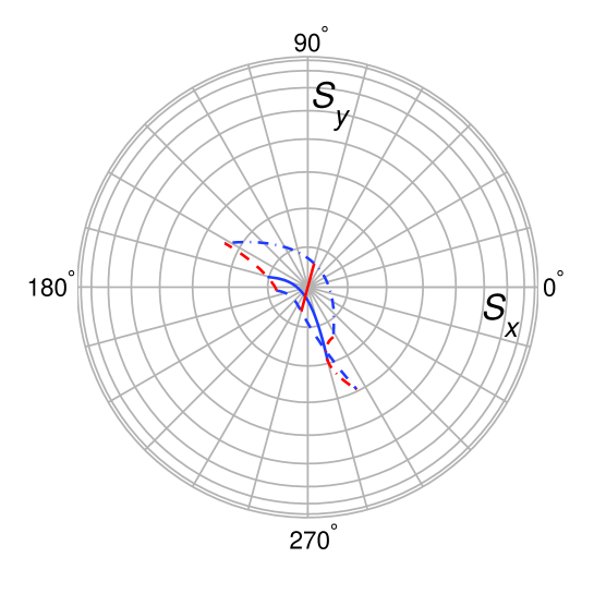
Figure 4: Traces of the direction of the rotation axis associated to the Jones matrix of a galvo scanner as a function of the $\alpha$ and $\beta$ angles. The lines are traced on the surface of the Poincaré sphere, whose bottom part is depicted with a gray grid. Radial lines correspond to meridians drawn at $15^{\circ}$ intervals, while circles corresponds to parallels drawn at $10^{\circ}$ intervals starting from the south pole. Blue lines refer to a fixed $\beta$ ($\beta=-20^{\circ}$ dashed line, $\beta=0^{\circ}$ solid line, $\beta=20^{\circ}$ dash dotted) and $-20^{\circ}\leq\alpha\leq 20^{\circ}$, while red lines refer to a fixed $\alpha$ ($\alpha=-20^{\circ}$ dashed line, $\alpha=0^{\circ}$ solid line, $\alpha=20^{\circ}$ dash dotted) and $-20^{\circ}\leq\beta\leq 20^{\circ}$.

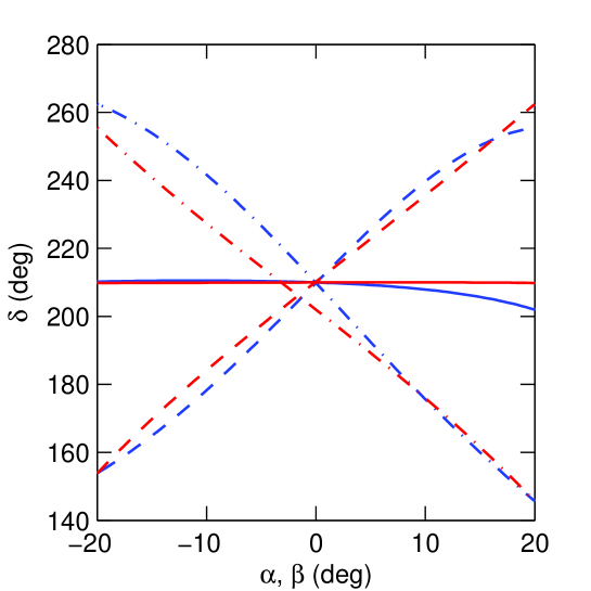
Figure 5: Rotation angle $\delta$ associated to the Jones matrix of a galvo scanner as a function of the $\alpha$ and $\beta$ angles. Blue lines refer to a fixed $\beta$ ($\beta=-20^{\circ}$ dashed line, $\beta=0^{\circ}$ solid line, $\beta=20^{\circ}$ dash dotted) and $-20^{\circ}\leq\alpha\leq 20^{\circ}$, while red lines refer to a fixed $\alpha$ ($\alpha=-20^{\circ}$ dashed line, $\alpha=0^{\circ}$ solid line, $\alpha=20^{\circ}$ dash dotted) and $-20^{\circ}\leq\beta\leq 20^{\circ}$.

It is well known that any unitary and unimodular matrix $\mathbf{U}$ represents a rotation on the Poincaré sphere:

$$\mathbf{U}=\exp\left(-\mathrm{i}\mathbf{n}\cdot\boldsymbol{\sigma}\frac{\delta}{2}\right)~{},$$ (34)

where $\boldsymbol{\sigma}=[\sigma_{x},\sigma_{y},\sigma_{z}]$, $\mathbf{n}=[\sin\vartheta\cos\varphi,\sin\vartheta\sin\varphi,\cos\vartheta]$ is an unit vector defining the rotation axis ($\varphi$ is the longitude and $\vartheta$ is the latitude) and $\delta$ is the rotation angle about $\mathbf{n}$. The $\mathbf{U}$ matrix can be always expressed in terms of a constant $a_{0}$ and a vector $\mathbf{a}=[a_{x},a_{y},a_{z}]$ as

$$\mathbf{U}=a_{0}\mathbf{1}+\mathrm{i}\mathbf{a}\cdot\boldsymbol{\sigma}=\left[\begin{array}[]{cc}a_{0}+\mathrm{i}a_{z}&\mathrm{i}a_{x}+a_{y}\\ \mathrm{i}a_{x}-a_{y}&a_{0}-\mathrm{i}a_{z}\end{array}\right]~{},$$ (35)

where $\mathbf{1}$ is the identity matrix, $a_{0}=\cos(\delta/2)$, $|\mathbf{a}|=\sin(\delta/2)$ and $\mathbf{n}=\mathbf{a}/|\mathbf{a}|$. The transformation matrix of the galvo scanner expressed in Eq. (31) can be decomposed according to this scheme, thus giving:

$$\left\{\begin{aligned} a_{0}&=-\sin\Phi_{1}\sin\Phi_{2}\cos(\eta_{0}-\eta_{1}+\eta_{2})+\cos\Phi_{1}\cos\Phi_{2}\cos(\eta_{0}+\eta_{1}+\eta_{2})\\ a_{x}&=-\sin\Phi_{1}\cos\Phi_{2}\sin(\eta_{0}-\eta_{1}-\eta_{2})-\cos\Phi_{1}\sin\Phi_{2}\sin(\eta_{0}+\eta_{1}-\eta_{2})\\ a_{y}&=-\cos\Phi_{1}\cos\Phi_{2}\sin(\eta_{0}+\eta_{1}+\eta_{2})+\sin\Phi_{1}\sin\Phi_{2}\sin(\eta_{0}-\eta_{1}+\eta_{2})\\ a_{z}&=\sin\Phi_{1}\cos\Phi_{2}\cos(\eta_{0}-\eta_{1}-\eta_{2})+\cos\Phi_{1}\sin\Phi_{2}\cos(\eta_{0}+\eta_{1}-\eta_{2})\end{aligned}\right.~{}.$$ (36)

For each configuration of the two mirrors of the galvo scanner, i.e. for each pair of rotation angles $\alpha$ and $\beta$, Eq. (36) can be used to calculate the instantaneous rotation axis $\mathbf{n}$ and the corresponding rotation angle $\delta$ that define the transformation of the polarization state of the input beam.

Figs. 4 and 5 show the results obtained by considering a galvo scanner with the characteristics described in Sect. 4 for various combinations of $\alpha$ and $\beta$. Note that the instantaneous rotation axis coincides with the negative $z$ axis for $\alpha=0^{\circ}$ and $\beta=7.5^{\circ}$.

6 Conclusions

We have studied the optical properties of a two-axis galvanometric optical scanner in order to understand how the polarization state of an input beam changes at the output of the system. We obtained the transformation matrix that maps the propagation direction of the input beam into the propagation direction of the output beam, as well as the Jones matrix that maps the initial polarization state into the final one. Both these matrices have been expressed in function of the rotation angles $\alpha$ and $\beta$, therefore permitting to predict the output polarization state for any allowed position of two galvo mirrors. This change corresponds to a general rotation of the polarization state in the Poincaré sphere, where both the instantaneous rotation axis and the rotation angle are both functions of the $\alpha$ and $\beta$ angles.

Although the numerical results presented here has been obtained by considering a particular orientation of the two galvo mirrors in their zero position, the analytical expressions can also be applied also to any other configuration of the optical scanner simply by using the appropriate normal vectors, as well as to any kind of mirror having protection coating by using the appropriate form of the Fresnel coefficients.

References

- [1] J. D. Zook, Light beam deflector performance: a comparative analysis. Applied Opt. 13, 875–887 (1974).
- [2] G. F. Marshall, Handbook of optical and laser scanning. (CRC Press, 2004).
- [3] P. Hariharan, Optical interferometry, 2nd ed. (Academic Press, 2003).
- [4] R. M. A. Azzam and N. M. Bashara, Ellipsometry and polarized light. (North-Holland Publ. Co., 1977).
- [5] W. Drexler and J. G. Fujimoto, Optical Coherence Tomography: Technology and Applications. (Springer, 2008).
- [6] M. Born and E. Wolf, Principles of Optics (Cambridge University Press, 1999).
- [7] Y. Li and J. Katz, Laser beam scanning by rotary mirrors. I. Modeling mirror-scanning devices. Applied Opt. 34, 6403–6416 (1995).
- [8] Y. Li, Laser beam scanning by rotary mirrors. II. Conic-section scan patterns. Applied Opt. 34, 6417–6430 (1995).
- [9] J. Xie, S. Huang, Z. Duan, Y. Shi, and S. Wen, Correction of the image distortion for laser galvanometric scanning system. Opt. Laser Technol. 37, 305–311 (2005).
- [10] Y. Li, Beam deflection and scanning by two-mirror and two-axis systems of different architectures: a unified approach. Applied Opt. 47, 5976–5985 (2008).
- [11] E. F. Borra, Polarimetry at the coude focus - Instrumental effects. Publ. Astron. Soc. Pacific 88, 548–556 (1976).
- [12] L. M. Garrison, Z. Blaszczak, and A. E. S. Green, Polarization characteristics of an altazimuth sky scanner. Applied Opt. 19, 1419–1424 (1980).
- [13] C. Beck, R. Schlichenmaier, M. Collados, L. Bellot Rubio, and T. Kentischer, A polarization model for the German Vacuum Tower Telescope from in situ and laboratory measurements. Astron. Astrophys. 443, 1047–1053 (2005).
- [14] C. Bonato, M. Aspelmeyer, T. Jennewein, C. Pernechele, P. Villoresi, and A. Zeilinger, Influence of satellite motion on polarization qubits in a Space-Earth quantum communication link. Opt. Expr. 14, 10050–10059 (2006).
- [15] C. Bonato, C. Pernechele, and P. Villoresi, Influence of all-reflective optical systems in the transmission of polarization-encoded qubits. J. Opt. Soc. Am. A 9, 899–906 (2007).
- [16] C. Bonato, A. Tomaello, V. Da Deppo, G. Naletto, and P. Villoresi, Feasibility of satellite quantum key distribution. New J. Phys. 11, 045017 (2009).
- [17] R. A. Chipman, Mechanics of polarization ray tracing. Opt. Engineering 34, 1636–1645 (1995).
- [18] M. Bass, E. W. V. Stryland, D. R. Williams, and W. L. Wolfe, Handbook of Optics. Volume I: Fundamentals, Techniques, and Design. (McGraw-Hill Inc., 1995).
- [19] E. D. Palik, Handbook of optical constants of solids. (Academic Press, 1991).
- [20] J. J. Sakurai, Modern quantum mechanics (Addison Wesley, 1985).