A hybrid MPI-OpenMP scheme for scalable parallel pseudospectral computations for fluid turbulence

Abstract

A hybrid scheme that utilizes MPI for distributed memory parallelism and OpenMP for shared memory parallelism is presented. The work is motivated by the desire to achieve exceptionally high Reynolds numbers in pseudospectral computations of fluid turbulence on emerging petascale, high core-count, massively parallel processing systems. The hybrid implementation derives from and augments a well-tested scalable MPI-parallelized pseudospectral code. The hybrid paradigm leads to a new picture for the domain decomposition of the pseudospectral grids, which is helpful in understanding, among other things, the 3D transpose of the global data that is necessary for the parallel fast Fourier transforms that are the central component of the numerical discretizations. Details of the hybrid implementation are provided, and performance tests illustrate the utility of the method. It is shown that the hybrid scheme achieves near ideal scalability up to $\sim 20000$ compute cores with a maximum mean efficiency of 83%. Data are presented that demonstrate how to choose the optimal number of MPI processes and OpenMP threads in order to optimize code performance on two different platforms.

1 Introduction

Fluid turbulence arises from interactions at all spatial and temporal scales, and is therefore the quintessential petascale application. The Reynolds number ${\sf{R_{v}}}$, which measures the strength of the nonlinearity in turbulent fluid systems, determines the number of degrees of freedom (d.o.f.) required to resolve all spatial scales, which increases as ${\sf{R_{v}}}^{9/4}$ (in the Kolmogorov framework [11, 10]). For geophysical flows, ${\sf{R_{v}}}$ is often greater than $10^{8}$, suggesting the need to evolve the geo-fluid equations with greater than $10^{18}$ grid points, if completely accurate computations of turbulent geophysical flows are to be realized without resorting to modeling of unresolved scales. This approach to computing fluid flows in which all spatial and temporal scales are resolved is called direct numerical simulation (DNS). If the goal is to simulate geophysical flows accurately, such computations must be carried out at exascale resolutions, which are not currently feasible. But petascale resolutions are just now becoming available, that can accommodate resolutions of $10^{15}$ grid points, corresponding to ${\sf{R_{v}}}\sim 10^{7}$, which still allows for sufficient scale separation to study physically relevant complex turbulent flows.

Pseudospectral methods provide a very useful tool to study the problem because of their computational efficiency and high order numerical convergence. Attention is often focused on a $2\pi$–periodic box domain in order to study scale interaction as it allows the use of fast spectral transforms that have a computational complexity of $\sim N\log(N)$ instead of $\sim N^{2}$, where $N$ is the linear resolution. For studies of homogeneous and isotropic turbulence, this choice is entirely consistent because the domain preserves the underlying translational and rotational invariance of the physics. But the approach is useful as well for studies of anisotropic or inhomogeneous turbulence, which broadens its usefulness. On the periodic domain, the Fourier basis is optimal, and the pseudospectral discretization [1, 7, 8] is pre-eminent due to the effectiveness of the fast Fourier transform (FFT) in converting from configuration to spectral space, and back again. The pseudospectral method [12] has thus been used extensively in studies of computational fluid dynamics (CFD) including turbulence, with references too numerous to cite. This method has the extra advantage of accurately capturing the interaction of multiple scales with little or no numerical dissipation or dispersion. This is clearly an important property for the numerics if we wish to quantify small scale dissipative effects that arise in the context of nonlinear turbulent interactions.

Pseudospectral methods, however, require global spectral transforms, and, therefore, are hard to implement in distributed memory environments. This has been labeled a crucial limitation of the method until domain decomposition techniques arose that allowed computation of serial FFTs in different directions in space (local in memory) after performing transpositions. One of these methods is the 1D (slab) domain decomposition (see e.g., [2]), that enables multidimensional FFTs to be parallelized effectively using the Message Passing Interface (MPI). However, these methods are often limited in the number of processors that can be used, and generalizations to larger processor counts using solely MPI are often expensive or hard to tune as transpositions require all-to-all communications. Also, multi-dimensional transforms of some non-Fourier basis, such as spherical harmonics, cannot be parallelized using this technique. In the present work, a hybrid (MPI-OpenMP) scheme is described that builds upon the existing domain decomposition scheme that has been shown to be effective for parallel scaling using MPI alone. We leverage this existing domain decomposition method in constructing a hybrid MPI-OpenMP model using loop–level OpenMP directives and multi-threaded FFTs. The implementation is intended to address several concerns: It addresses the multi—level architectures of emerging platforms; and it is also designed to be portable to a variety of systems, with the expectation that it will provide scalability and performance without detailed knowledge of network topology or cache structure.

The idea of such loop-level–or implicit–parallelization in concert with MPI is not new. To date, these have generally been attempted on small core count systems, and the pure MPI scheme is found to outperform the hybrid schemes. In the context of CFD applications, it was found that on core counts up to 256 processors the overall elapsed time (for a finite element solver) was better for the pure MPI scheme than for the hybrid, even though the hybrid approach showed improved communication times in some cases [16]. A hybrid approach was taken in an implementation of a parallel 3D FFT algorithm [14] that succeeded in reducing the number of cache misses in the algorithm on an SMP system. But this approach was again tested only on a small core count platform, and considered the FFT algorithm alone, without the full fluid solver. To the best of our knowledge, the scheme described herein is the first published implementation of a hybrid model in a pseudospectral CFD context that has been attempted on high core count systems, and found to scale well.

In the following sections we present a new hybrid implementation. We begin first with a description (Section 2) of the numerical method and the underlying domain decomposition scheme. In Section 3 the hybrid model is presented, and a new domain decomposition picture is offered for viewing the distribution of work on multicore nodes. We also discuss in this section the implementation of the loop–level parallelization. Benchmarks are provided in Section 4, where we also consider the overhead and performance of the OpenMP parallelization, and the scalability of the full hybrid formulation. Finally, in Section 5, we offer some concluding remarks on lessons learned and our expectations for future hybrid performance on petascale systems.

2 The pseudo-spectral method and the underlying domain decomposition

All of the work in this paper will be based on simulations of the Navier–Stokes equations:

$$\partial_{t}{{\mathbf{u}}}+{{\mathbf{u}}}\cdot\nabla{{\mathbf{u}}}=-\nabla p+\nu\nabla^{2}{{\mathbf{u}}},$$ (1)

$$\nabla\cdot{{\mathbf{u}}}=0,$$ (2)

where ${\mathbf{u}}$ is the velocity, the kinematic viscosity is $\nu$, and the pressure, $p$, can be viewed as a Lagrange variable used to satisfy the incompressibility constraint, (Eq. 2). These equations are solved using a pseudo-spectral method [1, 7, 8, 13], in which each component of ${\mathbf{u}}$ is represented as a truncated (Galerkin) expansion in terms of the Fourier basis, and the nonlinear term is computed in physical space and then transformed using the fast Fourier transform (FFT), to spectral space. The nonlinear term is computed in such a way that the velocity is projected onto a divergence-free space, in order to satisfy (Eq. 2). Details of this projection and of the dealiasing required by the action of the nonlinear term are not central to the discussion and can be found elsewhere [1, 13], as can additional details of the discretization and parallelization of the scheme using solely MPI [6].

Figure 1: Underlying 1D (slab) domain decomposition for pseudo-spectral method (left). Each processor works on a slab of size $N\times N\times M$, where $M=N/P$. The FFT is done by first doing the FFTs locally in each slab, in the directions specified by the arrows, yielding partially transformed data of size $N/2+1\times N\times M$. Then, an all-to-all communication is done to transpose the data globally (right), so that the remaining 1D FFT can be done in the direction specified by the arrow. The data for this step is stored in a cube of size $N/2+1\times N\times N$, and each processor now computes the FFT locally in a slab of size $P=(N/2+1)/P$. [Figure adapted from [6].]

The key piece of any pseudospectral method, particularly for parallel computing, is the multidimensional Fourier transform algorithm. An efficient parallel implementation of this algorithm is essential for attaining high Reynolds numbers in turbulent hydrodynamics simulations, which is of chief concern here. We focus on a 3D Fourier transform of a scalar (or vector component) field of size $N^{3}$, with $N$ nodes in each coordinate direction of the $2\pi$-periodic domain. The distribution of real space points can be viewed as a cubic array of $N^{3}$ real numbers. In the underlying domain decomposition each processor receives a “slab” of size $N\times N\times M$ node points, where $M=N/N_{P}$, and $N_{P}$ is the number of processors. This is referred to as a 1D domain decomposition because the distribution to processors occurs in one direction only; this decomposition is visualized in Fig. 1. Fourier transforms are performed locally in the direction of the arrows on the slab owned by a processor. The partially transformed (complex) data resides in a cube of size $(N/2+1)\times N\times M$. The reduction in the size of the array results from the fact that a Fourier transform of real data $u(x)$ satisfies $\hat{u}(k)=-\hat{u}^{*}(k)$ (where the asterisk denotes complex conjugate), and therefore only half the numbers need to be stored. To compute the (complex) transform in the remaining direction, an all–to–all communication is carried out in order to transform the global data cube, and decompose it into slices of size $P\times N\times N$, where $P=(N/2+1)/N_{P}$. Non-blocking MPI communication is used for the all–to–all exchange. This communication allows the transform to be carried out in the remaining direction (seen on the right in Fig. 1) locally on each processor. Besides using non-blocking calls, it is important to make the communication in an ordered way that ensures communication balance. In [2], a list of all possible pairs of MPI tasks is created to this end. Such a list may create problems for large processor counts, and as a result here we implement the scheme shown in Fig. 2. Local FFTs are then computed using the open source FFTW package [5, 4].

The 1D domain decomposition scheme scales efficiently ([2, 6]), and, when properly implemented, minimizes the number of all–to–all communications that must be done to complete the transpose. However, it also limits the number of processors to the maximum number of MPI processes that can be used, which is the linear resolution of the run, $N$. In practice, departures from linear scaling are often observed before reaching $N$ MPI tasks, as the ratio of computing to communication time decreases. We address these issues in Section 3.

Figure 2: Communication pattern for the all-to-all MPI communication to perform the transposition in the parallel FFT. Loops are executed in which point-to-point MPI communication (non-blocking send and receive) are performed with increasing stride between jobs, until all communications are performed. In the hybrid case, each MPI task can spawn several threads, and the communication is handled by the main thread.

3 Implementation of the hybrid scheme

The growing tendency for petascale platforms is toward a hierarchical shared–memory node structure with each node having multiple sockets, each with increasing numbers of compute cores with shared or separate caches, and which may be encapsulated within a non-uniform memory access (NUMA) domain within the node. This hierarchical design seems especially suited to a multilevel domain decomposition scheme that can be optimized for the hierarchical hardware [9]. In order to address these emerging system designs, and to rectify the limitation in the underlying slab–only pseudo–spectral domain decomposition strategy of Section 2, which prevents scaling to processor counts beyond the number of MPI processes (linear resolution of the problem), we use OpenMP to improve the compute time of each MPI task. In this scheme, the MPI processes provide a coarse–grain parallelization using the slab domain decomposition described above, but OpenMP loop-level constructs and multi-threaded FFTs are applied within each MPI job to provide an inner level of parallelization.

Figure 3: Schematic of the new two-level domain decomposition strategy. (a) The 1D domain decomposition now acts as a coarse–grain MPI-based domain decomposition step. (b) and (c) A single slab (owned by a single MPI task) is further parallelized in one of two ways by loop–level OpenMP directives that distribute different “chunks” of the slab to different threads (here, labeled $T0\ldots T3$) to be worked on, speeding up the MPI task. Multi-threaded FFTs are also used in each slab.

Figure 3 illustrates the two–level parallelization scheme. Each MPI task is parallelized by distributing work among a number of threads ($T0\dots T3$ in the figure), in possibly two different ways. This work distribution is provided by constructing parallel regions at the loop level using OpenMP directives. From the point of view of the outer level of parallelization, the multidimensional FFT discussed in Section 2 does not change. To show specific inner–level parallelization and to present the origin of the two different ways to look at the decomposition, we provide here a code fragment showing the use of OpenMP directives in carrying out the transpose within a slab, crucial for computing the FFT. We focus on this particular algorithm because of its importance for the performance of the parallel FFT and also also because it provides a good opportunity to highlight an important feature of the code:

!Multi-threaded FFTs are computed
!All-to-all MPI communication handled by the master thread
!Transposition is now done locally:
!$omp parallel do if ((iend-ibeg)/csize.ge.nthrd) private (jj,kk,i,j,k)
      DO ii = ibeg,iend,csize
!$omp parallel do if ((iend-ibeg)/csize.lt.nthrd) private (kk,i,j,k)
         DO jj = 1,N,csize
            DO kk = 1,N,csize
               DO i = ii,min(iend,ii+csize-1)
               DO j = jj,min(N,jj+csize-1)
               DO k = kk,min(N,kk+csize-1)
                  out(k,j,i) = c1(i,j,k)
               END DO
               END DO
               END DO
            END DO
         END DO
      END DO

Here, the indices $\mathbf{ibeg}$ and $\mathbf{iend}$ indicate the starting and stopping indices that define the slab for the initial domain decomposition of the data cube. The quantity $\mathbf{csize}$ refers to the cache-size, which is tunable. The outer loop is distributed among threads if the number of planes comprising the slab is greater than or equal to the number of threads, $\mathbf{nthrd}$ times the cache size of each thread. The use of this directive suggests a decomposition scheme like that illustrated in Fig. 3(b). If the number of planes is less than $\mathbf{nthrd}*\mathbf{csize}$, then the inner loop is parallelized, which provides a domain decomposition scheme represented by Fig. 3(c). In this way, we minimize the effect of a potential load imbalance.

This example not only shows explicitly how loop–level parallelization is achieved, but also demonstrates one of the ways in which effective cache utilization is achieved in the local transposition of data by using a technique often referred to as “cache-blocking.” The three outer loops ensure that the data handled by the inner loops is small enough to fit in cache. Since the cache size is tunable, this procedure for cache-optimization does not depend on whether the thread cache is shared or separate. It has been recognized [9] that the hybrid multi–level domain decomposition scheme may be especially valuable when taking cache optimization into account. All other loops in the code are modified with similar OpenMP directives, although most do not need to implement cache-blocking and the $\mathbf{csize}$ dependency. As a result, the remaining loops are parallelized as

!$omp parallel do if ((iend-ibeg).ge.nthrd) private (j,k)
      DO i = ibeg,iend
!$omp parallel do if ((iend-ibeg).lt.nthrd) private (k)
         DO j = 1,N
            DO k = 1,N
!Operations over arrays with indices ordered as A(k,j,i)
            END DO
         END DO
      END DO

The reason for this is that, unlike in the case of the transpose, most of the other loops load long lines of contiguous data into cache directly because they have no mixed–index dependencies; the transpose requires special treatment because of the dependence of a given block of memory on other non-contiguous blocks. Note that in all cases, the loops are ordered–like the above code fragment–so that the largest index range keeps the cache lines full. Only a few loops in the code (mostly associated with computation of global quantities or spectra which require reductions) have to be parallelized using the OpenMP ATOMIC directive.

In both examples, the choice of parallelizing the outer or middle loops based on workload per MPI task can be replaced by a COLLAPSE clause in OpenMP 3.0. This clause can be used to parallelize nested loops as the ones shown above with only one OpenMP parallel directive. Both solutions have been benchmarked on different platforms and we observe similar timings. As a result, given the fact that the COLLAPSE clause is only available in compilers that support the new OpenMP standard, we will use the approach described above in the following examples to ensure portability of the code.

Besides the loop-level parallelism, the FFTs in each slab are also parallelized using the multi-threaded version of the FFTW libraries. MPI calls and I/O calls are only executed by the main thread in each MPI task. One of the additional benefits of the hybrid scheme presented here is that, by reducing the number of MPI processes, we reduce not only the number of MPI calls, but also the amount of data that must be communicated, and hence the size of the MPI buffers required to store data. This also allows us to use parallel MPI I/O in environments with tens of thousands of cores, as the number of MPI tasks is a fraction of the total number of cores used. We will present cases where these considerations become significant in Section 4 where we provide performance results for the scheme.

4 Scalability and performance

A variety of tests have been performed to characterize the overhead, performance and scalability of the new hybrid domain–decomposition method. Tests were conducted primarily on two platforms: the bluefire system at the National Center for Atmospheric Research (NCAR), and the kraken system at the National Institute for Computational Sciences (NICS). The bluefire platform is an IBM Power 575 system, with $128$ compute nodes, each of which contains $16$ sockets with Power6 processors with $2$ cores each. The compute nodes are interconnected with InfiniBand; each node has eight 4X InfiniBand double data rate (DDR) links. The kraken system is a Cray XT5 with 8256 compute nodes. Each compute node has two six-core AMD Opteron processors for a total of 99072 cores. The compute nodes are interconnected with a 3D torus network (SeaStar). All of the tests discussed here operate in benchmark mode, for which no output other than timings are produced, and all solve Eqs. 1-2 for about $50$ timesteps. Times are measured using the FORTRAN cpu_time routine, and the OpenMP routine omp_get_wtime. Timings presented below measure only the average time per timestep for the main time-advance loop; the initialization time (including the configuration of FFTW) is not included.

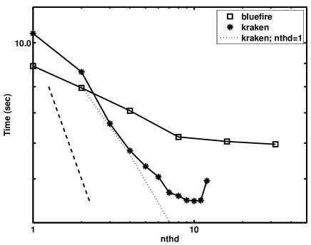
Figure 4: Timing results with a single MPI task and multiple threads on two platforms. Both scale roughly the same for one and 2 threads, but afterward, the bluefire jobs run out–of–socket resulting in poor scaling. The kraken runs scale well up to $7-8$ threads, even though there are only $6$ cores per socket. The dotted line shows the timings for a single thread, while varying the number of MPI processes (hence, the $\mathbf{nthd}$ axis refers to the number of MPI tasks for this curve only). The dashed line represents ideal scaling, and is also used in all subsequent scaling plots.

In the first series of tests, we consider the overhead and performance of OpenMP. The first test thus considers a single MPI process, and variable number of threads nthd with a fixed linear resolution of $N=256$. The results are presented in Fig. 4. The performance for $1$ and $2$ threads is comparable for both platforms. After this, bluefire communicates out–of–socket, and its scaling decreases. We expect that as the core counts increase for this platform (e.g. , as for the Power7 system) this problem will not be as severe. For kraken, there are $6$ cores per socket, but we still see very good scaling to about $7$ threads. Moreover, the departures from the ideal scaling observed in kraken while computing in-socket seem to be associated with the hardware (e.g., with saturation of the memory bandwidth) and not specifically with OpenMP. This we conclude from tests in which OpenMP parallelization is turned off, and the number of MPI tasks is increased. In using from 1 to 6 MPI tasks, the same scaling is observed as with pure OpenMP parallelization (Fig. 4).

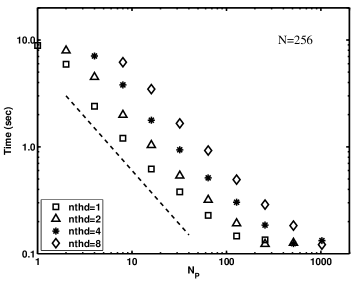
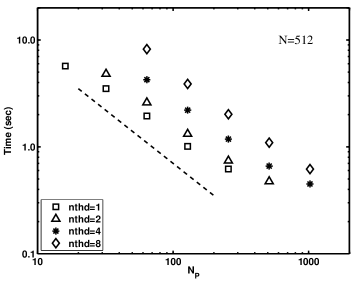
Figure 5: Two sets of bluefire runs, for $N=256$ (left) and for $N=512$ (right). The curves represented by the different symbols are runs at a constant number of threads, as given in the legend. Note, in particular, that the difference in run time between the $1$- and $2$-thread surveys are smaller for the runs with $N=512$, than for the cases where $N=256$, which suggests that the thread overhead will manifest itself with smaller work load on this platform. Also note tje almost linear scalability up to 1000 processors.

In order to examine effects of OpenMP overhead on bluefire results more closely, we compare two runs at different resolutions, one at $N=256$, and one at $N=512$ for a series of thread counts. These results are given in Fig. 5. In each plot the symbols refer to the same $\mathbf{nthd}$, and $N_{P}$ is varied by changing the number of MPI processes. The MPI tasks were bound to processors (using “processor binding”), and symmetric multi-threading (SMT) was disabled. The first observation is that, for $N=256$, the gains as $\mathbf{nthd}$ is increased (for any fixed number of MPI tasks) are roughly the same as the ones reported in Fig. 4 for only 1 MPI task. However, for large numbers of MPI tasks, using $\mathbf{nthd}=2$ gives better timings than $\mathbf{nthd}=1$ using the same total number of processors (e.g., compare the triangle and the square at $N_{P}=256$ with the square at $N_{P}=128$). Increasing the number of threads further does not give substantial speed-ups. This is observed more clearly in the $N=512$ runs. In this case, the slope between runs with $\mathbf{nthd}=1$ and $\mathbf{nthd}=2$ is larger, indicating better gains as the size of the problem is increased.

Table 1: Efficiency of runs with $N$ linear resolution in bluefire, taking as reference runs with $N_{P_{0}}=N/2$ cores and $\mathbf{nthd}=1$ threads.

$N$	$N_{P}=N$, $\mathbf{nthd}=1$	$N_{P}=N$, $\mathbf{nthd}=2$
256	$0.54$	$0.59$
512	$0.58$	$0.65$
1024	$0.63$	$0.66$

As a result, in bluefire there appears to be an effect due to the thread overhead that is noticeable when using 2 threads (in-socket) and the problem size is small: we see that the differences in run time between the $1$-thread and $2$-thread runs is smaller as resolution is increased. Then, as the threads are out-of-socket, extra overhead appears (although for fixed number of threads, very good scaling is found with increasing number of MPI tasks). This can be further observed considering runs with $N=1024$. Table 1 shows the efficiency

$$\epsilon=\frac{N_{P}T}{N_{P_{0}}T_{0}},$$ (3)

where $T$ is the time per time step, and $N_{P_{0}}$ and $T_{0}$ are respectively the number of cores and times measured in a reference run; we consider $N_{P_{0}}=N/2$ with $\mathbf{nthd}=1$ as the reference run. For a fixed number of processors $N_{P}=N$, the efficiency is best if two threads are used instead of one, and as resolution is increased efficiency improves. If $N_{P}=2N$ and four threads are used, efficiency also increases but is at most $\approx 0.4$ for $N=1024$.

These results suggest that a hybrid approach may be most useful for large enough simulations in environments with large processor counts and when a large number of cores is available in the same socket. To verify this we consider the scaling to high core counts on kraken. For these runs, we set $N=1536$, $N=3072$, and $N=4096$, with $\mathbf{nthd}=6\;{\rm or}\;12$. At these resolutions, simulations with 1 thread cannot be executed as there is not enough memory per core in kraken to allocate the arrays. Several simulations at lower resolution ($N=512$) were done to explore configuration parameters. This mainly involved NUMA options in the compiler (PGI), different binding configurations, MPI environment settings, and distribution of jobs among processors. We observed no substantial differences in the timings when changing the job distribution. Binding processors when $\mathbf{nthd}=6$ using the run command instead of NUMA options in the compiler was found to be best, although by a small margin ($\approx 5\%$). The implementation of MPI on kraken can also be configured to do fast copies in memory of the data when sending and receiving large messages. This gives a substantial speed up of the code (8 – $10\%$) but was found to require large amounts of memory that created problems with the largest resolutions. As a result, to compare on an equal footing, the runs described below were compiled with -O2 optimization, without using fast memory copy in MPI, and using the run command

aprun -n $NMPI -S 1 -d $OMP_NUM_THREADS executable

for the $\mathbf{nthd}=6$ runs, and the run command

aprun -n $NMPI -d $OMP_NUM_THREADS executable

for $\mathbf{nthd}=12$. In the former case, the -S 1 option tells aprun to bind one MPI process per socket, and NMPI refers to the total number of MPI processes. It should be noted that in the runs for which the most aggressive optimization options can be used (e.g., if enough memory is available), improvements in the times of up to $20\%$ were found.

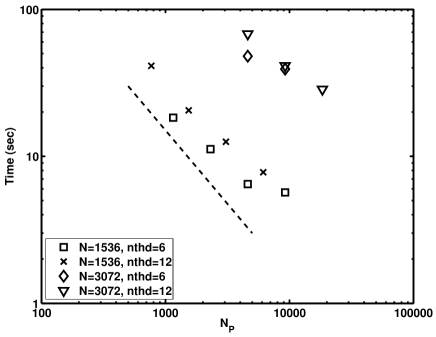
Figure 6: Scalability timings for two sets of runs on kraken. The squares and crosses represent the timings for a $N=1536$ run using $6$ and $12$ threads, respectively. The triangles, and diamonds represent the same for a run size of $N=3072$. Note the cross–over in performance at about $N_{P}=10000$ where the $\mathbf{nthd}=12$ configuration outperforms the $\mathbf{nthd}=6$ configuration for both problem sizes.

The results are given in Fig. 6. We see that good speedup is achieved up to $\sim 20000$ cores, but there are some interesting observations. The mean parallel efficiencies for these runs are $76$, $83$, $61$, and $71\%$, respectively, from top to bottom in the legend of Fig. 6. Maximum efficiencies observed are slightly above 1, indicating super-scaling for some configurations. The efficiency measured for the jobs with larger processor count is given in Table 2. Based on the results shown in Fig. 4, we can expect optimal results for $\mathbf{nthd}=6$. However, the runs with $\mathbf{nthd}=12$ scale uniformly better than the $\mathbf{nthd}=6$ runs. Moreover, from the point of view of actual timings the $\mathbf{nthd}=6$ cases perform better up to a certain point at which the $\mathbf{nthd}=12$ runs outperform them; this point appears to occur at about the same $N_{P}$ for both sets of runs. This is particularly clear for the run with $N=3072$, where the same times are measured for $N_{P}\sim 10000$ using $\mathbf{nthd}=6$ and $\mathbf{nthd}=12$. The results are consistent with the findings in bluefire, but the larger processor count and cores-per-socket in kraken allow us to obtain significant gains using the hybrid approach in the latter case. We conclude that if the workload per MPI process becomes too small, it is better to use more threads even if this puts threads out-of-socket.

Table 2: Efficiency of runs with $N=3072$ linear resolution in kraken, taking as reference runs with $N_{P_{0}}=N_{P}/2$ cores and same number of threads.

$N_{P}=9216$, $\mathbf{nthd}=6$	$N_{P}=9216$, $\mathbf{nthd}=12$	$N_{P}=18432$, $\mathbf{nthd}=12$
$0.58$	$0.61$	$0.72$

5 Discussion and conclusion

We have presented a hybrid MPI-OpenMP model for a pseudo–spectral CFD code. Beginning with an underlying “slab” domain decomposition adequate for parallelization by MPI, we have shown how the basic method is modified by loop–level parallelization to create a two–level parallelization scheme. The new level of parallelization can be thought of as modifying the underlying domain decomposition scheme, and we have pointed out precisely how this has been done depending on the size of the problem, number of threads, and number of MPI tasks.

The hybrid code has been tested primarily on two systems: the IBM Power6 system bluefire at NCAR, and the Cray XT5 system kraken at NICS. We have tested the thread overhead and performance, and found limitations of small socket core counts in bluefire. We have also discovered that there is a resolution threshold, $N$, below which the thread overhead manifests itself more clearly on bluefire and reduces scalability. In terms of large core counts, our results show good scalability up to about $20000$ processors on the kraken system. For large enough problems, we find the best scalability when the number of threads is $12$ (one MPI process per compute node). On the other hand, we find that the performance time is better when $\mathbf{nthd}=6$, until the workload per MPI process is large enough, at which point, the performance time is better for the case where $\mathbf{nthd}=12$. We find that, for a given MPI/OpenMP configuration, and a given resolution, the results are consistent from run–to–run, with little fluctuation in terms of scalability or run time.

Our experimentation has suggested a number of ways in which to improve the compute time of kraken runs. Perhaps the most important of these involve configuring the MPI environment. For the large message sizes we are using, setting the MPI environment variable MPICH_FAST_MEMCPY yields an $8-10\%$ speedup over runs that do not use it, but it requires significantly more buffer memory. This increase in buffer requirements can prevent the code at large resolutions from fitting into memory, and must be considered carefully before attempting a production run. As an example, for $N=4096$ using this configuration, we could only execute the code using 24576 processors and 6 threads, and any other distribution using the same or smaller number of processors and changing the number of threads failed because of insufficient memory. We have not attempted larger resolution runs yet, but we note that the memory issue addressed here will become more of a concern the larger $N$ becomes.

The hybrid scheme introduced here is not the only way in which to decompose the pseudo–spectral grid. An alternative is to retain a pure MPI model as in [15]. In this model, the domain decomposition takes the form of “pencils” which yield a 2D ($N^{2}$) distribution among MPI processes, and OpenMP is not required. This technique is also found to scale well [3] to large core counts, although severe fluctuations in performance are observed even within a given processor–domain mapping. The pure MPI model does not suffer from effects of thread overhead (thread re-starts and synchronization) that we observe in smaller resolution runs, nor from potential problems with compiler optimizations that may arise when OpenMP is used [9]. Nevertheless, the hybrid method described here can be applied to non–Fourier basis spectral methods which may be impossible to parallelize with the 2D distribution (e.g. , spherical harmonics). As pointed out in Section 3, our hybrid method offers a two–level parallelization method that may be more effective in mapping the domain to the hierarchical architectures that are now emerging, and better suited for environments with multiple cores per socket. Indeed, as noted in Section 4, based on our tests on bluefire and kraken we expect the hybrid approach to provide better performance results in coming years, as the number of cores per socket continues to increase. The hybrid scheme may also aid in the MPI memory problems mentioned above, in that fewer MPI processes require less buffer memory. We intend in the future to continue testing this method to higher resolution as accessibility to a larger number of processors becomes more readily available. Since the code described here integrates the Navier-Stokes or magnetohydrodynamics equations when coupling to a magnetic field, including rotation, the hybrid scheme we have developed will prove useful in a variety of geophysical and astrophysical phenomena. And finally, we note that this approach works well even if the aspect ratio of the computational domain is not equal to unity.

References

- [1] C. Canuto, M. Y. Hussaini, A. Quateroni, and T. A. Zang. Spectral Methods in Fluid Dynamics. Springer (New York), 1988.
- [2] P. Dmitruk, L.-P. Wang, W. H. Matthaeus, R. Zhang, and D. Seckel. Scalable parallel FFT for simulations on a Beowulf cluster. Parallel Computing, 27:1921–1936, 2001.
- [3] D. A. Donzis, P. K. Yeung, and D. Pekurovksy. Turbulence simulations at o() core counts. In TeraGrid ’08 Conference, Las Vegas, NV, 2008. Science track paper.
- [4] M. Frigo and S. G. Johnson. The design and implementation of FFTW3. In Proc. IEEE Intl. Conf. Acoustics Speech and Signal Processing, volume 3, page 1381, 1998.
- [5] M. Frigo and S. G. Johnson. The design and implementation of FFTW3. In Proceedings of the IEEE, volume 93, pages 216–231. New York, Academic Press, Inc, 2005.
- [6] D. O. Go’mez, P. D. Mininni, and P. Dmitruk. Parallel simulations in turbulent MHD. Physica Scripta, T116:123–127, 2005.
- [7] D. Gottlieb, M. Y. Hussaini, and S. A. Orszag. Spectral Methods for Partial Differential Equations. SIAM, Philadelphia, 1984.
- [8] D. Gottlieb and S. A. Orszag. Numerical Analysis of Spectral Methods: Theory and Application. SIAM, Philadelphia, 1977.
- [9] G. Hager, G. Jost, and R. Rabenseifner. Communication characteristics and hybrid MPI/OpenMP parallel programming on clusters of multi-core SMP nodes. In Cray User Group Proceedings, 2009. http://www.cug.org/5-publications/proceedings_attendee_lists/CUG09CD/CUG2009/pages/1-program/final_program/20.tuesday.html.
- [10] A. N. Kolmogorov. Dissipation of energy in locally isotropic turbulence. Dokl. Akad. Nauk SSSR, 32:16–18, 1941.
- [11] A. N. Kolmogorov. The local structure of turbulence in incompressible viscous fluid for very large Reynolds number. Dokl. Akad. Nauk SSSR, 30:9–13, 1941.
- [12] S. A. Orszag. Comparison of pseudospectral and spectral approximation. Stud. Appl. Math., 51:253–259, 1972.
- [13] G. Patterson and S. A. Orszag. Spectral calculations of isotropic turbulence: efficient removal of aliasing interactions. Phys. Fluids, 14:2538–2541, 1971.
- [14] D. Takahashi. A hybrid MPI/OpenMP implementation of a parallel 3-D FFT on SMP clusters. In et al. R. Wyrzykowski, editor, Parallel Processing and Appied Mathematics, pages 970–977. Springer Berlin / Heidelberg, 2006. Lecture Notes in Computer Science, vol. 3911.
- [15] P.K. Yeung, D.A. Donzis, and K.R. Sreenivasan. High Reynolds number simulation of turbulent mixing. Phys. Fluids, 17:081703, 2005.
- [16] E. Yilmaz, R.U. Payli, H.U. Akay, and A. Ecer. Hybrid parallelism for CFD simulations: Combining MPI with OpenMP. In I.H. Tuncer, U. Gülcat, D.R. Emerson, and K. Matsuno, editors, Parallel Computational Fluid Dynamics, volume 67, pages 401–408. Springer Berlin Heidelberg, 2007. Lecture Notes in Computational Science and Engineering.