Octupole deformation properties of the Barcelona Catania Paris energy density functionals

Abstract

We discuss the octupole deformation properties of the recently proposed Barcelona-Catania-Paris (BCP) energy density functionals for two set of isotopes, those of radium and barium, where it is believed that octupole deformation plays a role in the description of the ground state. The analysis is carried out in the mean field framework (Hartree- Fock- Bogoliubov approximation) by using the axially symmetric octupole moment as a constraint. The main ingredients entering the octupole collective Hamiltonian are evaluated and the lowest lying octupole eigenstates are obtained. In this way we restore, in an approximate way, the parity symmetry spontaneously broken by the mean field and also incorporate octupole fluctuations around the ground state solution. For each isotope the energy of the lowest lying $1^{-}$state and the $B(E1)$ and $B(E3)$ transition probabilities have been computed and compared to both the experimental data and the results obtained in the same framework with the Gogny D1S interaction, which are used here as a well established benchmark. Finally, the octupolarity of the configurations involved in the way down to fission of ²⁴⁰Pu, which is strongly connected to the asymmetric fragment mass distribution, is studied. We confirm with this thorough study the suitability of the BCP functionals to describe octupole related phenomena.

I Introduction

The ground state and low lying excited states of many atomic nuclei all over the nuclide chart show quadrupole deformation in their intrinsic states Bohr.75 . This property has profound consequences in the low lying spectrum of those nuclei as well as in their decay patterns Ring.80 ; Bender.03 . Octupole deformation is not as common as quadrupole deformation as a characteristic of the ground state of atomic nuclei, but its consequences are important for understanding nuclear properties of several actinide nuclei around radium and several rare earth around barium Butler.96 . The octupole operator has negative parity and therefore a non-zero octupole deformation means that the intrinsic state has lost reflection symmetry and acquired a pear-like shape. The quantum interference between the two degenerate intrinsic states with pear-shaped matter distributions pointing upward and downward (i.e. with the same absolute value of the octupole moment but opposite sign) restores the parity quantum number and leads to the presence in the spectrum of a doublet with opposite parities Bohr.75 ; Butler.96 . The energy splitting between the two members of the doublet strongly depends upon the properties of the barrier separating the two degenerate intrinsic states with opposite octupole moment. In deformed even-even nuclei it is possible that the negative parity member of the ground state multiplet , the lowest lying $1^{-}$ state, can be located below the lowest $2^{+}$state leading to the appearance of alternating parity rotational bands, which are clear signatures of octupole deformation. Also, the two members of the doublet will be connected by strong $B(E1,1^{-}\rightarrow 0^{+})$ transition probabilities from the $1^{-}$ to the ground state. The next member of the negative parity rotational band is a $3^{-}$ that rapidly decays to the $0^{+}$ground state by means of strong $B(E3,3^{-}\rightarrow 0^{+})$ transition probabilities. Although there are several known examples of alternating parity rotational bands at low spins, the alternating behavior usually appears at high spins as a consequence of the stabilizing effect of angular momentum on the octupolarity of the system: moments of inertia increase with the octupole moment and therefore configurations with higher octupole moments are the more lowered by increasing angular momentum.

The appearance of octupole effects is strongly linked to the position of the Fermi energy in the single particle spectrum of the underlying mean field Bohr.75 ; Butler.96 . The reason is that octupolarity is enhanced when, in a given major shell, the intruder orbital interacts (via a particle-hole excitation) with a nearby normal parity orbital with three units less of angular momentum ($3\hbar$ is the amount of angular momentum carried out by the octupole operator). This happens between the $j_{15/2}$ and $g_{9/2}$ spherical orbitals, the $i_{13/2}$ and $f_{7/2}$ and the $h_{11/2}$ and $d_{5/2}$. Those regions where both protons and neutrons feel a strong octupole interaction is where octupole related effects are expected to be more pronounced. For example, in the region around ${}_{88}^{224}$Ra, the Fermi level of protons is located around the $f_{7/2}$orbital that can then interact strongly with the empty $i_{13/2}$. Besides, Fermi level of neutrons is around the $g_{9/2}$ orbital, which strongly interacts through the octupole interaction with the $j_{15/2}$ one. Similar arguments apply to the region around ¹⁴⁴Ba with the orbitals $d_{5/2}$ and $h_{11/2}$ for protons and the $f_{7/2}$ and $i_{13/2}$ for neutrons responsible for octupolar effects.

Last but not least, octupolarity also plays a relevant role in the asymmetric fission decay mode because an octupole deformed pathway to fission naturally explain the observed asymmetric mass fragment distribution of several actinide parent nuclei Fission .

In this article we want to check the ability of the recently proposed Barcelona-Catania-Paris (BCP) energy density functionals Baldo.08 , in dealing with the octupole degree of freedom in finite nuclei. We will compare the results provided by the BCP functionals in some test cases with experimental values, when available, and with the results obtained using the Gogny D1S interaction that we take here as a benchmark. The BCP energy density functionals consist of a bulk part which is fully microscopic and comes from the nuclear and neutron equation of state Baldo.04 which are parametrized in a polynomial form complemented by additional terms accounting for finite size effects (see Fayans.98 ; Fayans.01 for functionals inspired in the same principles). In addition to the Coulomb term and the spin-orbit contribution, which is taken exactly as in the Skyrme or Gogny forces, we add a purely phenomenological finite range term for describing properly the nuclear surface. To deal with open-shell nuclei we still include in the BCP functionals a zero range density-dependent pairing interaction fitted to reproduce the nuclear matter gaps obtained with the Gogny force Garrido.99 . The only free parameters of these functionals are the isospin like (L) and unlike (U) strengths of the surface term, the range of the Gaussian form factor used to give a finite range to the surface term and the strength of the spin-orbit interaction Baldo.08 . These free parameters are adjusted in the usual way to reproduce the ground state energy and charge radii of some selected spherical nuclei. With these ingredients, the BCP functionals give an excellent description of 161 even-even spherical nuclei with rms values for the ground-state energies (1.77 MeV and 2.06 MeV) for BCP1 and BCP2, respectively) and charge radii that are comparable to the ones obtained with well reputed interactions/functionals like Skyrme SLy4 (1.71 MeV), Gogny D1S (2.41 MeV) or the Relativistic NL3 parametrization (3.58 MeV). Apart from the advantages already mentioned in Baldo.08 , the BCP functionals are advantageous in its application to finite nuclei because of its reduced computational cost as compared to Gogny (BCP is a factor between 6 to 10 faster) or even Skyrme (comparable computational cost). Also the appearance of integer powers of the density in the bulk part of the functional, which is a consequence of the specific fit to the nuclear matter results, makes much easier to deal with the self-energy problem that plagues beyond mean field calculation Duguet.09 . Using these BCP functionals we have also explored quadrupole deformation properties robledo.08 . We find a behavior similar to that obtained using the Gogny D1S force widely used to this end. This fact give us confidence in using the BCP functionals to study nuclear properties related to deformation. As the BCP functionals are aimed at describing not only masses and radii but also the low lying spectrum over all the nuclide chart, it is necessary to check whether the very reasonable results regarding quadrupole collectivity can also be extended to the octupole deformation case. To check that this is the case, we have carried out mean field Hartree- Fock- Bogoliubov (HFB) calculations with the BCP energy density functional as well as the Gogny Decharge.80 D1S Berger.84 interaction to test the response of the system to the octupole degree of freedom. To be more precise, we have used a constraint in the axially symmetric octupole moment to generate potential energy curves (PECs) to search for octupole deformed minima as well as to study the stiffness of those (and other) minima against changes in the octupole degree of freedom. These PECs are computed for several isotopes of radium from ²¹⁶Ra to ²³²Ra and of barium from ¹⁴⁰Ba until ¹⁵⁰Ba. In addition to the PEC, the calculation of the corresponding collective inertias allows the evaluation of the $1^{-}$ excitation energy as well as $B(E1)$ and $B(E3)$ transition probabilities in the framework of the collective Schrödinger equation (CSE) method. The results will be compared with experimental data, when available, as well as with the results obtained with the Gogny D1S force. It should be mentioned that the Gogny D1S results have already been reported in Refs. Robledo.87 ; Egido.89 ; Egido.90 and similar calculations with the Skyrme interactions exist in the literature Bonche.86 . Finally, the octupole properties of the fission valley of ²⁴⁰Pu will also be briefly discussed and compared to those of Gogny D1S.

II Theoretical tools

To solve the Hartree-Fock-Bogoliubov (HFB) equation Ring.80 the quasi-particle operators of the Bogoliubov transformation have been expanded in a harmonic oscillator (HO) basis big enough as to warrant convergence of the results with the basis size. The expansion coefficients have been determined by means of the gradient method which relies on the parametrization of the mean field (HFB) energy in terms of the parameters of the Thouless expansion of the most general HFB wave functions. Within the gradient method, the HFB problem is recast in terms of a minimization (variational) process of the mean field energy and the search of the minimum is performed by following the direction of the gradient in the multidimensional space of parameters. The advantage of this method over the more traditional one of successive diagonalizations is in the way the constraints are implemented, which allows a larger number of them to be treated at once. Axial symmetry has been preserved in the calculation implying the use of an axially symmetric HO basis made up of the tensor product of two dimensional HO wave functions times one dimensional HO ones. Along with the octupole moment constraint associated to the multipole operator $\hat{Q}_{3}=r^{3}Y_{30}$ and used to generate the PEC’s, we have included a constraint on the center of mass of the nucleus (i.e. the mean value of $r^{1}Y_{10}$ has been set to zero) to prevent spuriousness associated to the center of mass motion, to slip into the results. As a consequence of the axial symmetry imposed in the HFB wave functions, the mean values of the $Q_{\lambda\mu}$ multipole operators with $\mu\neq 0$ are zero by construction.

The information given by mean field theories is restricted to the energy and shape of the -generally- deformed ground state. To restore the parity symmetry broken by the mean field approximation and to describe the dynamics of the collective excited states it is mandatory to go beyond the mean field approximation. With this in mind, the octupole degree of freedom $Q_{3}=\langle\psi|\hat{Q}_{3}|\psi\rangle$ (where $|\psi\rangle$ is the HFB intrinsic wave function) has been used to build up a collective Hamiltonian based on the Generator Coordinate Method (GCM) and the Gaussian Overlap Approximation (GOA) Brink.68 ; Giraud.74 ; Reinhard.87 . In this method, the GOA is used to reduce the Hill-Wheeler equation of the GCM to a Schrödinger equation for the collective wave function, the so-called Collective Schrödinger Equation (CSE)

$$\hat{{\cal\mathcal{H}}}_{coll}\phi_{\alpha}(Q_{3})=\epsilon_{\alpha}\phi_{\alpha}(Q_{3}),$$ (1)

where the collective Hamiltonian $\hat{{\cal H}}_{coll}$ is given by

$$\hat{{\cal\mathcal{H}}}_{coll} = -\frac{1}{\sqrt{G(Q_{3})}}\frac{\partial}{\partial Q_{3}}\sqrt{G(Q_{3})}\frac{1}{2B(Q_{3})}\frac{\partial}{\partial Q_{3}}$$ (2)

$$+ V(Q_{3})-\epsilon_{0}(Q_{3}).$$ (3)

In this expression $G(Q_{3})$ is the metric, $B(Q_{3})$ is the mass parameter associated with the collective motion along $Q_{3}$, $V(Q_{3})$ is the collective potential given by the HFB energy $V(Q_{3})=\langle\psi(Q_{3})|\hat{H}|\psi(Q_{3})\rangle$ and $\epsilon_{0}(Q_{3})$ is the Zero Point Energy (ZPE) correction. The eigenfunctions $\phi_{\alpha}(Q_{3})$ of Eq. (1) have to be normalized to one with the metric $G(Q_{3})$

$$\int dQ_{3}\,\sqrt{G(Q_{3})}\,\phi_{\alpha}^{*}(Q_{3})\phi_{\beta}(Q_{3})=\delta_{\alpha,\beta}$$ (4)

to preserve the hermiticity of $\hat{{\cal\mathcal{H}}}_{coll}$.

It should be mentioned that a CSE can also be obtained from the Adiabatic Time Dependent Hartree- Fock (ATDHF) theory Baranger.78 ; Brink.76 ; Villars.77 after quantization of the semi-classical Hamiltonian for the slow moving collective degrees of freedom. The collective Hamiltonian obtained in this way has the same functional form as the GCM+GOA one, but the expression of the collective parameters is different. Later we will discuss how to choose these collective parameters.

An interesting characteristic of the collective Hamiltonian for the octupole degree of freedom is that $\hat{{\cal H}}_{coll}$ is invariant under the exchange $Q_{3}\rightarrow-Q_{3}$ and, therefore, it is possible to classify its eigenfunctions, $\phi_{\alpha}(Q_{3})$, according to their parity under the $Q_{3}\rightarrow-Q_{3}$ exchange. It is easy to see that the parity of the collective wave function under the $Q_{3}\rightarrow-Q_{3}$ exchange corresponds to the spatial parity operation in the correlated wave function built up from $\phi_{\alpha}$. The inclusion of octupole correlations immediately restores the parity symmetry lost at the mean field level. Therefore, the solution of the CSE Eq. (1) allows the calculation of the $0^{+}-1^{-}(3^{-})$ energy splitting and the B(E1) and B(E3) transition probabilities connecting them. At this point it has to be pointed out that in the present framework where only time reversal invariant wave functions are considered it is only possible to describe excited states with average angular momentum zero. To deal with genuine $1^{-}$ or $3^{-}$states cranking model wave functions should be considered, which is out of the scope of the present work. Here we will assume that the cranking rotational energy of the $1^{-}$state is much smaller than the excitation energy of the negative parity band head and therefore can be safely neglected. Also the impact of the cranking term in the transition probabilities to be discussed next is neglected. With these approximation in mind, the reduced transition probabilities from the lowest $1^{-}$ and $3^{-}$ states to the $0^{+}$ ground state can be computed within the Rotational Model approximation as

$$B(E\lambda,I_{f}\rightarrow I_{i})=e^{2}\langle I_{i}K\lambda 0|I_{f}K\rangle^{2}|\langle\varphi_{i}|r^{\lambda}Y_{\lambda,0}|\varphi_{f}\rangle|^{2},$$ (5)

where $|\varphi_{i}\rangle$ and $|\varphi_{f}\rangle$ are correlated wave functions obtained in the spirit of the GCM from the collective wave functions $\phi_{\alpha}(Q_{3})$. The preceding formula can be reduced to an expression involving those collective wave functions $\phi_{\alpha}(Q_{3})$ by means of the GOA Nerlo.87 . The final result for $K=0$ bands reads

$$B(E1,1^{-}\rightarrow 0^{+})=\frac{e^{2}}{4\pi}\left|\langle\phi_{0^{-}}|D_{0}|\phi_{0^{+}}\rangle_{\textrm{COLL}}\right|^{2}$$ (6)

for the E1 electric transition and

$$B(E3,3^{-}\rightarrow 0^{+})=\frac{e^{2}}{4\pi}\left|\langle\phi_{0^{-}}|Q_{30}(\textrm{PROT)}|\phi_{0^{+}}\rangle_{\textrm{COLL}}\right|^{2},$$ (7)

for the E3 one. In the preceding formulas we have introduced the collective matrix element of an operator $\hat{O}$ as

$$\langle\phi_{0^{-}}|\hat{O}|\phi_{0^{+}}\rangle_{\textrm{COLL}}=\int dQ_{3}\,G^{1/2}\,\phi_{0^{-}}^{*}(Q_{3})O(Q_{3})\phi_{0^{+}}(Q_{3})$$

where $O(Q_{3})=\langle\psi(Q_{3})|\hat{O}|\psi(Q_{3})\rangle$. In Eq. (6) $D_{0}$ is the dipole moment operator whose mean value is defined as the difference between the center of mass of protons and neutrons

$$D_{0}(Q_{3})=\frac{N}{A}\langle\psi(Q_{3})|\hat{z}_{prot}|\psi(Q_{3})\rangle-\frac{Z}{A}\langle\psi(Q_{3})|\hat{z}_{neut}|\psi(Q_{3})\rangle.$$ (8)

Finally, $Q_{30}(\textrm{PROT)}$ is the part of the octupole operator acting on proton’s space.

To carry out the collective calculations it is necessary to specify the collective parameters $G(Q_{3})$, $B(Q_{3})$ and $\epsilon_{0}(Q_{3})$ appearing in the definition of $\hat{\mathcal{H}}_{coll}$ Eq. (2). As it was said before, there are two sets of parameters coming from the GCM+GOA and the ATDHF derivation of the collective Hamiltonian. The set of parameters used in this calculation is an admixture of the two and it is known as the ATDHF+ZPE set. It includes the mass parameter $B(Q_{3})$ coming out from the semi-classical Hamiltonian of the ATDHF theory, the metric of the GCM+GOA and the ZPE correction computed with the GCM+GOA formula but using the ATDHF mass instead, i.e.

$$\epsilon_{0}(Q_{3})=\frac{1}{2}G(Q_{3})B(Q_{3})_{ATDHF}^{-1}.$$ (9)

This set of parameters was devised to put together the advantages of the ATDHF set (time-odd components included in the mass term) and the ones of the GCM+GOA (ZPE correction). This method can be somewhat justified in the context of the extended GCM Reinhard.87 ; Villars.75 and has been extensively used Berger.84 ; Egido.89 .

The calculation of the collective parameters involves the inversion of the HFB stability matrix which is closely related to the matrix of the RPA equation. At present, this is a formidable task and approximations are needed. The approximation used in this article – called “cranking approximation" Reinhard.78 ; Girod.79 – neglects the off-diagonal terms of the stability matrix allowing to invert it analytically but at the cost of including the two body interaction only through the mean field. Although this approximation has been extensively used in the literature for the calculation of collective masses and moments of inertia (see, for instance, Refs. Baran.81 ; Berger.84 ; Boning.85 ) its validity has not been properly established. Using the “cranking approximation”, the ATDHF+ZPE parameters are given by

$$G(Q_{3})=\frac{M_{-2}(Q_{3})}{2M_{-1}^{2}(Q_{3})},\,\,\,B(Q_{3})=\frac{M_{-3}(Q_{3})}{M_{-1}^{2}(Q_{3})};$$ (10)

where the quantities $M_{-n}(Q_{3})$ ($n=1,2,3$ ) are defined as

$$M_{-n}(Q_{3})=\sum_{k,l}\frac{\left|\left(Q_{30}\right)_{kl}^{20}\right|^{2}}{(E_{k}+E_{l})^{n}}.$$ (11)

In the preceding expression, $E_{k}$ are the quasi-particle energies and $\left(Q_{30}\right)_{kl}^{20}$ are the matrix elements of the $20$ part Ring.80 of the octupole operator $\hat{Q}_{30}$ in the quasi-particle basis of the HFB wave function $|\psi(Q_{3})\rangle$. This form of the collective mass is usually referred to in the literature as Belyaev-Inglis mass Ring.80 .

III Results

In the subsequent subsections the results obtained with the BCP1 Baldo.08 functional and regarding octupole properties of some radium and barium isotopes will be discussed. The other functional defined in Baldo.08 and referred to as BCP2 will not be explicitly considered here although the calculations were carried out for that case too. The reason is the strong similarities between BCP1 and BCP2 results that produced most of the curves one on top of another, making it impossible to differenciate them in the plots presented.

III.1 Low excitation energy properties in the radium isotopes

Octupole deformation properties of the radium isotopes were the first to be addressed from a microscopic point of view with the Gogny force, first at the mean field level Egido.89 and next including exact restoration of the parity symmetry Egido.91 . At the mean field level, the first quantity to analyze is the potential energy curve (PEC) as a function of the octupole moment that determines both the ground state minimum and its stiffness. Let us point out that for every point in the PEC the other multipole moments (quadrupole, hexadecapole, etc) are selfconsistently determined as to produce the lowest energy. The PECs computed with the BCP1 Baldo.08 energy density functional and the Gogny D1S Decharge.80 ; Berger.84 force are depicted in Fig. 1. As can be seen in the plot, the results for the two types of interactions look very similar in all the nuclei considered. It is observed how, whenever a minimum appears (in the nuclei from ²¹⁸Ra to ²²⁸Ra) in the Gogny D1S calculation at an octupole deformation different from zero, the same happens and at the same $Q_{3}$ value in the BCP1 calculation. For the nuclei with the minimum at $Q_{3}=0$ the Gogny D1S force shows a tendency to produce a stiffer parabolic behavior in the PEC than in BCP1. The depth of the octupole deformed minima is also very similar for both kinds of calculations and reaches its maximum value of 1.5 MeV for the nucleus ²²²Ra which therefore can be considered as the strongest octupole deformed nuclei of the considered chain.

Figure 1: The HFB mean field energy as a function of the octupole moment $Q_{3}$ (in units of $b^{3/2}=10^{3}\textrm{ fm}^{3}$) for the isotopes of radium (Z=88) from A=216 up to A=232. Results for both the BCP1 energy density functional (full curves) and the Gogny D1S force (dotted curves) are shown.

Figure 2: The particle-particle (pp) correlation energy defined as $E_{pp}=\frac{1}{2}\textrm{Tr}\Delta\kappa$ is plotted as a function of the octupole moment $Q_{3}$ (in units of $b^{3/2}=10^{3}\textrm{ fm}^{3}$) for the radium isotopes considered. Dotted lines correspond to the pp correlation energies whereas full lines are meant to represent the same quantity for protons. Thick lines are used to depict the results of the calculations with the BCP1 functional whereas thin lines are for the results with the Gogny D1S force.

In Fig 2 we show the particle-particle correlation energy defined as $E_{pp}=\frac{1}{2}\textrm{Tr}\Delta\kappa$ and given in terms of the usual pairing field $\Delta$ and pairing tensor $\kappa$ of the HFB method. This quantity gives a rough idea of the amount of pairing correlations in the system. It can also be used as an indicator of the size of the single particle level density around the Fermi surface as strong pairing correlations are direct consequence of high level densities. This energy is also correlated with the pairing gap that represents the energy of the lowest two quasi-particle excitation and therefore it is closely related to the collective inertias to be discussed below. The overall tendency of $E_{pp}$ is to decrease with increasing octupole moment up to values of $Q_{3}=10$ b^3/2which correspond to typical excitation energies of 5-6 MeV above the ground state in the PECs. From there on we observe, depending on the nucleus, stationary behaviors or mild increases. We also notice that the $E_{pp}$ computed with BCP1 are greater than the ones computed with D1S for the light isotopes ²¹⁶Ra and ²¹⁸Ra and for the two species of nucleons. For the nucleus ²²⁰Ra the particle-particle correlation energies for protons and neutrons are similar in both calculations and from there on and up to the ²³⁰Ra isotope the D1S correlation energies are larger than the BCP1 ones. For the heaviest isotope considered ²³²Ra the $E_{pp}$ energy for neutrons is larger for BCP1 than for D1S and the opposite is true for protons.

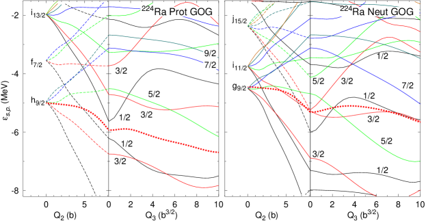
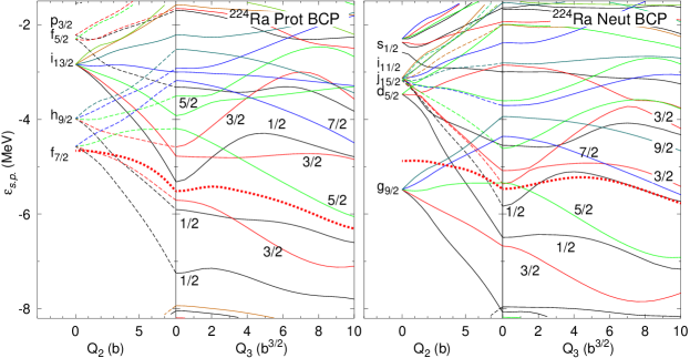
Figure 3: (Color online) Single particle energies (SPE) of the nucleus ²²⁴Ra both for protons (left panels) and neutrons (right panels) and the two interactions/functionals used in the calculations (Gogny D1S in the upper panels, BCP1 in the lower ones). In each panel, the single particle energies are plotted first as a function of the mass quadrupole moment $Q_{2}$ starting at sphericity ($Q_{2}=0$ b) up to the value corresponding to the self-consistent minimum in the quadrupole variable at $Q_{3}=0$ b^3/2 ($Q_{2}$=8.12 b for the Gogny calculation and 7.88 b for the BCP1 one). In this plot the spherical quantum numbers obtained at $Q_{2}=0$ b are given. On the right hand side of each panel, the SPE as a function of the octupole moment starting at $Q_{3}=0$ b^3/2are plotted. The octupole deformed self-consistent minimum is locate in this nucleus at around $Q_{3}=4$ b^3/2. Thick dotted lines indicate the Fermi level. As a consequence of axial symmetry, the $K$ quantum number of each level remains fixed along the plot. Each $K$ value has an associated color (black, $K=1/2$; red, $K=3/2$ ; green, $K=5/2$; blue, $K=7/2$; dark green, $K=9/2$, etc). The parity of each state when $Q_{3}=0$ (i.e., in the $Q_{2}$ plot) is determined by the kind of line: full for positive parity and dashed for negative parity. Finally, the $K$ quantum numbers of specific levels around the Fermi level are given.

In Fig. 3 the single particle energies (SPE) are plotted as a function of the octupole moment $Q_{3}$ for both protons and neutrons. Results of both calculations are shown in different panels ( Gogny D1S upper and BCP1 lower panels). In all the cases, the Fermi level is represented by a thick dotted line. Once the stretching effect of the bigger effective mass of BCP1 (1, versus 0.7 in Gogny D1S) is accounted for, the similitude between the single particle energies obtained with Gogny D1S and BCP1 around the Fermi level and $Q_{3}$ values in the neighborhood of the mean field minimum is remarkable. It is also possible to say that the behavior of most of the levels as a function of both $Q_{2}$ and $Q_{3}$ is quite similar in both kinds of calculations. This is so in spite of the different ordering of the spherical orbitals: for protons the $f_{7/2}$ and $h_{9/2}$ are reversed in the spectrum of Gogny D1S as compared to the spectrum of BCP1. For neutrons there is also such an inversion between the $j_{15/2}$ orbital and the $i_{11/2}$ orbital and also the separation between the $i_{11/2}$ and $g_{9/2}$ orbitals is much larger in BCP1 than in Gogny D1S. That the single particle spectrum looks similar in the region of well developed quadrupole deformation and also as a function of octupole deformation is probably a consequence of the collective character of those collective degrees of freedom where the geometry of the shape of the nucleus is more important than quantum mechanical effects. To make the argument more quantitative, we have analyzed the structure of the single particle wave functions in terms of Nilsson quantum numbers and found that the levels around the Fermi surface have similar structures. A typical example for protons is the $K=5/2^{-}$ level that for $Q_{3}=0$ lies at -4.5 MeV in the D1S case and at -4.2 MeV in the BCP one. This level originates in the $h_{9/2}$ spherical orbital in the D1S case whereas it comes from a $f_{7/2}$ in the BCP one. The Nilsson quantum numbers for the D1S orbital are $[523]$ (66$\%$), $[532]$ (11$\%$), $[503]$ (7$\%$), $[743]$ (6$\%$), and other small components whereas for BCP1 they are $[523]$ (46$\%$), $[532]$ (15$\%$), $[503]$ (9$\%$), $[312]$ (7$\%$) and smaller components. We can also consider another example in the neutron side where, at $Q_{3}=0$ there is a $K=3/2^{+}$ orbital at around -5 MeV that originates from a $i_{13/2}$ spherical level in the D1S calculations and from a $d_{5/2}$ in the BCP one. The Nilsson quantum numbers obtained are $[631]$ (31$\%$), $[642]$ (25$\%$), $[611]$ (15$\%$), $[862]$ (8$\%$) and small components for D1S and $[642]$ (47$\%$), $[631]$ (16$\%$), $[862]$ (13$\%$), $[422]$ (7$\%$) and small components for BCP. From the preceding examples and other orbitals considered (but not displayed here) we conclude that the quantitative structure of the levels is quite similar in the two calculations irrespective of their spherical origin. This reinforces our suggestion about the fundamental role played by the collective degrees of freedom in the determination of single particle wave functions.

The conditions for the development of octupolarity are clearly satisfied in this nucleus as can be seen in the single particle plot: for protons there are “$f_{7/2}$” levels below the Fermi level with $K=1/2$ and 3/2 and at the same time $i_{13/2}$ orbitals with $K=1/2$ and $3/2$ are just above the Fermi level. The same happens in the neutron case with the $g_{9/2}$ orbital well below the Fermi level and the $j_{15/2}$ with $K=1/2$ and 3/2 at the Fermi level (please remember the super-fluid character of neutrons that makes the Fermi level concept a diffuse one). Another condition for the development of a minimum is the presence of a region of low level density in the SPE spectrum (Jahn-Teller effect, see Ref. Bohr.75 for a general discussion in the nuclear context). We observe in the two proton spectra in Fig. 3 how the Fermi level of protons lies in the middle of a low level density region at $Q_{3}=4$ b^3/2 which corresponds to the position of the minimum. For neutrons and around $Q_{3}=4$b^3/2 we also observe a region of low level density near the Fermi level which is more pronounced for the BCP1 results. As the number of neutrons is increased the Fermi level moves upward and enters a region of high level density that is unable to lead to a deformed minimum as is the case for ²³⁰Ra and heavier isotopes.

Finally, we would like to mention that the differences observed in the position of the single particle levels in Fig. 3 has little impact on the quantum numbers of neighboring odd-A nuclei as in the present mean field framework those quantum numbers have to be obtained after a selfconsistent blocking mean field procedure and it is not enough to block the single particle orbitals of Fig. 3 as would be the case with a description based on a Nilsson diagram. Work to implement such blocking mechanism in the BCP case is under way and will be reported in the near future.

In Fig. 4 we show the collective inertia $B(Q_{3})$ associated with the octupole degree of freedom (see Eqs. (10) and (11)) and playing a central role in the collective Schrödinger Hamiltonian of the previous section. As a consequence of the presence in its definition of a denominator with powers of the two quasiparticle energies $E_{\mu}+E_{\nu}$, the collective inertia is roughly speaking inversely proportional to the amount of pairing correlations (the pairing gap to be more quantitative) and directly proportional to the effective mass of the interaction. The lower pairing correlations present in BCP1 are not able to compensate for the higher effective mass and as a consequence the BCP1 inertias are higher than the Gogny D1S ones. Thus the energies obtained as a solution of the one dimensional collective Hamiltonian, which are roughly speaking proportional to the inverse of the square root of the collective mass (remember the standard harmonic oscillator formula relating the oscillator’s frequency $\omega$ with the spring constant and the mass $\omega=\sqrt{k/m}$), are expected to reach lower values for BCP1 than for D1S. It is also worth noticing that the peaks observed in the $B(Q_{3})$ plots are related to regions of low pairing correlations as is easily deduced by comparing Fig. 4 with Fig. 2.

Figure 4: The octupole collective inertia parameter $B(Q_{3})$ entering the one dimensional collective Schrödinger Hamiltonian (see text for details) is shown as a function of the octupole moment $Q_{3}$ (in units of $b^{3/2}=10^{3}\textrm{ fm}^{3}$) for the radium isotopes considered. Full lines are for the calculations with the BCP1 functional and dashed ones for the results obtained with the Gogny D1S force.

In Fig 5 the zero point energy correction $\epsilon(Q_{3})$ of Eq. 9 is given for the isotopes of radium considered and the BCP1 functional and the Gogny D1S force. The values of $\epsilon(Q_{3})$ are correlated with the inverse of the collective inertia $B(Q_{3})$, as can easily be noticed by comparing Figs 4 and 5. The range of variation is typically of around half an MeV in the interval of interest between $Q_{3}=0$b^3/2 and $Q_{3}\approx 5$b^3/2 and most of the nuclei considered although there are exceptions like the nucleus ²¹⁶Ra. The effect of the ZPE is to increase the depth of the octupole well for the lighter nuclei ^216-220Ra whereas it is the opposite in all the heavier isotopes. The impact of this effect on the properties of the solutions of the CSE is not as pronounced as it could be thought because of the effect of the collective masses (correlated to the behavior of the ZPE) that tends to cancel out the one of the ZPE.

Figure 5: The octupole zero point energy correction $\epsilon(Q_{3})$ of Eq. 9 is plotted as a function of the octupole moment $Q_{3}$ (in units of $b^{3/2}=10^{3}\textrm{ fm}^{3}$) for the isotopes of radium considered. Full lines are for the calculations with the BCP1 functional and dashed ones for the results obtained with the Gogny D1S force.

Figure 6: The relevant quantities entering the Collective Schrödinger equation for the two cases considered, namely the calculation with the Gogny D1S force (right hand side panels) and the calculation with the BCP1 energy density functional (left hand side panels). In the upper panels, the octupole collective mass $B(Q_{3})$ (already shown in Fig. 4) is depicted as a function of the octupole moment $Q_{3}$ (in units of $b^{3/2}=10^{3}\textrm{ fm}^{3}$). In the lower panels, the thick lines represent the HFB energy (dashed line) and the CSE potential energy (HFB energy minus zero point energy, full line). The thin lines correspond to the square of the collective wave functions corresponding to the lowest positive parity state $|\phi_{0^{+}}(Q_{3})|^{2}$ (full line) and lowest energy negative parity state $|\phi_{0^{-}}(Q_{3})|^{2}$ (dashed line).

Figure 7: In the left hand side panel, the energies of the $1^{-}$states, obtained by solving the 1D collective Schrödinger Hamiltonian, are displayed as a function of the mass number for the radium isotopes considered. Theoretical results (lines, full for the results obtained with the BCP1 functional and dotted for the results obtained with the D1S force) are plotted along with the experimental data (boxes). In the middle panel the $B(E1,1^{-}\rightarrow 0^{+})$ transition probabilities in W.u. are given as a function of the mass number for the radium isotopes considered. Finally, in the right hand side panel the $B(E3,3^{-}\rightarrow 0)$ in W.u. is given for the different radium isotopes considered.

Figure 8: Dipole moments $D_{0}$(fm) are represented as a function of the octupole moment $Q_{3}$ (in units of $b^{3/2}=10^{3}\textrm{ fm}^{3}$) for the nine isotopes of Ra considered. Dashed lines correspond to the results obtained with the Gogny D1S force whereas the full line ones are for the results obtained with the BCP1 functional.

With the potential energy curve, the collective mass and the zero point energy correction, all the ingredients needed to solve the CSE are at our disposal. In Fig. 6 we have shown all those ingredients together in two plots corresponding to the results with the Gogny D1S force and BCP1 functional. In each of the plots we have depicted in the lower panel the HFB energy curve (dashed line) as a function of the octupole moment $Q_{3}$ and shifted to put the minimum at zero energy. The full curve closely following the dotted one is the potential energy entering the CSE that is obtained by subtracting the ZPE energy correction to the HFB energy. As observed in the plot the collective potential energy is rather similar to the HFB energy. Also the HFB energies obtained with the D1S force and the BCP1 functional calculations are rather similar. In the same panel, the square of the collective amplitudes $|\phi_{\alpha}(Q_{3})|^{2}$ for the lowest lying state of each parity are plotted. The negative parity amplitudes look rather similar in both calculations but this is not the case for the positive parity amplitude which is higher around $Q_{3}=0$ for Gogny D1S than for BCP1. The different behavior of the positive parity amplitude is related to the different collective masses obtained in both calculations and given in the upper panels. The Gogny D1S collective mass is much lower around $Q_{3}=0$ than the one obtained with BCP1 and, as discussed in Ref. Egido.89 ; Egido.90 , this enhances the collective amplitude around that value. As a consequence of the lower mass obtained with the D1S force the energy of the $1^{-}$state computed after solving the CSE is higher (200 keV) than the one obtained with the BCP1 functional (73 keV). On the other hand, the effect on the $B(E1,1^{-}\rightarrow 0^{+})$ and $B(E3,3^{-}\rightarrow 0^{+})$ transition probabilities is to yield smaller values for D1S than for BCP1 as the overlap between the positive and negative parity amplitudes is smaller in the later case. However, recalling the expression of the transition probabilities of Eqs. (6) and (7), it is easy to realize the reduced impact of the region around $Q_{3}=0$b^3/2 on the final quantities as each of the factors of the integrands, $D_{0}(Q_{3})$ and $\left(Q_{3}\right)_{prot}(Q_{3})$, are zero for $Q_{3}=0$ b^3/2.

The energies of the $1^{-}$ states and transition probabilities obtained by solving the CSE with the collective parameters deduced from the Gogny D1S and BCP1 calculations are depicted in Fig. 7 along with available experimental values. For the energy of the $1^{-}$ states we observe that both the BCP1 functional and the Gogny D1S interaction reproduce quite nicely the experimental isotopic trend (see Butler.91 ; Butler.96 and references therein) with a minimum around A=224. The very good reproduction of the experimental data in the calculation with Gogny D1S can be considered as accidental in the sense that the absolute values of the $1^{-}$excitation energies crucially depend on the amount of pairing correlations (through the collective mass) which are not so well characterized at the mean field level. A more robust indicator of the quality of the results is the reproduction of the isotopic trend which is very good in both, D1S and BCP1, calculations. Concerning the $B(E1,1^{-}\rightarrow 0^{+})$ transition probabilities we observe a pronounced minimum around $A=224$ in the two calculations that is a direct consequence of the behavior of the dipole moment as a function of the octupole moment for different isotopes. This dip in the $B(E1,1^{-}\rightarrow 0^{+})$ values is also observed experimentally (see Butler.91 ; Butler.96 and references therein) and is well reproduced by the Gogny D1S force and reasonably well by the BCP1 functional. On the other hand, BCP1 nicely reproduce the $B(E1)$ of ²²⁶Ra, whereas the Gogny D1S force result yields a too high value. Concerning the $B(E3,3^{-}\rightarrow 0^{+})$ we observe a maximum around $A=224$ which is correlated to the minimum in the energies of the $1^{-}$ states. Both calculations reproduce quite well the only experimental value known Spear.90 ; Kibedi.02 .

In order to get a more detailed understanding of the isotopic behavior of the $B(E1,1^{-}\rightarrow 0^{+})$, it is convenient to look at the behavior of the dipole moment $D_{0}$ as a function of $Q_{3}$ for the different isotopes considered. According to Eq. 6, the value of the $B(E1)$ transition probability is proportional to the square of the average of the dipole moment over the whole $Q_{3}$interval and weighted with the product of the ground state positive parity collective wave function times the lowest negative parity one. The dipole moment entering Eq. 6 is represented as a function of $Q_{3}$ in Fig. 8 for the Ra isotopes studied. Due to the good parity of the $Q_{3}=0$ b^3/2 solution the center of mass is located at the origin of coordinates and therefore the dipole moment is always zero in that case. We observe that at the beginning of the isotopic chain the dipole moment increases monotonically as a function of $Q_{3}$but its slope decreases with increasing neutron number. For ²²⁴Ra and also ²²⁶Ra the slope is almost zero in the region from $Q_{3}=0$ b^3/2 and up to $Q_{3}=5$ b^3/2, which is the region of interest where the collective wave function weight is different from zero. As a consequence, it is expected that the $B(E1)$ has to reach a minimum for one of these isotopes. For ²²⁸Ra and heavier isotopes the dipole moment in the region of interest decreases monotonically with a somehow constant slope what explains the increase in $B(E1)$ in those isotopes as compared to ²²⁴Ra and ²²⁶Ra as well as their almost constant value as a function of neutron number. The behavior of $D_{0}$ with neutron number can be easily understood by looking at Fig. 3 where the SPE are plotted. There we observe how increasing the number of neutrons leads to the occupancy of more levels belonging to the high-j orbitals $i_{11/2}$ and $j_{15/2}$. Due to the high total angular momentum value j of those orbitals, the spatial distribution of probability must have regions of large curvature that result in large values of $\langle z\rangle$ for those orbitals. Thus, increasing the number of neutrons increases the number of particles in those orbitals and the value of $\langle z\rangle_{neut}$ also increases, producing a decrease of $D_{0}$ that is clearly seen in Fig. 8.

III.2 Neutron-rich barium isotopes

Figure 9: The HFB mean field energies of barium isotopes are plotted as a function of the octupole moment $Q_{3}$ (in units of $b^{3/2}=10^{3}\textrm{ fm}^{3}$) for the six even-even isotopes of barium (Z=56) considered.

Neutron rich barium isotopes (Z=56) with mass numbers 142, 144 and 146 show several of the characteristics of octupole deformation in their ground states and yrast bands. Experiments Phillips.96 using the fragment yield of the ²⁵²Cf fission decay provided information on the yrast and negative parity rotational bands in these nuclei showing the typical alternating parity rotational band pattern representative of octupole deformed nuclei. For this reason we have performed calculations for the even-even barium isotopes with atomic numbers from A=140 up to A=150 to check the predictions of the BCP1 functional concerning octupolarity. Previous calculations with the Gogny D1S force in this region either at zero spin Egido.90 ; Martin.94 or at high spins using the standard HFB cranking model Garrote.97 and even including parity projection Garrote.98 have been performed. In all the cases the agreement with experiment was satisfactory.

Figure 10: The particle-particle (pp) correlation energy defined as $E_{pp}=\frac{1}{2}\textrm{Tr}\Delta\kappa$ is plotted as a function of the octupole moment $Q_{3}$ (in units of $b^{3/2}=10^{3}\textrm{ fm}^{3}$) for the barium isotopes considered. Dotted lines correspond to the pp correlation energies of neutrons whereas full lines are meant to represent the same quantity for protons. Thick lines are used to depict the results of the calculations with the BCP1 functional whereas thin lines are for the results with the Gogny D1S force.

In Fig. 9 we show for the Gogny D1S force (dotted line) and BCP1 functional (full line) the PEC corresponding to the six barium isotopes considered. Whereas in the Gogny D1S predictions it turns out that three isotopes have an octupole deformed minimum (namely, ¹⁴⁴Ba, ¹⁴⁶Ba and ¹⁴⁸Ba) this is not the case for the BCP1 results. However, in those nuclei the PEC calculated with the BCP1 functional are very flat around the $Q_{3}=0$ b^3/2 minimum, which is a clear signature of a strong instability in the octupole degree of freedom. In addition, the depth of the octupole minima computed with the Gogny D1S force never exceed the 0.7 MeV found in the case of ¹⁴⁴Ba, which is a quite small height as compared to the typical energies of the vibrational octupole states. Therefore, the existence of the octupole minima can not be considered as conclusive. For the nuclei ¹⁴²Ba and ¹⁵⁰Ba the results of both kinds of calculations show very flat curves around the $Q_{3}=0$ b^3/2 minimum indicating some degree of instability against the octupole degree of freedom. Finally, the nucleus ¹⁴⁰Ba is found to be rather stiff against octupole deformation in the two cases.

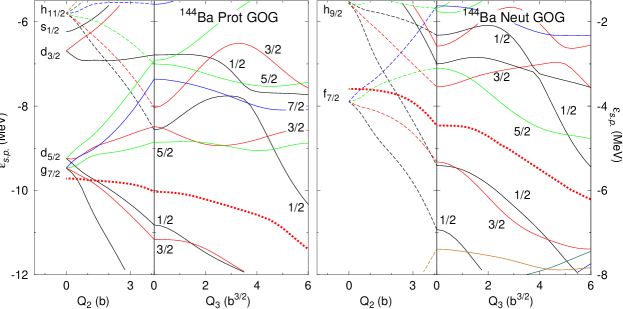
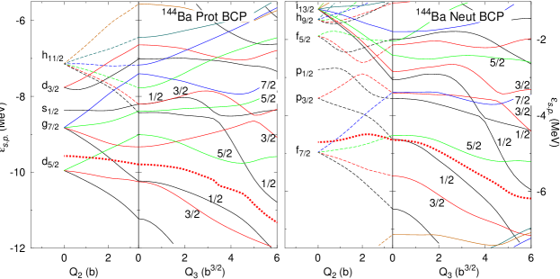
Figure 11: (Color online) Single particle energies (SPE) for the nucleus ¹⁴⁴Ba and computed with the BCP1 energy density functional (lower panels) and the Gogny D1S (upper panels) are plotted first as a function of the quadrupole moment $Q_{2}$ (in b) up to the value corresponding to the self consistent minimum at $Q_{3}=0$ ($Q_{2}=3.37$ b for the results obtained with the BCP1 functional and 4.12 b for the ones with the Gogny D1S force) and from there one as a function of the octupole moment $Q_{3}$(in b^3/2) (see the caption of Fig 3 for further details).

In Fig 10 the particle-particle correlation energies are plotted as a function of the octupole moment. As in the case of the radium isotopes, we observe that the general trend of $E_{pp}$ both for protons and neutrons and the two interaction/functional considered is to decrease for increasing octupole moments in the relevant interval between $Q_{3}=0$ b^3/2 and $Q_{3}\approx 3.5\textrm{b}^{3/2}$; a tendency that is also observed at higher values of the octupole moment in most of the barium isotopes studied. Based on the results of Fig. 10 as well as the ones of Fig 2 for the radium isotopes it is possible to say, in a very broad sense, that the onset of octupole deformation tends to quench pairing correlations and this quenching is bigger for larger values of the octupole moment. It is also noticed that in most of the cases the pairing correlation energies obtained in the BCP1 calculation are smaller than the ones obtained with the Gogny D1S force.

In Fig. 11 the SPE spectrum of ¹⁴⁴Ba obtained with the two kinds of interactions/functionals is shown. The meaning of the different panels is the same as in Fig. 3 for ²²⁴Ra. Here, the same comments made in the analysis and discussion of Fig. 3 for ²²⁴Ra and regarding the Nilsson quantum number contents of the single particle wave functions are also in order. Coming back to the plot, we observe in the proton spectra the presence near the Fermi level of an occupied positive parity $d_{5/2}$ spherical orbital and a nearby empty negative parity $h_{11/2}$ orbital. As discussed in the introduction, this is a characteristic property of the nuclear SPE for the octupole deformation to take place. In the SPE for neutrons we observe negative parity orbitals coming from the $f_{7/2}$ sub-shell below the Fermi level and positive parity orbitals coming from the $i_{13/2}$ above, which is again a characteristic signature of octupole deformation. We also observe that the Fermi level both for protons and neutrons is located in a region of low level density in the case of the Gogny force calculations, which is a required condition for octupole deformation to take place (Jahn-Teller effect). In the case of the calculations with BCP1 we observe that the Fermi level of neutrons is located in a region of moderate density of levels that could explain the lack of octupole deformed minima in the BCP1 calculations.

As in the ²²⁴Ra case, the position of the single particle levels cannot be used to assign the quantum numbers of neighboring odd-A nuclei in a fashion similar to the Nilsson diagram case.

Figure 12: Same as Fig. 7 but for the even-even barium isotopes with A in the range from 140 till 150.

In Fig. 12 the energies of the $1^{-}$ states and the transition probabilities obtained after solving the CSE are shown as a function of the mass number of the barium isotopes considered. In the left hand side panel the excitation energy of the $1^{-}$ state is plotted along with the available experimental data Phillips.96 ; Urban.97 ; Shneidman.05 ; Biswas.05 . We observe how the isotopic trend is reasonably well reproduced although the absolute values of the energies are typically a factor of two larger than the experimental values. The BCP1 excitation energies are closer to the ones from Gogny D1S than in the radium isotopes calculations. As discussed previously, the values of the energies strongly depend upon the values of the collective mass in the vicinity of the minimum as well as on the height and width of the barrier separating the two minima with opposite octupole deformation. Consequently, those excitation energies depend on the interaction/functional used as well as the level of detail of the theoretical description (inclusion of pairing correlations, restoration of symmetries) and therefore the discrepancy with the experiment is not very relevant. Concerning the $B(E1)$ values, we observe a dip in ¹⁴⁶Ba which is caused by the same effect as the dip in ²²⁴Ra, namely the peculiar behavior of the dipole moment $D_{0}(Q_{3})$ with the octupole moment and mass number. The BCP1 values for the $B(E1)$ transition probabilities are systematically smaller than the Gogny D1S ones by almost one order of magnitude. As in the case of the excitation energies of the $1^{-}$ states, it has to be stressed that the isotopic trend is consistent in the two sets of calculations and both nicely reproduced the scarce experimental data Butler.91 ; Phillips.96 . Finally, in the right hand side panel of Fig. 12 the $B(E3)$ transition probabilities are plotted. In this case and to our knowledge, no experimental data is available. The $B(E3)$ values show a not very smooth behavior that, on the other hand, is inversely correlated with the excitation energies of the $1^{-}$ states. Therefore the bigger $B(E3)$ values are obtained for the nuclei with the lower $1^{-}$ excitation energies.

III.3 Fission valley properties of ²⁴⁰Pu

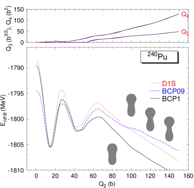
Figure 13: (Color online) In the lower panel the axially symmetric fission path (mean field energy versus axial quadrupole moment in barns) for the nucleus ²⁴⁰Pu and the three interactions/functionals considered (BCP1 full line, BCP2 dashed line, Gogny D1S dotted line). The shapes depicted correspond to the half-density contour line of the actual matter density distribution and are plotted such that their symmetry axis is located at the corresponding $Q_{20}$ value. In the upper panel the octupole and hexadecapole moments of the corresponding mean field states. Apparently, there are only two curves but this is because the results for the three functionals/interactions lie one on top of each other.

In this section the fission properties of ²⁴⁰Pu, regarding the octupole contents of the mean field configuration in its way out to scission, are analyzed for the two BCP functionals Baldo.08 and the Gogny D1S force. This isotope has been chosen as a paradigmatic example of fissioning nucleus that has been thoroughly studied with the Gogny force Berger.84 . As it is customary, the theoretical description of fission is based on the analysis of the potential energy curve (PEC) obtained by performing constrained mean field calculations with the quadrupole moment $Q_{2}=\langle Q_{20}\rangle$ as constraining quantity. Details on the procedures involved can be found in the literature Berger.84 ; Warda.02 ; Dubrai.08 . The PECs obtained in this case for the nucleus ²⁴⁰Pu are shown in the lower panel of Fig. 13. The range of quadrupole moments considered starts at sphericity ($Q_{2}=0$) and goes up to values corresponding to very elongated configurations closed to fission ($Q_{2}=150$ b). At $Q_{2}\approx 70$ b the matter distribution starts to resemble the form of two fission fragments connected by a neck as can be observed in the shapes given in the figure corresponding to the contour lines of the matter distribution at half density (see caption for further details). As the quadrupole moment increases, the distance between the fragments also increases and the width of the neck decreases. As a consequence, the energy roughly corresponds to the dominant Coulomb repulsion between the two incipient fragments. We observe how the results obtained with BCP and Gogny D1S are fairly similar with the position of the ground state minimum and the fission isomer lying at roughly the same $Q_{2}$ values. The potential energy curves obtained with the BCP1 and BCP2 functionals are very similar and are hardly distinguishable in Fig. 13. The fission isomer obtained with Gogny D1S lies at an excitation energy almost 2 MeV higher than the one obtained with the BCP functionals. It is also observed that the first and second fission barrier heights obtained with the Gogny D1S force are higher than the ones obtained from the BCP functionals. This is very likely a consequence of the surface coefficient in semi-infinite nuclear matter that is higher in Gogny D1S than in the BCP functionals (see the values quoted in robledo.08 ). At this point and taking into account the differences in the PECs it can be concluded that the predictions for the spontaneous fission half lives obtained with the BCP functionals and Gogny D1S force are going to be higher for Gogny D1S than for BCP. However, a definitive answer to this question can not be given until the effect of triaxiality has been incorporated into the calculations because it is well known that triaxiality can have a strong impact in the first barrier height. Also, it has to be kept in mind that the collective mass along the $Q_{2}$ collective degree of freedom, and entering the WKB formula used to estimate fission half lives, can be substantially different when computed with the BCP functionals or the Gogny D1S force. Therefore, the detailed discussion of the fission half lives obtained with the BCP functionals is deferred to a more detailed study of fission properties obtained with this class of functionals. In this paper, devoted to octupole deformation, it is enough to confirm that the shapes of the nucleus in its way down to fission are essentially the same irrespective of the functional/interaction used as can be seen in the upper panel of Fig. 13. In this plot, the octupole and hexadecapole moments are depicted as a function of $Q_{2}$ and, as can be observed, the curves for different interactions/functionals are indistinguishable of each other. This fact implies that the mass distribution close to scission (as depicted in Fig. 13 through the half density contours) is the same irrespective of the interaction/functional used in the calculation and therefore the predictions of the fission fragment mass distributions obtained at the mean field level with Gogny D1S force and BCP functionals should coincide.

IV Conclusions

We have explored the octupole degree of freedom in two sets of isotopes with the newly postulated BCP functionals. The agreement found with both experiment and the benchmark results obtained in the same framework with the Gogny D1S interaction, gives us confidence on the good properties of the BCP functionals concerning odd parity multipole moments. In addition, the matter distribution of the fissioning nucleus ²⁴⁰Pu, which strongly depend upon the response of the system to octupole perturbations, is found to be essentially the same in the three calculations performed implying thereby that the BCP functionals and the Gogny D1S force are equally well suited in that respect. Taking into account the microscopic origin of the BCP functionals it is comforting and encouraging to observe its good performance in properties like octupolarity that belong to the realm of finite nuclei.

- (1) A. Bohr and B.R. Mottelson, Nuclear Structure (Benjamin, New York, 1969 and 1975)
- (2) P. Ring and P. Shuck, The Nuclear Many Body Problem (Springer–Verlag Edt. Berlin, 1980)
- (3) M. Bender, P.-H. Heenen and P.-G. Reinhard, Rev. Mod. Phys. 75, 121 (2003)
- (4) P.A. Butler and W. Nazarewicz, Rev. Mod. Phys. 66, 349 (1996)
- (5) Hans J. Specht, Rev. Mod. Phys. 46, 773 (1974); S. Bjrnholm and J. E. Lynn, Rev. Mod. Phys. 52, 725 (1980)
- (6) M. Baldo, P. Schuck, X. Viñas, Phys. Lett. B 663, 390 (2008)
- (7) M. Baldo, C. Maieron, P. Schuck and X. Viñas, Nucl. Phys. A736, 241 (2004)
- (8) S.A. Fayans, JETP Lett. 68, 169 (1998)
- (9) S.A. Fayans and D. Zawischa, Int. J. Mod. Phys. B 15, 1684 (2001)
- (10) T. Duguet, M. Bender, K. Bennaceur, D. Lacroix, and T. Lesinski, Phys. Rev. C 79, 044320 (2009)
- (11) L. M. Robledo, M. Baldo, P. Schuck, and X. Viñas, Phys. Rev. C 77, 051301 (2008)
- (12) E. Garrido, P. Sarriguren, E. Moya de Guerra and P. Schuck, Phys. Rev. C 60, 064312 (1999)
- (13) J. Decharge and D. Gogny, Phys. Rev. C21, 1568 (1980)
- (14) J.F. Berger, M. Girod and D. Gogny. Nucl. Phys. A428, 23c (1984)
- (15) L. M. Robledo, J. L. Egido, J. F. Berger and, M. Girod, Phys. Lett. B187, 223 (1987)
- (16) J.L. Egido and L.M. Robledo, Nucl. Phys. A494, 85 (1989)
- (17) J.L. Egido and L.M. Robledo, Nucl. Phys. A518, 475 (1990)
- (18) P. Bonche, P. H. Heenen, H. Flocard and D. Vautherin, Phys. Lett. B175, 387 (1986)
- (19) D. Brink and W. Weiguny, Nucl. Phys. A120, 59 (1968)
- (20) B. Giraud and B. Grammaticos, Nucl. Phys. A233, 373 (1974)
- (21) P-G. Reinhard and K. Goeke, Rep. Prog. Phys. 50, 1 (1987)
- (22) M. Baranger and M. Veneroni, Ann. of Phys. 114, 123 (1978)
- (23) D.M. Brink, M.J. Giannoni and M. Veneroni, Nucl. Phys. A258, 237 (1976)
- (24) F. Villars, Nucl. Phys. A285, 269 (1977)
- (25) B. Nerlo–Pomorska, K. Pomorski, M. Brack and E. Werner, Nucl. Phys. A462, 252 (1987)
- (26) F. Villars, Nuclear Selfconsistent fields, Eds. G. Ripka and M. Porneuf (North Holland 1975)
- (27) P.G. Reinhard and K. Goeke, J. of Phys. G4, 245 (1978)
- (28) M. Girod and B. Grammaticos, Nucl. Phys. A330, 40 (1979)
- (29) A. Baran, K. Pomorski, A. Lukasiak and A. Sobiczewski, Nucl. Phys. A361, 83 (1981)
- (30) K. Boning, A. Sobiczewski, B. Nerlo-Pomorska and K. Pomorski, Phys. Lett. B161, 231 (1985).
- (31) J.L. Egido and L.M. Robledo, Nucl. Phys. A524, 65 (1991)
- (32) P. A. Butler and W. Nazarewicz, Nucl. Phys. A533, 249 (1991)
- (33) T. Kibédi and R. H. Spear, Atom. Data and Nucl. Data Tables, 80, 35 (2002)
- (34) R.H. Spear and W.N. Catford, Phys. Rev. C41, R1351 (1990)
- (35) V. Martin and L.M. Robledo, Phys. Rev C49, 188 (1994)
- (36) E. Garrote, J.L.Egido and L.M. Robledo, Phys. Lett. B410, 86 (1997)
- (37) E. Garrote, J.L. Egido and L.M. Robledo, Phys. Rev. Lett. 80, 4398 (1998)
- (38) W.R. Phillips, I. Ahmad, H. Emling, R. Holzmann, R.V.F. Janssens, T.-L. Khoo and M.W. Drigert, Phys. Rev. Lett 57, 3257 (1986)
- (39) T.M. Shneidman, R.V. Jolos, R. Krücken, A. Aprahamian, D. Cline, J.R. Cooper, M. Cromaz, R.M. Clark, C. Hutter, A.O. Macchiavelli, W. Scheid, M.A.Stoyer and C.Y. Wu, Eur. Phys. J. A25, 387 (2005)
- (40) W. Urban, M.A. Jones, J.L. Durell, M. Leddy, W.R. Phillips, A.G. Smith, B.J. Varley, I. Ahmad, L.R. Morss, M. Bentaleb, E. Lubkiewicz, and N. Schulz, Nucl. Phys. A613, 107 (1997)
- (41) D. C. Biswas, A. G. Smith, R. M. Wall, D. Patel, G. S. Simpson, D. M. Cullen, J. L. Durell, S. J. Freeman, J. C. Lisle, J. F. Smith, B. J. Varley, T. Yousef, G. Barreau, M. Petit, Ch. Theisen, E. Bouchez, M. Houry, R. Lucas, B. Cahan, A. Le Coguie, B. J. P. Gall, O. Dorvaux, and N. Schulz, Phys. Rev. C 71, 011301 (2005)
- (42) M. Warda, J.L. Egido, L.M. Robledo and K. Pomorski, Phys. Rev. C66, 014310 (2002); Intl. J. of Mod. Phys. E13, 169 (2004)
- (43) N. Dubray, H. Goutte, and J.-P. Delaroche, Phys. Rev. C77, 014310 (2008)