CPHT-RR016.0310,  DESY 10-041, LPT-Orsay-10-21
The transverse spin structure of the pion at short distances

1 Introduction

The structure of the pion at short distances unites two characteristic features of quantum chromodynamics. On the one hand, the pion plays a unique role among hadrons as the Goldstone boson of spontaneous chiral symmetry breaking. On the other hand, asymptotic freedom is central for understanding its structure at short distances, where quarks and gluons interact perturbatively as in any other hadron. Moreover, many studies of hadron structure are very much simplified when one deals with spin-zero hadrons, and the pion is probably the spin-zero hadron for which most quantitative information is available, both from experiment and from calculations in lattice QCD. A versatile tool to describe hadronic structure is given by generalized parton distributions or, equivalently, by the form factors of a tower of local quark-gluon operators containing an increasing number of covariant derivatives.

A perhaps surprising feature of the pion is that is has a non-trivial spin structure. An instructive quantity to describe this structure is the distribution $\rho(x,\boldsymbol{b})$ of quarks with longitudinal momentum fraction $x$ and transverse distance $\boldsymbol{b}$ from the center of the pion [1]. Due to parity invariance this distribution cannot depend on the longitudinal quark polarization. However, the distribution of quarks with transverse spin $\boldsymbol{s}$ has a polarization dependent part, which is proportional to $(\boldsymbol{s}\times\boldsymbol{b})^{z}$ and was found to be sizeable in a recent lattice study [2]. This polarization dependence can be quantified by the form factors of the quark tensor operator $\bar{q}\mskip 1.5mui\sigma^{\alpha\beta}\mskip 1.5muq$ and its analogs containing covariant derivatives. The present work is concerned with these tensor form factors at high momentum transfer, or in other words with the correlation between the transverse polarization and the transverse position of quarks very close to the center of the pion.

Form factors at high momentum transfer have played a key role in the early development of methods for calculating exclusive observables in QCD [3, 4]. They continue to provide an important area for applying factorization, with close links to the physics of exclusive $B$ meson decays. In the limit of infinite momentum transfer $Q^{2}$ form factors can be described within standard collinear factorization, but extensive studies of the electromagnetic pion form factor $F_{\pi}(Q^{2})$ indicate that at experimentally accessible values of $Q^{2}$ this description receives important corrections, see for instance [5, 6, 7, 8, 9]. In the present work we aim at providing a baseline for the large $Q^{2}$ behavior of the pion tensor form factors $B_{Tni}$, and we will use a very simplified extension of the collinear factorization framework that allows us to obtain expressions in compact analytical form. We do therefore not expect our results to be quantitatively reliable at moderately large $Q^{2}$, and we will in particular refrain from comparing to the lattice calculations in [2], which go up to $Q^{2}\approx 2.5\operatorname{GeV}^{2}$. On the other hand, our analytic expressions may be of use if one wants to devise parameterizations of $B_{Tni}(Q^{2})$ that have the correct behavior at large $Q^{2}$.

The large $Q^{2}$ behavior of pion tensor form factors is also interesting because it involves pion distribution amplitudes of twist three, which have a particular behavior at the end-points of the momentum fraction variable [10]. We find that for certain form factors $B_{Tni}$ the formulae obtained by using collinear factorization have end-point divergences and hence need to be modified. This is similar to other cases where twist-three pion distribution amplitudes appear, such as spectator interactions in exclusive $B$ decays [11, 13], pion electroproduction $ep\to e\pi^{+}n$ with transverse polarization of the exchanged virtual photon [14], and certain power corrections to $F_{\pi}(Q^{2})$ [15, 16].

This paper is organized as follows. In the next section we set up the calculational framework used in the present work. In Sect. 3 we extract the contributions from the hard-scattering graphs that dominate in the large $Q^{2}$ limit and derive simple analytic expressions for the form factors $B_{Tni}$. In Sect. 4 we present some numerical illustrations of our results, and in Sect. 5 we summarize our findings.

2 Setting up the calculation

The tensor form factors of the pion parameterize the matrix elements of the local operators

$$\operatorname{T}\underset{(\alpha,\beta_{1})}{\operatorname{A}}\;\underset{(\beta_{1},\ldots,\beta_{n})}{\operatorname{S}}\bar{q}\,i\sigma^{\alpha\beta_{1}}\,i{D^{\raisebox{2.41112pt}{$\scriptstyle\leftrightarrow$}}}{}^{\beta_{2}}\cdots\,i{D^{\raisebox{2.41112pt}{$\scriptstyle\leftrightarrow$}}}{}^{\beta_{n}}\mskip 1.5muq\,,$$ (1)

where ${D^{\raisebox{2.41112pt}{$\scriptstyle\leftrightarrow$}}}{}^{\beta}={\partial^{\raisebox{2.41112pt}{$\scriptstyle\leftrightarrow$}}}{}^{\beta}-igA^{\beta}$ with ${\partial^{\raisebox{2.41112pt}{$\scriptstyle\leftrightarrow$}}}{}^{\beta}={\textstyle\frac{1}{2}}({\partial^{\raisebox{2.41112pt}{$\scriptstyle\rightarrow$}}}{}^{\beta}-{\partial^{\raisebox{2.41112pt}{$\scriptstyle\leftarrow$}}}{}^{\beta})$ is the covariant derivative. Here $S$ and $A$ respectively denote symmetrization and antisymmetrization in the indicated indices, and $T$ denotes the subtraction of traces in all index pairs. These operations, which project on operators with twist two, can be implemented in a simple way by contraction with two constant auxiliary vectors $a$, $b$ satisfying $a^{2}=ab=0$ and $b^{2}\neq 0$ [17]. The tensor form factors are then given by

$$\langle\pi^{+}(p^{\prime})\,\big{|}\,\bar{u}\mskip 1.5mui\sigma^{\alpha\beta}a_{\alpha}b_{\beta}\,(i{D^{\raisebox{2.41112pt}{$\scriptstyle\leftrightarrow$}}}{}a)^{n-1}\mskip 1.5muu\,\big{|}\,\pi^{+}(p)\rangle=(aP)^{n-1}$$

$$\quad\times\frac{(ap)(bp^{\prime})-(bp)(ap^{\prime})}{m_{\pi}}\,\sum_{\genfrac{}{}{0.0pt}{}{i=0}{\text{even}}}^{n-1}(2\xi)^{i}\mskip 1.5muB_{Tni}^{u}(Q^{2})$$ (2)

with $Q^{2}=-(p-p)^{2}$ and

$$P =\frac{1}{2}(p+p^{\prime}), \xi =\frac{a(p-p^{\prime})}{a(p+p^{\prime})}.$$ (3)

The form factors in (2) refer to $u$-quarks; those for $d$-quarks follow from isospin symmetry and read

$$B^{d}_{Tni} =(-1)^{n}\mskip 1.5muB^{u}_{Tni}.$$ (4)

The form factors can be written as Mellin moments of generalized parton distributions of the pion as shown in [17], but we will not need this representation here.

In the collinear factorization formalism and at leading order in $\alpha_{s}$ the matrix element (2) receives contributions from the graphs in figure 1. Due to the covariant derivatives, the operator (1) contains terms with zero to $n-1$ gluon fields. Graphs (a) and (b) correspond to the term without gluon fields, i.e. to

$$\bar{u}\mskip 1.5mui\sigma^{\alpha\beta}a_{\alpha}b_{\beta}\,(i{\partial^{\raisebox{2.41112pt}{$\scriptstyle\leftrightarrow$}}}{}a)^{n-1}\mskip 1.5muu$$ (5)

in (2). The same graphs describe the electromagnetic pion form factor if one inserts the electromagnetic current instead of the current in (5). Graph (c) corresponds to the terms in (1) that have exactly one gluon field, i.e. to

$$\sum_{j=1}^{n-1}\bar{u}\mskip 1.5mui\sigma^{\alpha\beta}a_{\alpha}b_{\beta}\,(i{\partial^{\raisebox{2.41112pt}{$\scriptstyle\leftrightarrow$}}}{}a)^{n-1-j}(gAa)\,(i{\partial^{\raisebox{2.41112pt}{$\scriptstyle\leftrightarrow$}}}{}a)^{j-1}\mskip 1.5muu$$ (6)

in (2). Terms with more than one gluon field do not contribute at this level.

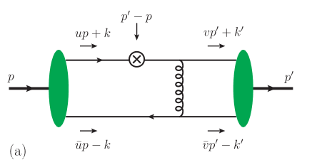
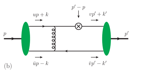
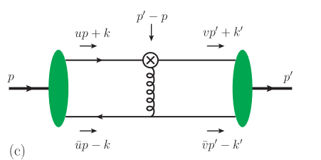
Figure 1: Graphs for the matrix element (2) in the limit of large $Q^{2}$. The crossed circle represents the insertion of the relevant current operator, given by (5) for graphs (a) and (b) and by (6) for graph (c). The blobs stand for the sum of twist-two and twist-three distribution amplitudes as specified in (2).

When calculating the hard-scattering part of the graphs we neglect the pion mass, so that the pion momenta $p$ and $p^{\prime}$ are purely lightlike. We use them to define the two light-cone directions required for specifying the distribution amplitudes of the pions, working in a reference frame where the incoming pion moves in the positive and the outgoing pion in the negative $z$ direction. As indicated in the figure, we write the $u$-quark momentum as $up+k$ in the incoming $\pi^{+}$ and as $vp^{\prime}+k^{\prime}$ for the outgoing $\pi^{+}$, with the light-cone momentum fractions $u$ and $v$ ranging from $0$ to $1$. The vectors $k$ and $k^{\prime}$ are transverse to both $p$ and $p^{\prime}$. We neglect the small momentum components of the quarks and antiquarks, i.e. the component along $p^{\prime}$ in the incoming pion and the component along $p$ in the outgoing one. Note that $(up+k)^{2}=k^{2}$ and $(vp^{\prime}+k^{\prime})^{2}=k^{\prime 2}$ are in general not zero—we will comment on this shortly.

Since the tensor operators (1) have odd chirality, we need one chiral-even and one chiral-odd pion distribution amplitude in the graphs to obtain a nonvanishing hard-scattering amplitude. Since there is no chiral-odd pion distribution amplitude with twist two, we must go to twist-three level. The relevant distribution amplitudes have been introduced in [10]. After a Fourier transform from the position representation used in [10] to momentum space, the projection operators for the incoming and the outgoing pion respectively read [11]

$$\Phi\Bigl{(}u,\frac{\partial}{\partial k}\Bigr{)}=-\frac{if_{\pi}}{4}\biggl{\{}\phi(u)\mskip 1.5mu\not{p}\gamma_{5}+\mu_{\pi}\mskip 1.5mu\phi_{p}(u)\mskip 1.5mu\gamma_{5}$$

$$\ +\mu_{\pi}\mskip 1.5mu\frac{i\sigma^{\alpha\beta}\gamma_{5}}{6}\biggl{[}\frac{d\phi_{\sigma}(u)}{du}\,\frac{p_{\alpha}\mskip 1.5mup^{\prime}\!\mskip-1.5mu{}_{\beta}}{pp^{\prime}}-\phi_{\sigma}(u)\,p_{\alpha}\mskip 1.5mu\frac{\partial}{\partial k^{\beta}}\biggr{]}\biggr{\}}\,,$$

$$\Phi^{\prime}\Bigl{(}v,\frac{\partial}{\partial k^{\prime}}\Bigr{)}=\frac{if_{\pi}}{4}\biggl{\{}\phi(v)\mskip 1.5mu\not{p}^{\prime}\gamma_{5}-\mu_{\pi}\mskip 1.5mu\phi_{p}(v)\mskip 1.5mu\gamma_{5}$$

$$\ +\mu_{\pi}\mskip 1.5mu\frac{i\sigma^{\alpha\beta}\gamma_{5}}{6}\biggl{[}\frac{d\phi_{\sigma}(v)}{dv}\,\frac{p^{\prime}\!\mskip-1.5mu{}_{\alpha}\mskip 1.5mup_{\beta}}{pp^{\prime}}-\phi_{\sigma}(v)\,p^{\prime}\!\mskip-1.5mu{}_{\alpha}\mskip 1.5mu\frac{\partial}{\partial k^{\prime\beta}}\biggr{]}\biggr{\}}$$ (7)

with $f_{\pi}=130.4\operatorname{MeV}$ [12] and

$$\mu_{\pi}=\frac{m_{\pi}^{2}}{m_{u}+m_{d}}.$$ (8)

In (8) the pion mass can of course not be neglected since one is dealing with a non-perturbative quantity. For the twist-three distribution amplitudes we take the asymptotic forms under evolution,

$$\phi_{p}(u) =1, \phi_{\sigma}(u) =6u\bar{u},$$ (9)

where here and in the following we use the notation

$$\bar{u}=1-u.$$ (10)

The normalization constant $f_{3\pi}$ associated with the twist-three quark-gluon-quark distribution amplitudes of the pion asymptotically evolves to zero [10]. In the limit where $\phi_{p}$ and $\phi_{\sigma}$ take the form (9), the graphs in figure 1 therefore give the full answer for the matrix element (2). Conversely, the consideration of distribution amplitudes deviating from (9) would require the inclusion of graphs with an additional gluon in one of the pion distribution amplitudes and thus considerably complicate the analysis. Since in this work we aim at understanding the basic behavior of the form factors at large $Q^{2}$, we consider the restriction to the asymptotic forms (9) to be sufficient. On the other hand, we can easily keep the general form

$$\phi(u)=6u\bar{u}\mskip 1.5mug(u)$$ (11)

of the twist-two distribution amplitude, where

$$g(u)=1+\sum_{n=2}^{\infty}a_{n}\mskip 1.5muC_{n}^{3/2}(u-\bar{u})$$ (12)

is the usual expansion in Gegenbauer polynomials, with coefficients $a_{n}$ that evolve with a simple multiplicative factor at leading order [3, 4]. With (9) to (12) the factorization scale dependence of the projectors (2) is then given by

$$\mu_{\pi}(\mu) =\mu_{\pi}(\mu_{0})\,\biggl{(}\frac{\alpha_{s}(\mu_{0})}{\alpha_{s}(\mu)}\biggr{)}^{4/\beta_{0}},$$

$$a_{n}(\mu) =a_{n}(\mu_{0})\,\biggl{(}\frac{\alpha_{s}(\mu_{0})}{\alpha_{s}(\mu)}\biggr{)}^{-\gamma_{n}/\beta_{0}}$$ (13)

at leading logarithmic accuracy, where $\alpha_{s}(\mu)$ is the one-loop running coupling, $\beta_{0}=11-2n_{F}/3$, and the first few anomalous dimensions read $\gamma_{2}=50/9$, $\gamma_{4}=364/45$, etc. The scale dependence of $\mu_{\pi}$ simply reflects the running of the quark masses in (8).

An alternative form of the projector (2) was derived in section 3.2 of [13], which had earlier been used in [15, 16]. This derivation requires one to keep the small components of the quark and antiquark momenta in the intermediate stages of the calculation and to adjust them such that both the quark and the antiquark attached to the pion wave function are exactly on shell. Having the external quarks and antiquarks of the hard-scattering subprocess exactly on shell is certainly an attractive feature of the calculation, especially from the point of view of gauge invariance. It comes, however, at the price of violating momentum conservation. Consider for definiteness the quark and antiquark momenta in the incoming pion:

$$k_{q} =up+k+w_{q}\mskip 1.5mup^{\prime}, k_{\bar{q}} =\bar{u}p-k+w_{\bar{q}}\mskip 1.5mup^{\prime}.$$ (14)

For generic values of $u$ and $k$ one cannot have both $k_{q}^{2}=k_{\bar{q}}^{2}=0$ and $w_{q}+w_{\bar{q}}=0$ (for this it does not matter whether one neglects the pion mass or not). In our calculation, we choose to be consistent with momentum conservation neglect the small components $w_{q}\mskip 1.5mup^{\prime}$ and $w_{\bar{q}}\mskip 1.5mup^{\prime}$. We will explicitly check that gauge invariance holds for the class of covariant gauges and within the accuracy of our calculation.

As explained in [11], the derivatives with respect to $k$ and $k^{\prime}$ in the projector (2) act on the hard-scattering kernel before one takes the collinear limit by setting $k=k^{\prime}=0$. However, we will see that for some of the form factors $B_{Tni}^{u}$ the collinear limit cannot be taken since the integrals over $u$ and $v$ diverge at their end-points for $k=k^{\prime}=0$. To keep the intermediate steps of our calculation well-defined, we introduce transverse-momentum dependent factors $\Sigma(u,k^{2})$ and $\Sigma(v,k^{\prime 2})$ for the incoming and outgoing pion. These factors are real-valued and normalized as

$$\int d^{2}k\;\Sigma(u,k^{2})=1.$$ (15)

In a more sophisticated approach, which has for instance been used in [14], one would multiply the different terms in $\Phi$ and $\Phi^{\prime}$ with different factors and interpret the result as pion light-cone wave functions that depend on both a longitudinal momentum fraction $u$ or $v$ and on the transverse parton momentum. Furthermore, in the spirit of the modified hard-scattering approach, one should include Sudakov factors for each pion, which resum a class of large logarithms from higher-order corrections and depends on the momentum fractions, the transverse parton momenta and the hard scale $Q$ in a non-trivial way [6]. Formally, the Sudakov factors alone would already remove the end-point divergences of the $u$ and $v$ integrals, but for a wide range of hard scales $Q^{2}$ the resulting integrals will receive large contributions from phase space regions where parton virtualities are low and the perturbative expression of the Sudakov factors is not justified (see [18] for a detailed analysis of the situation in semileptonic $B\to\pi$ decays). Moreover, even a calculation with Sudakov factors but without a nonperturbative transverse-momentum dependence of the pion wave function would not readily yield simple analytic expressions. Since the latter is what we are aiming for in the present work, we will use a global factor $\Sigma(u,k^{2})\,\Sigma(v,k^{\prime 2})$ as a minimal version to regulate the intermediate steps of our calculation and simplify the resulting integrals in the end, see eq. (38) below.

With these preliminaries we can write the large-$Q^{2}$ limit of the matrix element we are interested in as

$$\langle\pi^{+}(p^{\prime})\,\big{|}\,\bar{u}\mskip 1.5mui\sigma^{\alpha\beta}a_{\alpha}b_{\beta}\,(i{D^{\raisebox{2.41112pt}{$\scriptstyle\leftrightarrow$}}}{}a)^{n-1}\mskip 1.5muu\,\big{|}\,\pi^{+}(p)\rangle$$

$$\quad=4\pi\alpha_{s}\frac{C_{F}}{N_{c}}\,6f_{\pi}^{2}\,\mu_{\pi}\int du\,dv\;d^{2}k\,d^{2}k^{\prime}\;\Sigma(u,k^{2})\,$$

$$\hskip 90.00014pt\times\Sigma(v,k^{\prime 2})\,f(u,v;k,k^{\prime})$$ (16)

with

$$f(u,v;k,k^{\prime})=\frac{1}{6f_{\pi}^{2}\,\mu_{\pi}}\,$$

$$\quad\times\operatorname{Tr}\Phi\Bigl{(}u,\frac{\partial}{\partial k}\Bigr{)}\,\gamma^{\lambda}\mskip 1.5mu\Phi^{\prime}\Bigl{(}v,\frac{\partial}{\partial k^{\prime}}\Bigr{)}\,\frac{D_{\lambda\mu}}{\bar{u}\bar{v}Q^{2}-(k-k^{\prime})^{2}}$$

$$\qquad\times\biggl{[}\gamma^{\mu}\,\frac{\not{p}^{\prime}-\bar{u}\not{p}+\not{k}}{\bar{u}Q^{2}-k^{2}}\,i\sigma^{\alpha\beta}\mskip 1.5mu(a\mskip 1.5mul_{u})^{n-1}$$

$$\qquad\quad+(a\mskip 1.5mul_{v})^{n-1}\mskip 1.5mui\sigma^{\alpha\beta}\,\frac{\not{p}-\bar{v}\not{p^{\prime}}+\not{k}^{\prime}}{\bar{v}Q^{2}-k^{\prime 2}}\,\gamma^{\mu}\phantom{\biggl{[}\biggr{]}}$$

$$\qquad\quad+i\sigma^{\alpha\beta}a^{\mu}\sum_{j=1}^{n-1}(a\mskip 1.5mul_{u})^{j-1}\mskip 1.5mu(a\mskip 1.5mul_{v})^{n-1-j}\biggr{]}\,a_{\alpha}b_{\beta}\,,$$ (17)

where the last three lines of (2) respectively correspond to graphs (a), (b) and (c) in figure 1. The factors

$$a\mskip 1.5mul_{u} ={\textstyle\frac{1}{2}}\mskip 1.5mu(u-\bar{u})\mskip 1.5muap+{\textstyle\frac{1}{2}}\mskip 1.5muap^{\prime}+ak =aP\mskip 1.5mu(u-\xi\bar{u})+ak,$$

$$a\mskip 1.5mul_{v} ={\textstyle\frac{1}{2}}\mskip 1.5mu(v-\bar{v})\mskip 1.5muap^{\prime}+{\textstyle\frac{1}{2}}\mskip 1.5muap+ak^{\prime} =aP\mskip 1.5mu(v+\xi\bar{v})+ak^{\prime}$$

come from the derivatives $i{\partial^{\raisebox{2.41112pt}{$\scriptstyle\leftrightarrow$}}}{}a={\textstyle\frac{1}{2}}\mskip 1.5mu(i{\partial^{\raisebox{2.41112pt}{$\scriptstyle\rightarrow$}}}{}-i{\partial^{\raisebox{2.41112pt}{$\scriptstyle\leftarrow$}}}{})a$ in the operators (5) and (6). The denominator of the gluon propagator in all three graphs is $\bar{u}\bar{v}Q^{2}-(k-k^{\prime})^{2}$, and the quark propagators in graphs (a) and (b) have denominators $\bar{u}Q^{2}-k^{2}$ and $\bar{v}Q^{2}-k^{\prime 2}$. Note that we are using a Minkowskian scalar product for the vectors $k$ and $k^{\prime}$, so that $k^{2}$, $k^{\prime 2}$ and $(k-k^{\prime})^{2}$ are negative. In Feynman gauge, the numerator of the gluon propagator is $D_{\lambda\mu}=g_{\lambda\mu}$ and the fermion trace evaluates to

$$f(u,v;k,k^{\prime})=\biggl{[}f_{1}+f_{2}+\frac{\partial}{\partial k^{\alpha}}\mskip 1.5mu\bigl{(}f_{3}^{\alpha}+f_{4}^{\alpha}-f_{5}^{\alpha}\bigr{)}\biggr{]}$$

$$\qquad\times(a\mskip 1.5mul_{u})^{n-1}\,\frac{\bar{u}}{\bar{u}Q^{2}-k^{2}}\,\frac{1}{\bar{u}\bar{v}Q^{2}-(k-k^{\prime})^{2}}$$

$$\quad+\biggl{[}f_{6}-\frac{\partial}{\partial k^{\alpha}}\mskip 1.5muf_{7}^{\alpha}\biggr{]}\;\sum_{j=1}^{n-1}(a\mskip 1.5mul_{u})^{j-1}\mskip 1.5mu(a\mskip 1.5mul_{v})^{n-1-j}\;$$

$$\qquad\times\frac{1}{Q^{2}}\,\frac{1}{\bar{u}\bar{v}Q^{2}-(k-k^{\prime})^{2}}$$

$$\quad-\biggl{\{}u\leftrightarrow v,p\leftrightarrow p^{\prime},k\leftrightarrow k^{\prime},\frac{\partial}{\partial k}\to\frac{\partial}{\partial k^{\prime}}\mskip 1.5mu,\xi\to-\xi\biggr{\}}$$

with

$$f_{1} =\Bigl{[}(ap)(bp^{\prime})-(bp)(ap^{\prime})\Bigr{]}\Bigl{(}ug(u)-\bar{u}\,v\bar{v}\mskip 1.5mug(v)\Bigr{)}\,,$$

$$f_{2} =\Bigl{[}(ap)(bk)-(bp)(ak)\Bigr{]}ug(u)$$

$$\quad-\Bigl{[}(ap^{\prime})(bk)-(bp^{\prime})(ak)\Bigr{]}v\bar{v}\mskip 1.5mug(v)\,,$$

$$f_{3}^{\alpha} =\Bigl{[}(ap)(bp^{\prime})-(bp)(ap^{\prime})\Bigr{]}\mskip 1.5muk^{\alpha}\,{u\,v\bar{v}}\,g(v)/{2}\,,$$

$$f_{4}^{\alpha} =\Bigl{[}\mskip 1.5mua^{\alpha}\mskip 1.5mu(bk)-b^{\alpha}\mskip 1.5mu(ak)\Bigr{]}\mskip 1.5mu(pp^{\prime})\,{u\,v\bar{v}}\,g(v)/{2}\,,$$

$$f_{5}^{\alpha} =\Bigl{[}\mskip 1.5mua^{\alpha}\mskip 1.5mu(bp)-b^{\alpha}\mskip 1.5mu(ap)\Bigr{]}\mskip 1.5mu(pp^{\prime})\,u\bar{u}\,v\bar{v}\mskip 1.5mug(v)\,,$$

$$f_{6} =\Bigl{[}(ap)(bp^{\prime})-(bp)(ap^{\prime})\Bigr{]}\mskip 1.5mu(ap)\,(v-\bar{v})\,u\bar{u}\mskip 1.5mug(u)\,,$$

$$f_{7}^{\alpha} =\Bigl{[}\mskip 1.5mua^{\alpha}\mskip 1.5mu(bp)-b^{\alpha}\mskip 1.5mu(ap)\Bigr{]}\mskip 1.5mu(pp^{\prime})(ap^{\prime})\,u\bar{u}\,v\bar{v}\mskip 1.5mug(v)\,,$$ (20)

where we have split the result into different terms to facilitate the subsequent discussion.

In (2) it is understood that the derivatives $\partial/\partial k^{\alpha}$ act also on the vectors $k$ that are implicit in the functions $f_{i}^{\alpha}$ and in the factors $(a\mskip 1.5mul_{u})$. Likewise, the exchange of variables indicated in the last line of (2) applies also to the functions $f_{i}$, $f_{i}^{\alpha}$ and the factors $(a\mskip 1.5mul_{u})$ and $(a\mskip 1.5mul_{v})$.

One can recognize from the factors $g(u)$ and $g(v)$ in (2) that the hard-scattering graphs with the insertion of the chiral-odd operators (5) and (6) pick out a twist-two distribution amplitude in one of the two pions and a twist-three distribution amplitude in the other, as anticipated earlier.

3 Extracting the leading terms

The factorization formalism is based on an expansion in the small parameter $\Lambda/Q$, where $\Lambda$ stands for nonperturbative momentum scales. In this section we will extract the leading terms in this expansion.

In the following we will assume that the Gegenbauer series for $g(u)$ in (12) converges in the interval $u\in[0,1]$, so that $\phi(u)$ in (11) vanishes linearly at the end-points. The possibility that this may not hold for low or moderate factorization scales $\mu$ has been discussed in a number of papers, see for instance [19, 20, 21, 22, 23]. However, the anomalous dimensions $\gamma_{n}$ in (2) are positive and increase for $n>0$, and evolution to high scales will eventually ensure the convergence of (12) irrespective of the starting conditions. Since we are interested in the large-$Q^{2}$ behavior, the assumption that $g(u)$ is finite at the end-points $u=0$ and $u=1$ is therefore justified.

Due to the denominators of quark and gluon propagators, the integrals over $u$ and $v$ in (2) can be divergent when $k$ and $k^{\prime}$ are zero. From (2) and (2) we see that these divergences are at most logarithmic in both $u$ and $v$. For the moment we will keep the transverse momenta $k$ and $k^{\prime}$ fixed, and regard them as of order $\Lambda\ll Q$ for the purpose of power counting. We first identify terms in (2) that after integration over $u$ and $v$ vanish like a power of $\Lambda/Q$ (possibly times a power of $\ln Q/\Lambda$). We neglect these terms since other contributions will turn out to be finite or to grow like a power of $\ln Q/\Lambda$ in the large-$Q^{2}$ limit.

To simplify expressions, we use that

$$\int d^{2}k\,d^{2}k^{\prime}\;k^{\alpha}\,s(k^{2},k^{\prime 2},kk^{\prime})=0$$ (21)

and

$$\int d^{2}k\,d^{2}k^{\prime}\;k^{\alpha}k^{\beta}\,s(k^{2},k^{\prime 2},kk^{\prime})$$

$$\quad=\frac{1}{2}\,g_{T}^{\alpha\beta}\int d^{2}k\,d^{2}k^{\prime}\;k^{2}\,s(k^{2},k^{\prime 2},kk^{\prime})$$ (22)

because of rotational invariance in the transverse plane, where $s$ is a scalar function and

$$g_{T}^{\alpha\beta}=g^{\alpha\beta}-\frac{p^{\alpha}\mskip 1.5mup^{\prime}{}^{\beta}+p^{\prime}{}^{\alpha}\mskip 1.5mup^{\beta}}{pp^{\prime}}.$$ (23)

Relations analogous to (21) and (3) hold with one or both of $k^{\alpha}$, $k^{\beta}$ replaced by $k^{\prime\alpha}$, $k^{\prime\beta}$.

We now discuss the different terms of (2) in turn. The reader not interested in the intermediate steps of the argument may skip forward to eq. (3). Let us start with the contribution involving $f_{4}^{\alpha}$. If the derivative $\partial/\partial k$ acts on the factors $(bk)$ and $(ak)$ in $f_{4}^{\alpha}$, the result is proportional to $\smash{a_{\alpha}\mskip 1.5mug_{T}^{\alpha\beta}b_{\beta}-b_{\alpha}\mskip 1.5mug_{T}^{\alpha\beta}a_{\beta}}$ and hence vanishes. If the derivatives act on a factor $(ak)$ in $(a\mskip 1.5mul_{u})$, one is left with at least two powers of $k$ or $k^{\prime}$ in the numerator (a single power giving zero after angular integration), which are multiplied by a term proportional to

$$\frac{\bar{u}}{\bar{u}Q^{2}-k^{2}}\,\frac{\bar{v}}{\bar{u}\bar{v}Q^{2}-(k-k^{\prime})^{2}}.$$ (24)

After integration over $u$ and $v$, this term behaves like $\ln Q/\Lambda$ times an even power of $\Lambda/Q$ and can hence be neglected as well. The terms where the derivative $\partial/\partial k$ acts on the propagator denominators are proportional to

$$\frac{(ak)(bk)}{\bar{u}Q^{2}-k^{2}}+\frac{(ak)(bk)-(ak^{\prime})(bk)}{\bar{u}\bar{v}Q^{2}-(k-k^{\prime})^{2}}-\bigl{\{}a\leftrightarrow b\bigr{\}}\\[1.99997pt] ={}-\frac{(ak^{\prime})(bk)-(bk^{\prime})(ak)}{\bar{u}\bar{v}Q^{2}-(k-k^{\prime})^{2}},$$ (25)

which vanishes after angular integration. The contribution from $f_{4}^{\alpha}$ can hence be neglected altogether.

We proceed with the contributions from $f_{5}^{\alpha}$ and $f_{7}^{\alpha}$. When $\partial/\partial k$ acts on a factor $(ak)$ in $(a\mskip 1.5mul_{u})$, we obtain

$$(pp^{\prime})\mskip 1.5mu\Bigl{[}(a_{\alpha}\,g_{T}^{\alpha\beta}a_{\beta})(bp)-(a_{\alpha}\,g_{T}^{\alpha\beta}b_{\beta})(ap)\Bigr{]}\\[1.00006pt] =(ap)\mskip 1.5mu\Bigl{[}(ap)(bp^{\prime})-(bp)(ap^{\prime})\Bigr{]}$$ (26)

multiplied by an expression that, due to the factors $\bar{u}$ and $\bar{v}$ in the numerator, gives a finite integral over $u$ and $v$ even if $k=k^{\prime}=0$. If, however, the derivative acts on the propagator denominators, we obtain a term proportional to

$$\frac{\bar{u}}{\bar{u}Q^{2}-k^{2}}\,\frac{\bar{u}\bar{v}}{\bar{u}\bar{v}Q^{2}-(k-k^{\prime})^{2}}\,\biggl{[}\frac{(ak)}{\bar{u}Q^{2}-k^{2}}\\[1.99997pt] +\frac{(ak)-(ak^{\prime})}{\bar{u}\bar{v}Q^{2}-(k-k^{\prime})^{2}}\biggr{]}(bp)-\bigl{\{}a\leftrightarrow b\bigr{\}}.$$ (27)

At least one more power of $(ka)$ from $(a\mskip 1.5mul_{u})$ is required to get a nonvanishing term after angular integration. The integrals over $u$ and $v$ are only logarithmically divergent, so that this contribution is suppressed by an even power of $\Lambda/Q$ and can again be neglected.

Let us now discuss the term with $f_{3}^{\alpha}$. The contribution from the derivative $\partial/\partial k$ acting on $k^{\alpha}$ needs to be retained, whereas contributions with the derivative acting on a factor $(ak)$ in $(a\mskip 1.5mul_{u})$ can be neglected: they have at least two powers of $k$ in the numerator, which are multiplied by an expression that gives only a logarithm $\ln Q/\Lambda$ after integration over $u$ and $v$. When the derivative acts on the propagator denominators, we get a term proportional to

$$\frac{\bar{u}}{\bar{u}Q^{2}-k^{2}}\,\frac{\bar{v}}{\bar{u}\bar{v}Q^{2}-(k-k^{\prime})^{2}}\,\biggl{[}\frac{k^{2}}{\bar{u}Q^{2}-k^{2}}\\[1.99997pt] +\frac{k\mskip 1.5mu(k-k^{\prime})}{\bar{u}\bar{v}Q^{2}-(k-k^{\prime})^{2}}\biggr{]}.$$ (28)

The integral over $v$ of this term gives a logarithm $\ln Q/\Lambda$, whereas the one over $u$ diverges linearly for $k=k^{\prime}=0$. For finite $k$ and $k^{\prime}$ the $u$-integral thus provides a factor $1/\Lambda^{2}$ that cancels the factor $\Lambda^{2}$ from the transverse momenta in the numerator. Note, however, that the expression in (28) is multiplied by $n-1$ powers of $(a\mskip 1.5mul_{u})=aP\mskip 1.5mu(u-\xi\bar{u})+ak$. Only the contributions from $(aP)u$ need to be retained, since a factor $\bar{u}$ turns the linearly divergent $u$-integral of (28) into a logarithmically divergent one, whereas factors of $(ak)$ directly provide further powers of $(\Lambda/Q)^{2}$.

After performing the derivatives $\partial/\partial k$ and $\partial/\partial k^{\prime}$ in (2), we can omit all terms $(ak)$ in $(a\mskip 1.5mul_{u})$ and $(ak^{\prime})$ in $(a\mskip 1.5mul_{v})$, since they give rise to power suppressed terms. Furthermore, the contribution from $f_{2}$ is power suppressed and can be neglected.

Putting everything together we have

$$\int du\,dv\,\;d^{2}k\,d^{2}k^{\prime}\;\Sigma(u,k^{2})\,\Sigma(v,k^{\prime 2})\,f(u,v;k,k^{\prime})$$

$$\ =\Bigl{[}(ap)(bp^{\prime})-(bp)(ap^{\prime})\Bigr{]}\mskip 1.5mu(aP)^{n-1}\phantom{\int}$$

$$\quad\times\int du\,dv\;d^{2}k\,d^{2}k^{\prime}\;\Sigma(u,k^{2})\,\Sigma(v,k^{\prime 2})\;$$

$$\quad\times\frac{1}{Q^{2}}\,\frac{1}{\bar{u}\bar{v}Q^{2}-(k-k^{\prime})^{2}}\,\biggl{(}\frac{\bar{u}Q^{2}}{\bar{u}Q^{2}-k^{2}}$$

$$\qquad\times\biggl{\{}\Bigl{[}ug(u)+(u-\bar{u})\,v\bar{v}\mskip 1.5mug(v)\Bigr{]}\mskip 1.5mu(u-\xi\bar{u})^{n-1}$$

$$\qquad\quad+u^{n}\mskip 1.5muv\bar{v}\mskip 1.5mug(v)\,\biggl{[}\frac{k^{2}}{\bar{u}Q^{2}-k^{2}}+\frac{k\mskip 1.5mu(k-k^{\prime})}{\bar{u}\bar{v}Q^{2}-(k-k^{\prime})^{2}}\biggr{]}$$

$$\qquad\quad-(1+\xi)\,u\bar{u}\,v\bar{v}\mskip 1.5mug(v)\mskip 1.5mu(n-1)(u-\xi\bar{u})^{n-2}\mskip 1.5mu\biggr{\}}\;$$

$$\qquad+(1+\xi)(v-\bar{v})\,u\bar{u}\mskip 1.5mug(u)\phantom{\frac{1}{1}}$$

$$\qquad\quad\times\sum_{j=1}^{n-1}(u-\xi\bar{u})^{j-1}\mskip 1.5mu(v+\xi\bar{v})^{n-1-j}$$

$$\qquad-(1-\xi^{2})\,u\bar{u}\,v\bar{v}\mskip 1.5mug(v)\phantom{\frac{1}{1}}$$

$$\qquad\quad\times\sum_{j=1}^{n-1}(j-1)(u-\xi\bar{u})^{j-2}\mskip 1.5mu(v+\xi\bar{v})^{n-1-j}\mskip 1.5mu\biggr{)}$$

$$\quad+\Bigl{\{}u\leftrightarrow v,k\leftrightarrow k^{\prime},\xi\to-\xi\Bigr{\}}+\mathcal{O}\biggl{(}\frac{\Lambda^{2}}{Q^{2}}\,\ln^{2}\frac{Q^{2}}{\Lambda^{2}}\biggr{)}.$$

Before proceeding let us mention that we checked the gauge independence of our result for a general covariant gauge. Using the same methods as those leading to (3), we find that the gauge dependent part of $D_{\lambda\mu}$ gives only contributions suppressed by an even power of $\Lambda/Q$.

Let us now rewrite (3) in a form that allows us to identify those terms that give logarithms in $Q/\Lambda$. For the term proportional to $v\bar{v}\mskip 1.5mug(v)$ in the fifth line of (3) we can write

$$(u-\bar{u})\,(u-\xi\bar{u})^{n-1}\phantom{\Bigl{[}\Bigr{]}}$$

$$\quad=1-2\bar{u}(u-\xi\bar{u})^{n-1}-\Bigl{[}1-(u-\xi\bar{u})^{n-1}\Bigr{]}$$

$$\quad=1-2\bar{u}(u-\xi\bar{u})^{n-1}-(1+\xi)\,\bar{u}\sum_{j=1}^{n-1}(u-\xi\bar{u})^{j-1},$$ (30)

where in the last step we have used the geometric series. Similarly, the terms proportional to $ug(u)$ in (3) can be rewritten as

$$(u-\xi\bar{u})^{n-1}\,\frac{\bar{u}Q^{2}}{\bar{u}Q^{2}-k^{2}}\phantom{\sum_{j}^{1}}$$

$$\quad+(1+\xi)\,(v-\bar{v})\,\bar{u}\sum_{j=1}^{n-1}(u-\xi\bar{u})^{j-1}\mskip 1.5mu(v+\xi\bar{v})^{n-1-j}$$

$$=(u-\xi\bar{u})^{n-1}\,\frac{\bar{u}Q^{2}}{\bar{u}Q^{2}-k^{2}}+(1+\xi)\,\bar{u}\sum_{j=1}^{n-1}(u-\xi\bar{u})^{j-1}$$

$$\quad{}-(1+\xi)\,\bar{u}\sum_{j=1}^{n-1}(u-\xi\bar{u})^{j-1}\Bigl{[}1-(v+\xi\bar{v})^{n-1-j}\Bigr{]}$$

$$\quad{}-2(1+\xi)\,\bar{v}\bar{u}\sum_{j=1}^{n-1}(u-\xi\bar{u})^{j-1}\mskip 1.5mu(v+\xi\bar{v})^{n-1-j}$$

$$=1+(u-\xi\bar{u})^{n-1}\,\frac{k^{2}}{\bar{u}Q^{2}-k^{2}}\phantom{\sum_{j}^{1}}$$

$$\quad{}-(1-\xi^{2})\,\bar{u}\bar{v}\sum_{j=1}^{n-1}(u-\xi\bar{u})^{j-1}\sum_{l=1}^{n-1-j}(v+\xi\bar{v})^{l-1}$$

$$\quad{}-2(1+\xi)\,\bar{u}\bar{v}\sum_{j=1}^{n-1}(u-\xi\bar{u})^{j-1}\mskip 1.5mu(v+\xi\bar{v})^{n-1-j}.$$ (31)

In the term proportional to $k^{2}$ we only need to keep the factor $u^{n-1}$, since with one or more factors of $\xi\bar{u}$ we get only a logarithmically divergent integral over $u$ and $v$ multiplied by $k^{2}$, which is power suppressed. Finally, we observe that for those terms in the large braces of (3) that contain a factor $\bar{u}\bar{v}$, we have

$$\frac{\bar{u}\bar{v}Q^{2}}{\bar{u}\bar{v}Q^{2}-(k-k^{\prime})^{2}}\,\frac{\bar{u}Q^{2}}{\bar{u}Q^{2}-k^{2}}=1+\mathcal{O}\biggl{(}\frac{\Lambda^{2}}{Q^{2}}\biggr{)}\,.$$ (32)

Using the definition (2) of the form factors we then obtain

$$\sum_{\genfrac{}{}{0.0pt}{}{i=0}{\text{even}}}^{n-1}(2\xi)^{i}\mskip 1.5muB_{Tni}^{u}(Q^{2})=4\pi\alpha_{s}\frac{C_{F}}{N_{c}}\,\frac{6f_{\pi}^{2}\mskip 1.5mum_{\pi}\mu_{\pi}}{Q^{4}}$$

$$\quad\times\int du\,dv\;d^{2}k\,d^{2}k^{\prime}\;\Sigma(u,k^{2})\,\Sigma(v,k^{\prime 2})$$

$$\quad\times\biggl{(}\frac{Q^{2}}{\bar{u}\bar{v}Q^{2}-(k-k^{\prime})^{2}}\;\biggl{\{}ug(u)+v\bar{v}\mskip 1.5mug(v)\mskip 1.5mu\frac{\bar{u}Q^{2}}{\bar{u}Q^{2}-k^{2}}$$

$$\hskip 42.00003pt+u^{n}g(u)\,\frac{k^{2}}{\bar{u}Q^{2}-k^{2}}+u^{n}\mskip 1.5muv\bar{v}\mskip 1.5mug(v)\,\frac{\bar{u}Q^{2}}{\bar{u}Q^{2}-k^{2}}$$

$$\hskip 70.0001pt\times\biggl{[}\frac{k^{2}}{\bar{u}Q^{2}-k^{2}}+\frac{k\mskip 1.5mu(k-k^{\prime})}{\bar{u}\bar{v}Q^{2}-(k-k^{\prime})^{2}}\biggr{]}\biggr{\}}$$

$$\qquad-2vg(v)\mskip 1.5mu(u-\xi\bar{u})^{n-1}$$

$$\qquad-(1+\xi)\,vg(v)\sum_{j=1}^{n-1}(u-\xi\bar{u})^{j-1}$$

$$\qquad-(1+\xi)\,vg(v)\mskip 1.5mu(n-1)\mskip 1.5muu(u-\xi\bar{u})^{n-2}$$

$$\qquad-(1-\xi^{2})\,ug(u)\sum_{j=1}^{n-1}(u-\xi\bar{u})^{j-1}\!\sum_{l=1}^{n-1-j}(v+\xi\bar{v})^{l-1}$$

$$\qquad-2(1+\xi)\,ug(u)\sum_{j=1}^{n-1}(u-\xi\bar{u})^{j-1}\mskip 1.5mu(v+\xi\bar{v})^{n-1-j}$$

$$\qquad-(1-\xi^{2})\,vg(v)$$

$$\qquad\quad\times\sum_{j=1}^{n-1}(j-1)\mskip 1.5muu(u-\xi\bar{u})^{j-2}\mskip 1.5mu(v+\xi\bar{v})^{n-1-j}\mskip 1.5mu\biggr{)}$$

$$\quad+\Bigl{\{}u\leftrightarrow v,k\leftrightarrow k^{\prime},\xi\to-\xi\Bigr{\}}+\mathcal{O}\biggl{(}\frac{\Lambda^{2}}{Q^{2}}\,\ln^{2}\frac{Q^{2}}{\Lambda^{2}}\biggr{)}$$

$$=4\pi\alpha_{s}\frac{C_{F}}{N_{c}}\,\frac{6f_{\pi}^{2}\mskip 1.5mum_{\pi}\mu_{\pi}}{Q^{4}}\,\int du\,dv\;d^{2}k\,d^{2}k^{\prime}\;\Sigma(u,k^{2})\,$$

$$\quad\times\Sigma(v,k^{\prime 2})\;\frac{2Q^{2}}{\bar{u}\bar{v}Q^{2}-(k-k^{\prime})^{2}}\;\biggl{\{}g(u)\bigl{(}1-\bar{u}^{2}\bigr{)}$$

$$\qquad+\Bigl{[}v\bar{v}\mskip 1.5mug(v)+u^{n}\mskip 1.5mug(u)\Bigr{]}\frac{k^{2}}{\bar{u}Q^{2}-k^{2}}+u^{n}\mskip 1.5muv\bar{v}\mskip 1.5mug(v)\,$$

$$\qquad\quad\times\frac{\bar{u}Q^{2}}{\bar{u}Q^{2}-k^{2}}\,\biggl{[}\frac{k^{2}}{\bar{u}Q^{2}-k^{2}}+\frac{k\mskip 1.5mu(k-k^{\prime})}{\bar{u}\bar{v}Q^{2}-(k-k^{\prime})^{2}}\biggr{]}\biggr{\}}$$

$$\quad-4\pi\alpha_{s}\frac{C_{F}}{N_{c}}\,\frac{6f_{\pi}^{2}\mskip 1.5mum_{\pi}\mu_{\pi}}{Q^{4}}\,\int du\,dv\;ug(u)$$

$$\qquad\times\biggl{(}2(v+\xi\bar{v})^{n-1}+(1-\xi)\mskip 1.5mu\biggl{[}(n-1)\mskip 1.5muv(v+\xi\bar{v})^{n-2}$$

$$\hskip 155.00023pt+\sum_{j=1}^{n-1}(v+\xi\bar{v})^{j-1}\biggr{]}$$

$$\qquad\quad+(1+\xi)\,\sum_{j=1}^{n-1}(u-\xi\bar{u})^{n-1-j}\mskip 1.5mu\biggl{\{}\mskip 1.5mu2(v+\xi\bar{v})^{j-1}$$

$$\qquad\qquad+(1-\xi)\mskip 1.5mu\biggl{[}(j-1)\mskip 1.5muv(v+\xi\bar{v})^{j-2}$$

$$\hskip 100.00015pt+\sum_{l=1}^{j-1}(v+\xi\bar{v})^{l-1}\biggr{]}\biggr{\}}$$

$$\qquad\quad+\Bigl{\{}\xi\to-\xi\Bigr{\}}\mskip 1.5mu\biggr{)}+\mathcal{O}\biggl{(}\frac{\Lambda^{2}}{Q^{2}}\,\ln^{2}\frac{Q^{2}}{\Lambda^{2}}\biggr{)},$$ (33)

where in the last step we have changed the summation index $j\to n-j$ in the double sum. For the terms where the quark and gluon propagators have canceled, we performed the integrations over $k$ and $k^{\prime}$ using the normalization condition (15) for $\Sigma$.

From (3) we read off an important result:

1. The $\xi$ dependent terms of the matrix element (2) and thus the form factors $B_{Tni}^{u}$ with $i\geq 2$ behave like $1/Q^{4}$ at large $Q$, up to logarithmic corrections from the dependence of $\alpha_{s}$, $\mu_{\pi}$ and $g(u)$ on the renormalization or factorization scale, which one should take proportional to $Q^{2}$.

   These form factors can be calculated in standard collinear factorization, and the regulating functions $\Sigma(u,k^{2})\,\Sigma(v,k^{\prime 2})$ we used in the intermediate steps of our calculation have completely disappeared. The reason for this can be traced back to (2), where the only $\xi$ dependence comes from the factors $(a\mskip 1.5mul_{u})$ and $(a\mskip 1.5mul_{v})$ and is accompanied by factors $\bar{u}$ or $\bar{v}$ according to (2). These factors suppress the end-point regions and turn out to make the $u$ and $v$ integrals finite in the collinear limit $k=k^{\prime}=0$.

2. The form factors $B_{Tn0}^{u}$ involve logarithmically divergent integrals over $u$ and $v$ in the collinear limit and thus give rise to logarithms of $Q/\Lambda$ if we regularize these divergences.

In the following subsections we shall discuss the two cases in turn.

Before doing so, let us comment on the behavior of our result (3) in the limit of vanishing pion mass. The parameter $\mu_{\pi}$, which originates from the pion projection operator (2), is proportional to the chiral condensate and remains finite in the chiral limit. According to (3) the form factors $B_{Tni}^{u}$ therefore vahish like $m_{\pi}$ in that limit, which is simply due to the factor $1/m_{\pi}$ multiplying them in their definition (2). The pion matrix element in (2) remains finite in the chiral limit. Note finally that when calculating the hard scattering we have neglected the quark masses, which are small not only compared with $Q$ but also compared with the typical values of transverse quark momenta, which we have retained in the denominators of propagators to avoid divergent integrals.

3.1 The form factors $B_{Tni}^{u}$ with $i\geq 2$

From (3) one can readily extract the expressions for the form factors $B_{Tni}^{u}$ with $i\geq 2$. The integrals over $v$ are elementary, as well as those over $u$ if $g(u)$ is explicitly given as a Gegenbauer series (12). For general $n$ and $k$ the expressions become rather lengthy, but they remain short for the term $k=n-1$ with the maximal power of $\xi$. We obtain

$$B_{Tn,n-1}^{u}=4\pi\alpha_{s}\frac{C_{F}}{N_{c}}\,\frac{6f_{\pi}^{2}\mskip 1.5mum_{\pi}\mu_{\pi}}{Q^{4}}\,\frac{1}{2^{n-2}}\int du\,dv\;ug(u)\,$$

$$\quad\times\biggl{\{}n\bar{v}^{n-2}-(n+1)\bar{v}^{n-1}+2\bar{u}^{\mskip 1.5mun-2}$$

$$\qquad\ +\sum_{j=2}^{n-1}(-\bar{u})^{n-1-j}\mskip 1.5mu\Bigl{[}\mskip 1.5muj\mskip 1.5mu\bar{v}^{\mskip 1.5muj-2}-(j+1)\mskip 1.5mu\bar{v}^{\mskip 1.5muj-1}\Bigr{]}\biggr{\}}$$

$$\ =4\pi\alpha_{s}\frac{C_{F}}{N_{c}}\,\frac{6f_{\pi}^{2}\mskip 1.5mum_{\pi}\mu_{\pi}}{Q^{4}}\,\frac{1}{2^{n-2}}\int du\,ug(u)\,$$

$$\quad\ \times\biggl{\{}\frac{1}{n(n-1)}+2\bar{u}^{\mskip 1.5mun-2}+\sum_{j=2}^{n-1}\frac{(-\bar{u})^{n-1-j}}{j(j-1)}\mskip 1.5mu\biggr{\}},$$ (34)

where $n\geq 3$ must be odd. For $n=3$ this gives

$$B_{T32}^{u} =4\pi\alpha_{s}\frac{C_{F}}{N_{c}}\,\frac{6f_{\pi}^{2}\mskip 1.5mum_{\pi}\mu_{\pi}}{Q^{4}}\,\int du\,ug(u)\mskip 1.5mu\biggl{(}\frac{1}{3}+\bar{u}\biggr{)}$$

$$=4\pi\alpha_{s}\frac{C_{F}}{N_{c}}\,\frac{f_{\pi}^{2}\mskip 1.5mum_{\pi}\mu_{\pi}}{Q^{4}}\,\biggl{(}2+\sum_{n=2}^{\infty}a_{n}\biggr{)}.$$ (35)

These expressions hold up to power corrections in $\Lambda^{2}/Q^{2}$ and to leading order in $\alpha_{s}$.

3.2 The form factors $B_{Tn0}^{u}$

The form factors $B_{Tn0}^{u}$ correspond to the $\xi$-independent part of (3). Let us first take a closer look at terms that have a factor $k^{2}$ or $k(k-k^{\prime})$ in the numerator. By explicit integration we find that the integrals $\int du\,dv$ of

$$\frac{1}{\bar{u}\bar{v}Q^{2}-(k-k^{\prime})^{2}}\,\frac{k^{2}}{\bar{u}Q^{2}-k^{2}}\,,$$

$$\frac{1}{\bar{u}\bar{v}Q^{2}-(k-k^{\prime})^{2}}\,\frac{k^{2}}{\bar{u}Q^{2}-k^{2}}\,\frac{\bar{u}}{\bar{u}Q^{2}-k^{2}}\,,$$

$$\frac{1}{\bar{u}\bar{v}Q^{2}-(k-k^{\prime})^{2}}\,\frac{k(k-k^{\prime})}{\bar{u}\bar{v}Q^{2}-(k-k^{\prime})^{2}}\,\frac{\bar{u}}{\bar{u}Q^{2}-k^{2}}$$ (36)

are finite for $k=k^{\prime}=0$, as well as the corresponding integrals with extra factors of $\bar{u}$ and $\bar{v}$ in the numerator. We thus have

$$B_{Tn0}^{u}(Q^{2})=8\pi\alpha_{s}\frac{C_{F}}{N_{c}}\,\frac{6f_{\pi}^{2}\mskip 1.5mum_{\pi}\mu_{\pi}}{Q^{4}}\;\biggl{\{}\int du\,dv\;d^{2}k\,d^{2}k^{\prime}$$

$$\quad\times\Sigma(u,k^{2})\,\Sigma(v,k^{\prime 2})\,\frac{g(u)(1-\bar{u}^{2})}{\bar{u}\bar{v}+(\boldsymbol{k}-\boldsymbol{k}^{\prime})^{2}/Q^{2}}+\mathcal{O}(1)\biggr{\}},$$

where the boldface symbols indicate that we are now using a Euclidean scalar product in transverse momentum space, i.e. $(k-k^{\prime})^{2}=-(\boldsymbol{k}-\boldsymbol{k}^{\prime})^{2}$. Remarkably, the r.h.s. of (3.2) is independent of $n$, i.e. the contribution enhanced by powers of $\ln Q/\Lambda$ is the same for all $n$. The contribution indicated as $\mathcal{O}(1)$ does not develop logarithms of $Q/\Lambda$ and depends on $n$, as is obvious from (3).

To proceed, we replace $(\boldsymbol{k}-\boldsymbol{k}^{\prime})^{2}$ in (3.2) by a constant $\Lambda^{2}$, which thus plays the role of a typical squared transverse momentum in the gluon propagator. With the normalization condition (15) for $\Sigma$ this replacement gives

$$\int d^{2}k\,d^{2}k^{\prime}\;\frac{\Sigma(u,k^{2})\,\Sigma(v,k^{\prime 2})}{\bar{u}\bar{v}+(\boldsymbol{k}-\boldsymbol{k}^{\prime})^{2}/Q^{2}} \to\frac{1}{\bar{u}\bar{v}+\Lambda^{2}/Q^{2}}\,.$$ (38)

Clearly, this is an oversimplification since in general the average value of $(\boldsymbol{k}-\boldsymbol{k}^{\prime})^{2}$ in the integral will depend on $u$ and $v$ and cannot be described by a single constant $\Lambda^{2}$. However, we consider (38) as sufficient for our purpose, bearing also in mind that even the description of the transverse-momentum dependence by a single function $\Sigma(u,k^{2})$ is a simplified ansatz, as discussed after eq. (15).

After the replacement (38) we can perform the $v$ integration in (3.2) and get

$$B_{Tn0}^{u}(Q^{2}) =8\pi\alpha_{s}\frac{C_{F}}{N_{c}}\,\frac{6f_{\pi}^{2}\mskip 1.5mum_{\pi}\mu_{\pi}}{Q^{4}}\,\biggl{\{}\int_{0}^{1}du\,g(u)$$

$$\times\bigl{(}1-\bar{u}^{2})\,\frac{1}{\bar{u}}\ln\frac{\bar{u}Q^{2}+\Lambda^{2}}{\Lambda^{2}}+\mathcal{O}(1)\biggr{\}}\,.$$ (39)

To make the logarithms of $Q/\Lambda$ explicit we use that

$$\int_{0}^{1}du\,\frac{1}{\bar{u}}\ln\frac{\bar{u}Q^{2}+\Lambda^{2}}{\Lambda^{2}}$$

$$\quad=-\operatorname{Li}_{2}\Bigl{(}-\frac{Q^{2}}{\Lambda^{2}}\Bigr{)}=\frac{1}{2}\ln^{2}\frac{Q^{2}}{\Lambda^{2}}+\mathcal{O}(1)$$ (40)

and

$$\int_{0}^{1}du\,r(\bar{u})\mskip 1.5mu\ln\frac{\bar{u}Q^{2}+\Lambda^{2}}{\Lambda^{2}}$$

$$\quad=\int_{0}^{1}du\,r(\bar{u})\,\biggl{[}\ln\frac{Q^{2}}{\Lambda^{2}}+\ln\Bigl{(}\bar{u}+\frac{\Lambda^{2}}{Q^{2}}\Bigr{)}\biggr{]}$$

$$\quad=\ln\frac{Q^{2}}{\Lambda^{2}}\int_{0}^{1}du\,r(\bar{u})+\mathcal{O}(1)$$ (41)

if $r(\bar{u})$ is finite at $\bar{u}=0$. We note that the term of $\mathcal{O}(1)$ in (3.2) is equal to $\pi^{2}/6\approx 3.3/2$, so that one should only use our approximation for $\ln^{2}(Q^{2}/\Lambda^{2})\gg 3.3$. Our final result then reads

$$B_{Tn0}^{u}=4\pi\alpha_{s}\frac{C_{F}}{N_{c}}\,\frac{6f_{\pi}^{2}\mskip 1.5mum_{\pi}\mu_{\pi}}{Q^{4}}\;\biggl{\{}g(1)\mskip 1.5mu\ln^{2}\frac{Q^{2}}{\Lambda^{2}}-2\mskip 1.5mu\ln\frac{Q^{2}}{\Lambda^{2}}$$

$$\qquad\qquad\times\int_{0}^{1}du\,\biggl{[}\frac{g(u)-g(1)}{u-1}+\bar{u}\mskip 1.5mug(u)\biggr{]}+\mathcal{O}(1)\biggr{\}}$$

$$\quad=24\pi\alpha_{s}\frac{C_{F}}{N_{c}}\,\frac{f_{\pi}^{2}\mskip 1.5mum_{\pi}\mu_{\pi}}{Q^{4}}\;$$

$$\qquad\times\biggl{\{}\ln^{2}\frac{Q^{2}}{\Lambda^{2}}\,\bigl{(}1+6\mskip 1.5mua_{2}+15\mskip 1.5mua_{4}+28\mskip 1.5mua_{6}+\cdots\bigr{)}$$

$$\qquad\quad-\ln\frac{Q^{2}}{\Lambda^{2}}\,\bigl{(}1+31\mskip 1.5mua_{2}+106\mskip 1.5mua_{4}+233.4\mskip 1.5mua_{6}+\cdots\bigr{)}$$

$$\qquad\quad+\mathcal{O}(1)\biggr{\}},$$ (42)

where $\bigl{[}g(u)-g(1)\bigr{]}\big{/}(u-1)$ is finite at $u=1$.

In stark contrast to the case of $B_{Tn,n-1}^{u}$ in (3.1) and (3.1), the result (3.2) depends very strongly on the end-point behavior of the twist-two pion distribution amplitude $\phi(u)$, or in other words on the higher Gegenbauer coefficients $a_{n}$ in the expansion (12). One can expect that Sudakov effects will weaken this dependence by suppressing the end-points in $u$, but to investigate this is beyond the scope of the present work. One should, however, be wary to take the strong end-point dependence in (3.2) at face value.

4 Numerical illustration

In this section we give some numerical illustrations of our results. This is to obtain a basic feeling for the order of magnitude and the $Q^{2}$ behavior of our expressions (3.1) and (3.2). To provide a baseline, we also plot the electromagnetic pion form factor, calculated in the same approximation as (3.1), i.e. in collinear factorization at leading order in $\alpha_{s}$:

$$F_{\pi}(Q^{2}) =18\pi\alpha_{s}\frac{C_{F}}{N_{c}}\,\frac{f_{\pi}^{2}}{Q^{2}}\,\biggl{[}\int du\,g(u)\mskip 1.5mu\biggr{]}^{2}$$

$$=18\pi\alpha_{s}\frac{C_{F}}{N_{c}}\,\frac{f_{\pi}^{2}}{Q^{2}}\,\biggl{(}1+\sum_{n=2}^{\infty}a_{n}\biggr{)}^{2}.$$ (43)

At experimentally relevant values of $Q^{2}$ the result (4) receives important corrections from higher orders in $\alpha_{s}$ and from various types of power corrections [5, 6, 7, 8, 9, 24]. It is natural to expect the same of our result for $B_{T32}^{u}$, and even more so for $B_{Tn0}^{u}$, where the strictly collinear framework is not applicable.

In the following we use the one-loop expression for $\alpha_{s}$ with $n_{F}=4$ active quark flavors and $\smash{\Lambda_{QCD}^{(4)}}=181\operatorname{MeV}$. This gives $\alpha_{s}(m_{\tau})=0.33$ in agreement with extractions of the strong coupling form $\tau$ decays [25]. For the quark masses we take the value $(m_{u}+m_{d})/2=3.79\operatorname{MeV}$ at the scale $\mu_{0}=2\operatorname{GeV}$ [12], which according to (8) results in $\mu_{\pi}=2.57\operatorname{GeV}$ at the same scale. To illustrate the dependence on the twist-two distribution amplitude, we take either its asymptotic form $\phi(u)=6u\bar{u}$ or a form with $a_{2}=0.2$ at $\mu_{0}=2\operatorname{GeV}$ and all other Gegenbauer coefficients set to zero. The value of $a_{2}$ just quoted is close to what has been obtained in two recent lattice calculations [26, 27]. The one-loop scale dependence of $\mu_{\pi}$ and $a_{n}$ is given in (2), in particular one finds that $\mu_{\pi}(\mu)$ behaves like $\alpha_{s}(\mu)^{-0.48}$ for $n_{F}=4$.

In Fig. 2 we show our result (3.1) for $B_{T32}^{u}$ along with $F_{\pi}$. We have taken $\mu^{2}=Q^{2}$ for the renormalization and factorization scales. For a baseline estimate this is a natural choice, and we will not explore here the more sophisticated options discussed in the literature [9, 24]. We see in the figure that $B_{T32}^{u}$ is over an order of magnitude smaller than $F_{\pi}$ already at $Q^{2}=5\operatorname{GeV}^{2}$. Of course, the difference between these form factors increases with $Q^{2}$ because of their different power behavior. We note that both $B_{T32}^{2}(Q^{2})$ and $F_{\pi}(Q^{2})$ decrease slightly faster than their nominal powers $1/Q^{4}$ and $1/Q^{2}$. This is due to the running of $\alpha_{s}$, which in the case of $B_{T32}^{u}$ is more important than the increase of $\mu_{\pi}$ with the factorization scale. We finally observe that the dependence on the Gegenbauer coefficient $a_{2}$ is weaker for $B_{T32}$ than for $F_{\pi}$, which is readily understood from the respective expressions (3.1) and (4).

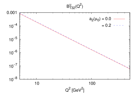
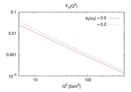
Figure 2: The form factors $B_{T32}^{u}$ and $F_{\pi}$ in collinear factorization, as given in (3.1) and (4). The factorization and renormalization scales are set to $\mu=Q$. The solid (dashed) curve is for $a_{2}=0$ ($0.2$) at $\mu_{0}=2\operatorname{GeV}$, with all other Gegenbauer coefficients set to zero.

Let us now take a look at our result (3.2) for $B_{Tn0}^{u}$. Since the loop integral in (3.2) receives contributions from gluon virtualities ranging all the way from order $Q^{2}$ to order $\Lambda^{2}$, an adequate choice for the renormalization and factorization scales may be to take the geometric mean $\mu^{2}=\Lambda Q$, which we take as a default in the following. In the first panel of Fig. 3 we compare the results obtained with this choice and with the naive choice $\mu^{2}=Q^{2}$. The differences are noticeable but not as large as the ones we discuss next.

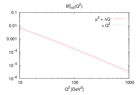
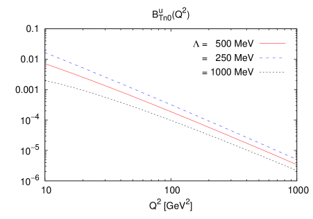
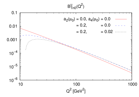
Figure 3: The result (3.2) for the form factor $B_{Tn0}^{u}$. Unless specified in the figure keys, we set the renormalization and factorization scale to $\mu^{2}=\Lambda Q$ with $\Lambda=500\operatorname{MeV}$. As a default we take all Gegenbauer coefficients $a_{n}$ to be zero; the reference scale for nonzero values of $a_{n}$ is $\mu_{0}=2\operatorname{GeV}$.

In the second panel of Fig. 3 we compare the form factor calculated with three different values of the effective parameter $\Lambda$, where the central value $\Lambda=500\operatorname{MeV}$ corresponds to an estimate based on a model of the pion wave function [7], as discussed in the appendix.

In the third panel of the figure we investigate the sensitivity of our result to the twist-two pion distribution amplitude. The difference between the three example choices for the lowest two Gegenbauer coefficients are quite small at high $Q^{2}$ but very noticeable as $Q^{2}$ decreases. We note that the two curves with $a_{2}(\mu_{0})=0.2$ have a zero crossing, which occurs at $Q^{2}=7.8\operatorname{GeV}^{2}$ for $a_{4}(\mu_{0})=0$ and at $Q^{2}=12.2\operatorname{GeV}^{2}$ for $a_{4}(\mu_{0})=0.02$. This behavior can be understood from (3.2). Compared with the term proportional to $\ln^{2}Q/\Lambda$, the contribution linear in $\ln Q/\Lambda$ has a global minus sign and larger numerical coefficients multiplying the $a_{n}$. If $\ln Q/\Lambda$ is not large enough, the linear term can therefore dominate and give a negative result for positive $a_{n}$. As we discussed after (3.2), the strong enhancement of contributions from higher $a_{n}$ is to taken with great caution, and we therefore do not regard the occurrence of a zero crossing for $B_{Tn0}^{u}$ as a reliable prediction.

We note that all curves in Fig. 3 fall less steeply than a pure power law $1/Q^{4}$. This is to be expected since the enhancement by the squared logarithm of $Q^{2}/\Lambda^{2}$ is stronger than the decrease from the scale dependence of $\alpha_{s}(\mu)\,\mu_{\pi}(\mu)\sim\alpha_{s}(\mu)^{\,0.52}$.

Let us finally compare the different form factors for our default choices $\mu^{2}=\Lambda Q$ with $\Lambda=500\operatorname{MeV}$ and $a_{n}=0$. The ratio $B_{Tn0}^{u}/B_{T32}^{u}$ varies between 35 and 240 for $Q^{2}$ between $10$ and $1000\operatorname{GeV}^{2}$. At $Q^{2}=10\operatorname{GeV}^{2}$ we find that $B_{Tn0}^{u}$ is about two thirds of $F_{\pi}$. It is amusing that we obtain $B_{Tn0}^{u}=0.038$ at $Q^{2}=2.5\operatorname{GeV}^{2}$, which is within a factor of a few from the results obtained for $B_{T10}^{u}$ and $B_{T20}^{u}$ in the lattice calculation [2]. This coincidence must, however, not be over-interpreted, given the uncertainties we have just discussed and given that we have not evaluated the $\mathcal{O}(1)$ contribution in (3.2), which is different for different $n$ in $B_{Tn0}^{u}$.

5 Summary

We have studied the tensor form factors of the pion at large squared momentum transfer $Q^{2}$. The matrix element of the chiral-odd quark currents with twist two are written as the convolution of a hard-scattering kernel, the twist-two distribution amplitude for one pion and the twist-three distribution amplitudes for the other pion. In the twist-three sector we take the asymptotic form of the two-particle distribution amplitudes, so that the three-particle distribution amplitudes do not contribute [10, 11].

For the $\xi$-dependent part of the matrix element (2), i.e. for the form factors $B_{Tni}^{u}$ with $i\geq 2$, one can take the collinear limit of the hard-scattering kernel. The result is a representation in standard collinear factorization, in full analogy with the well-known expression (4) for the electromagnetic pion form factor $F_{\pi}$. The form factors $B_{Tni}^{u}$ with $i\geq 2$ behave like $1/Q^{4}$ up to logarithms from the scale dependence of $\alpha_{s}$ and $\mu_{\pi}=m_{\pi}^{2}/(m_{u}+m_{d})$. Numerically, we find that $B_{T32}^{u}$ is more than a factor 10 smaller than $F_{\pi}$ already at $Q^{2}=5\operatorname{GeV}^{2}$.

For the form factors $B_{Tn0}^{u}$ the collinear limit cannot be taken, because the hard-scattering formula then develops logarithmic divergences in the integrations over the longitudinal momentum fraction of the quark in both the incoming and outgoing pion. We have used a simple regularization of the collinear divergences, which involves an effective parameter $\Lambda$ representing the typical transverse momentum in the gluon propagator of the graphs in Fig. 1. The momentum fraction integrals then give enhancement factors $\ln^{2}Q/\Lambda$ and $\ln Q/\Lambda$ that modify the $1/Q^{4}$ power behavior of $B_{Tn0}^{u}$. This is reminiscent of the analysis in [28], where the $1/Q^{6}$ power behavior of the proton Pauli form factor $F_{2}(Q^{2})$ was found to be modified by a squared logarithm $\ln^{2}Q/\Lambda$ related with end-point divergences in a purely collinear calculation.

We have evaluated the logarithmically enhanced terms for $B_{Tn0}^{u}(Q^{2})$ and find that they are independent of the moment index $n$. These terms depend very strongly on the end-point behavior of the twist-two distribution amplitude $\phi(u)$, or equivalently on the Gegenbauer coefficients $a_{n}$ with high $n$. We expect this dependence to be decreased by Sudakov effects, which suppress the end-points at sufficiently large $Q^{2}$. Numerically, we find that for $Q^{2}>10\operatorname{GeV}^{2}$ our approximation of $B_{Tn0}^{u}$ is considerably larger than $B_{Tni}^{u}$ with $i\geq 2$, which is a direct consequence of the enhancement factor $\ln^{2}Q/\Lambda$.

In the present work we have deduced the basic behavior of the form factors $B_{Tni}^{u}$ at large $Q^{2}$. An evaluation that could claim to be quantitatively valid at moderately large $Q^{2}$ would need to use a formalism with a more realistic treatment of the end-point regions in the momentum fractions. Obvious candidates for this are the modified hard-scattering formalism [6, 7, 14, 22] or approaches based on QCD sum rules [5, 8, 9].

Appendix A A simple estimate of $\Lambda$

In order to get some feeling for the typical size of the effective parameter $\Lambda$, let us take a closer look at the replacement of $(\boldsymbol{k}-\boldsymbol{k}^{\prime})^{2}$ by $\Lambda^{2}$ in (38). To this end we assume that $\Sigma(u,k^{2})$ is independent of $u$, so that we can still perform the integrations over $v$ and $u$ as in (3.2) to (3.2). The logarithms $\bigl{[}\ln(Q^{2}/\Lambda^{2})\bigr{]}^{p}$ with $p=1,2$ in (3.2) should then be replaced by

$$\int d^{2}k\,d^{2}k^{\prime}\;\Sigma(k^{2})\,\Sigma(k^{\prime 2})\,\biggl{[}\ln\frac{Q^{2}}{(\boldsymbol{k}-\boldsymbol{k}^{\prime})^{2}}\biggr{]}^{p}.$$ (44)

Let us for simplicity assume a Gaussian form

$$\Sigma(k^{2})=\frac{1}{2\pi\sigma^{2}}\exp\biggl{[}-\frac{\boldsymbol{k}^{2}}{2\sigma^{2}}\biggr{]},$$ (45)

where $\sigma^{2}$ is the average squared transverse momentum in the pion wave function. In a study of $F_{\pi}$ using the modified hard-scattering picture of Li and Sterman, this parameter has been estimated as $\sigma\approx 350\operatorname{MeV}$ in conjunction with the twist-two distribution amplitude $\phi(u)=6u\bar{u}$ [7].

With (45) one can readily perform the integrals (44) after a change of variables from $k$ and $k^{\prime}$ to $k+k^{\prime}$ and $k-k^{\prime}$. The result is

$$\frac{1}{(2\pi)^{2}\mskip 1.5mu\sigma^{4}}\int d^{2}k\,d^{2}k^{\prime}\;\exp\biggl{[}-\frac{\boldsymbol{k}^{2}+\boldsymbol{k}^{\prime 2}}{2\sigma^{2}}\biggr{]}\ln\frac{Q^{2}}{(\boldsymbol{k}-\boldsymbol{k}^{\prime})^{2}}$$

$$\quad=\ln\frac{Q^{2}}{4e^{-\gamma}\mskip 1.5mu\sigma^{2}}\,,$$

$$\frac{1}{(2\pi)^{2}\mskip 1.5mu\sigma^{4}}\int d^{2}k\,d^{2}k^{\prime}\;\exp\biggl{[}-\frac{\boldsymbol{k}^{2}+\boldsymbol{k}^{\prime 2}}{2\sigma^{2}}\biggr{]}\,\biggl{(}\ln\frac{Q^{2}}{(\boldsymbol{k}-\boldsymbol{k}^{\prime})^{2}}\biggr{)}^{2}$$

$$\quad=\biggl{(}\ln\frac{Q^{2}}{4e^{-\gamma}\mskip 1.5mu\sigma^{2}}\biggr{)}^{2}+\frac{\pi^{2}}{6}\,,$$ (46)

where $\gamma=-\int_{0}^{\infty}dx\,e^{-x}\mskip 1.5mu\ln x$ is Euler’s constant. The term $\pi^{2}/6$ can be neglected in our approximation, so that we can consistently identify the first and the second expression in (A) with $\ln(Q^{2}/\Lambda^{2})$ and $\ln^{2}(Q^{2}/\Lambda^{2})$, respectively. We thus find that with the transverse-momentum dependence (45) of the pion wave function we have $\Lambda=2e^{-\gamma/2}\mskip 1.5mu\sigma\approx 1.5\mskip 1.5mu\sigma$, which according to the above estimate for $\sigma$ corresponds to $\Lambda\approx 525\operatorname{MeV}$.

References

• [1] M. Burkardt, Int. J. Mod. Phys.  A 18 (2003) 173 [arXiv:hep-ph/0207047].
• [2] D. Brömmel et al. [QCDSF and UKQCD Collaborations], Phys. Rev. Lett.  101 (2008) 122001 [arXiv:0708.2249 [hep-lat]].
• [3] A. V. Efremov and A. V. Radyushkin, Phys. Lett.  B 94 (1980) 245.
• [4] G. P. Lepage and S. J. Brodsky, Phys. Lett.  B 87 (1979) 359.
• [5] V. A. Nesterenko and A. V. Radyushkin, Phys. Lett.  B 115 (1982) 410.
• [6] H. n. Li and G. Sterman, Nucl. Phys.  B 381 (1992) 129.
• [7] R. Jakob and P. Kroll, Phys. Lett.  B 315 (1993) 463 [Erratum-ibid.  B 319 (1993) 545] [arXiv:hep-ph/9306259].
• [8] V. M. Braun, A. Khodjamirian and M. Maul, Phys. Rev.  D 61 (2000) 073004 [arXiv:hep-ph/9907495].
• [9] A. P. Bakulev, K. Passek-Kumerički, W. Schroers and N. G. Stefanis, Phys. Rev.  D 70 (2004) 033014 [Erratum-ibid.  D 70 (2004) 079906] [arXiv:hep-ph/0405062].
• [10] V. M. Braun and I. E. Filyanov, Z. Phys.  C 48 (1990) 239 [Sov. J. Nucl. Phys.  52 (1990) 126].
• [11] M. Beneke and Th. Feldmann, Nucl. Phys.  B 592 (2001) 3 [arXiv:hep-ph/0008255].
• [12] C. Amsler et al. [Particle Data Group], Phys. Lett.  B 667 (2008) 1.
• [13] M. Beneke, G. Buchalla, M. Neubert and C. T. Sachrajda, Nucl. Phys.  B 606 (2001) 245 [arXiv:hep-ph/0104110].
• [14] S. V. Goloskokov and P. Kroll, Eur. Phys. J.  C 65 (2010) 137 [arXiv:0906.0460 [hep-ph]].
• [15] B. V. Geshkenbein and M. V. Terentev, Phys. Lett.  B 117 (1982) 243.
• [16] B. V. Geshkenbein and M. V. Terentev, Yad. Fiz.  39 (1984) 873. [Sov. J. Nucl. Phys.  39 (1984) 554].
• [17] M. Diehl, A. Manashov and A. Schäfer, Eur. Phys. J.  A 31 (2007) 335 [arXiv:hep-ph/0611101].
• [18] S. Descotes-Genon and C. T. Sachrajda, Nucl. Phys.  B 625 (2002) 239 [arXiv:hep-ph/0109260].
• [19] E. Ruiz Arriola and W. Broniowski, Phys. Rev.  D 66 (2002) 094016 [arXiv:hep-ph/0207266].
• [20] A. V. Radyushkin, Phys. Rev.  D 80 (2009) 094009 [arXiv:0906.0323 [hep-ph]].
• [21] M. V. Polyakov, JETP Lett.  90 (2009) 228 [arXiv:0906.0538 [hep-ph]].
• [22] H. n. Li and S. Mishima, Phys. Rev.  D 80 (2009) 074024 [arXiv:0907.0166 [hep-ph]].
• [23] S. Noguera and V. Vento, arXiv:1001.3075 [hep-ph].
• [24] B. Melić, B. Nižić and K. Passek, Phys. Rev.  D 60 (1999) 074004 [arXiv:hep-ph/9802204].
• [25] S. Bethke, Eur. Phys. J.  C 64 (2009) 689 [arXiv:0908.1135 [hep-ph]].
• [26] V. M. Braun et al. [QCDSF and UKQCD Collaborations], Phys. Rev.  D 74 (2006) 074501 [arXiv:hep-lat/0606012].
• [27] M. A. Donnellan et al. [UKQCD and RBC Collaborations], PoS LAT2007 (2007) 369 [arXiv:0710.0869 [hep-lat]].
• [28] A. V. Belitsky, X. d. Ji and F. Yuan, Phys. Rev. Lett.  91 (2003) 092003 [arXiv:hep-ph/0212351].