THE PROMINENT ROLE OF THE HEAVIEST FRAGMENT IN MULTIFRAGMENTATION AND PHASE TRANSITION FOR HOT NUCLEI
Indra and Aladin Collaborations

Abstract

The role played by the heaviest fragment in partitions of multifragmenting hot nuclei is emphasized. Its size/charge distribution (mean value, fluctuations and shape) gives information on properties of fragmenting nuclei and on the associated phase transition.

1 Introduction

Nuclear multifragmentation was predicted long ago [1] and studied since the early 80’s. The properties of fragments which are issued from the disintegration of hot nuclei are expected to reveal and bring information on a phase transition of the liquid-gas type. Such a phase transition is theoretically predicted for nuclear matter. Nuclear physicists are however dealing with finite systems. Following the concepts of statistical physics, a new definition of phase transitions for such systems was recently proposed, showing that specific phase transition signatures could be expected. [2, 3, 4] Different and coherent signals of phase transition have indeed been evidenced. It is only with the advent of powerful 4$\pi$ detectors [5] like INDRA [6] that real advances were made. With such an array in particular the heaviest fragment of multifragmentation partitions is well identified in charge and its kinetic energy well measured by taking into account pulse-height defect in silicon detectors [7] and effect of the delta-rays in CsI(Tl) scintillators. [8, 9] This paper emphasizes the importance of the heaviest fragment properties in relation with hot fragmenting nuclei (excitation energy and freeze-out volume) and with the associated phase transition of the liquid-gas type (order parameter and generic signal for finite systems).

2 Heaviest fragment and partitions

The static properties of fragments emitted by hot nuclei formed in central (quasi-fused systems (QF) from ${}^{129}Xe$+${}^{nat}Sn$, 25-50 AMeV) and semi-peripheral collisions (quasi-projectiles (QP) from ${}^{197}Au$+${}^{197}Au$, 80 and 100 AMeV) have been compared in detail [10] on the excitation energy domain 4-10 AMeV. To do that hot nuclei showing, to a certain extent, statistical emission features were selected. For central collisions (QF events) one selects complete and compact events in velocity space (constraint of flow angle $\geq 60^{\circ}$). For peripheral collisions (QP subevents) the selection method applied to quasi-projectiles minimizes the contribution of dynamical emissions by imposing a compacity of fragments in velocity space. Excitation energies of the different hot nuclei produced are calculated using the calorimetry procedure (see [10] for details).

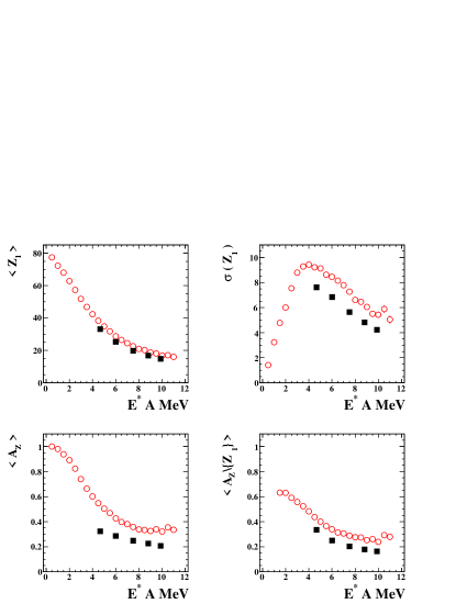
Figure 1: Full squares and open circles stand respectively for QF and QP sources; Top: average values (left) and standard deviation (right) of the charge of the biggest fragment vs the excitation energy per nucleon. Bottom: evolution of the charge asymmetry - with (left) and without (right) the biggest fragment - as a function of the excitation energy per nucleon.

First, it is observed that both the percentage of charge bound in fragments and the percentage of light charged particles participating to the total charged product multiplicity are the same for QF and QP sources with equal excitation energy. Thus such percentages provide a good estimate of the excitation energy of hot nuclei which undergo multifragmentation.

What about the size/charge of the heaviest fragment of partitions, $Z_{1}$ ?

In figure 1 (upper part), the evolutions, with the excitation energy, of its mean value and of the associated fluctuations are plotted. The average charge of the heaviest fragment, for a given system, first strongly decreases with increasing excitation energy and then tends to level off, due to the fixed lowest charge value for fragments. So the mean value appears as also mainly governed by excitation energy and is largely independent of system size and of production modes (see [4] for limitations). This effect was already observed in [11] for two QF sources with charges in the ratio 1.5; its occurrence when comparing QF and QP sources would indicate that their excitation energy scales do agree, within 10%. The fluctuations, on the contrary, exhibit sizeable differences. In the common energy range, the fluctuations of $Z_{1}$ decrease when the excitation energy increases but they are larger for QP sources. In this latter case they show a maximum value around 4 AMeV which is in good agreement with systematics reported for QP sources in [12, 13] and seems to correspond to the center of the spinodal region as defined by the divergences of the microcanonical heat capacity. [14, 15] Differences relative to the fluctuations of $Z_{1}$ for QF and QP sources were also discussed in [13] and a possible explanation was related to different freeze-out volumes by comparison with statistical model (SMM) calculations. We shall see in the next section that indeed different freeze-out volumes have also been estimated from simulations. An overview of all information related to fragment charge partition is obtained with the generalized charge asymmetry variable calculated event by event. [10] To take into account distributions of fragment multiplicities which differ for the two sources, the generalized asymmetry ($A_{Z}$) is introduced: $A_{Z}=\sigma_{Z}/(\langle Z\rangle\sqrt{M_{frag}-1})$. This observable evolves from 1 for asymmetric partitions to 0 for equal size fragment partitions. For the one fragment events, mainly present for QP sources, we compute the $A_{Z}$ observable by taking “as second fragment” the first particle in size hierarchy included in calorimetry. In the left bottom part of fig. 1, the mean evolution with excitation energy of the generalized asymmetry is shown. Differences are observed which well illustrate how different are the repartitions of $Z_{frag}$ between fragments for QF and QP multifragmenting sources. QP partitions are more asymmetric in the entire common excitation energy range. To be sure that this observation does not simply reflect the peculiar behaviour of the biggest fragment, the generalized asymmetry is re-calculated for partitions $M_{frag}>1$, and noted $A_{Z}\backslash\{Z_{1}\}$, by removing $Z_{1}$ from partitions (bottom right panel of fig. 1). The difference between the asymmetry values for the two source types persists.

3 Heaviest fragment and freeze-out volume

Starting from all the available experimental information of selected QF sources produced in central ¹²⁹Xe+^natSn collisions which undergo multifragmentation, a simulation was performed to reconstruct freeze-out properties event by event. [16, 17] The method requires data with a very high degree of completeness, which is crucial for a good estimate of Coulomb energy. The parameters of the simulation were fixed in a consistent way including experimental partitions, kinetic properties and the related calorimetry. The necessity of introducing a limiting temperature related to the vanishing of level density for fragments [18] in the simulation was confirmed for all incident energies. This naturally leads to a limitation of their excitation energy around 3.0-3.5 AMeV as observed in. [19]

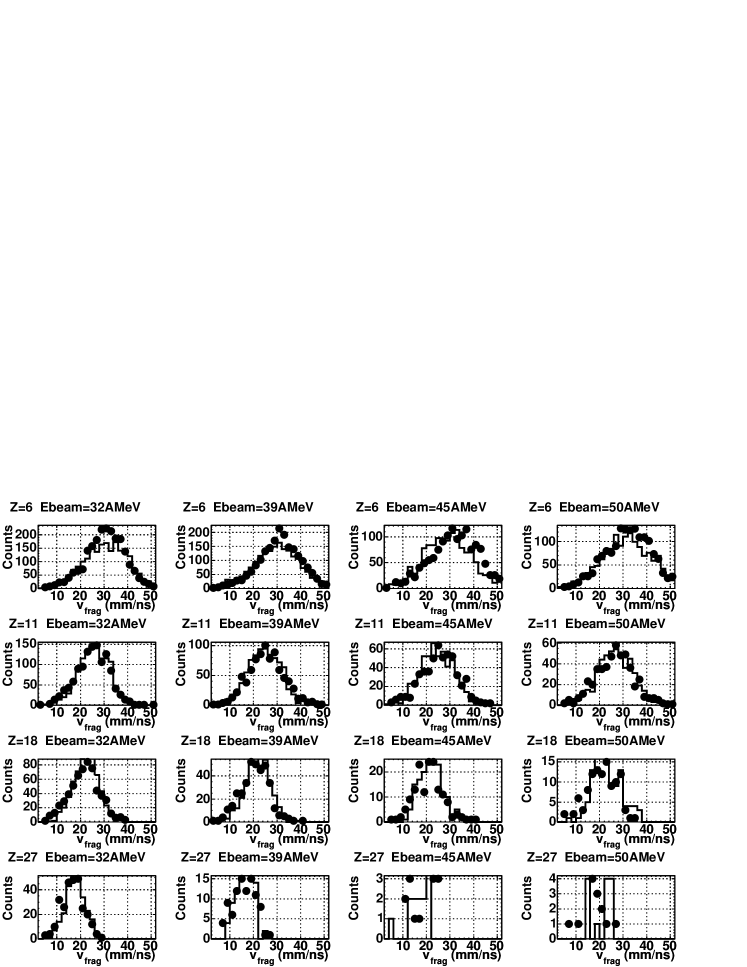
Figure 2: Comparison between the experimental velocity spectra (full points) of fragments of a given charge and the simulated ones (histograms). Each row refers to a different fragment charge: starting from the top $Z=6$, $Z=11$, $Z=18$, $Z=27$. Each column refers to a different beam energy: starting from the left 32 AMeV, 39 AMeV, 45 AMeV and 50 AMeV. From. [17]

The experimental and simulated velocity spectra for fragments of given charges (Z=6, 11, 18 and 27) are compared in fig. 2 for the different beam energies; when the statistics are sufficient the agreement is quite remarkable. Finally relative velocities between fragment pairs were also compared through reduced relative velocity correlation functions [20, 21, 22, 23] (see fig. 3).

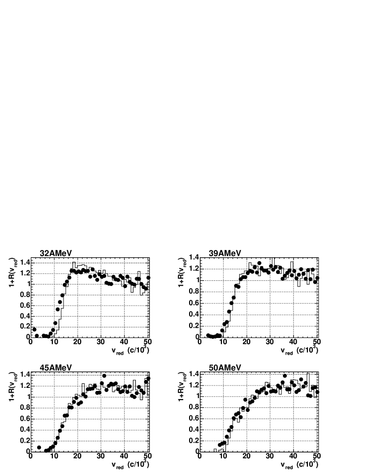
Figure 3: Comparison between the experimental (full points) and simulated (histograms) reduced relative velocity correlation functions for all the fragments. The reduced relative velocity between two fragments with charges $Z_{i}$ and $Z_{j}$ ($Z_{i,j}>$4) is defined as $v_{red}$=$v_{rel}$/$(Z_{i}+Z_{j})^{1/2}$. Each panel refers to a different beam energy: 32 AMeV (top left), 39 AMeV (top right), 45 AMeV (bottom left) and 50 AMeV (bottom right). From. [17]

In the simulation the fragment emission time is by definition equal to zero and correlation functions are consequently only sensitive to the spatial arrangement of fragments at break-up and the radial collective energy involved (hole at low reduced relative velocity), to source sizes/charges and to excitation energy of the sources (more or less pronounced bump at $v_{red}$= 0.02-0.03c). Again a reasonable agreement is obtained between experimental data and simulations, especially at 39 and 45 AMeV incident energies, which indicates that the retained method and parameters are sufficiently relevant to correctly describe freeze-out topologies and properties.

The major properties of the freeze-out configurations thus derived are the following: an important increase, from $\sim$20% to $\sim$60%, of the percentage of particles present at freeze-out between 32 and 45-50 AMeV incident energies accompanied by a weak increase of the freeze-out volume which tends to saturate at high excitation energy. Finally, to check the overall physical coherence of the developed approach, a detailed comparison with a microcanonical statistical model (MMM) was done. The degree of agreement, which was found acceptable, confirms the main results and gives confidence in using those reconstructed freeze-out events for further studies as it is done in. [10]

Estimates of freeze-out volumes for QF sources produced in Xe+Sn collisions for incident energies between 32 and 50 AMeV evolve from 3.9 to 5.7 $V/V_{0}$, where $V_{0}$ would correspond to the volume of the source at normal density. [17]

To calibrate the freeze-out volumes for other sources, we use the charge of the heaviest fragment $<Z_{1}^{(N)}>$ or the fragment multiplicity $<M_{frag}^{(N)}>$, normalized to the size of the source, as representative of the volume or density at break-up. From the four points for QF sources and the additional constraint that $Z_{1}^{(N)}=M_{frag}$=1 at $V/V_{0}$=1, we obtain two relations $V/V_{0}=f_{1}(Z_{1}^{(N)})$ and $V/V_{0}=f_{2}(M_{frag}^{(N)})$, from which we calculate the volumes for QF sources at 25 AMeV and for QP sources. The results are plotted in fig. 4, with error bars coming from the difference between the two estimates using $f_{1}$ and $f_{2}$; note that error bars for the QP volumes are small up to 7 AMeV, and can not be estimated above, due to the fall of $<M_{frag}^{(N)}>$ at high energy (see fig. 5 of [10]). So only $<(Z_{1}^{(N)}>)$ can be used over the whole excitation energy range considered and the derived function is the following:
$V/V_{0}=exp(2.47-4.47<(Z_{1}^{(N)}>)+0.86$.

The volumes of QP sources are smaller than those of QF sources (by about 20% on the $E^{*}$ range 5-10 AMeV). This supports the explanation discussed previously starting from fluctuations of the charge of the heaviest fragment in a partition.

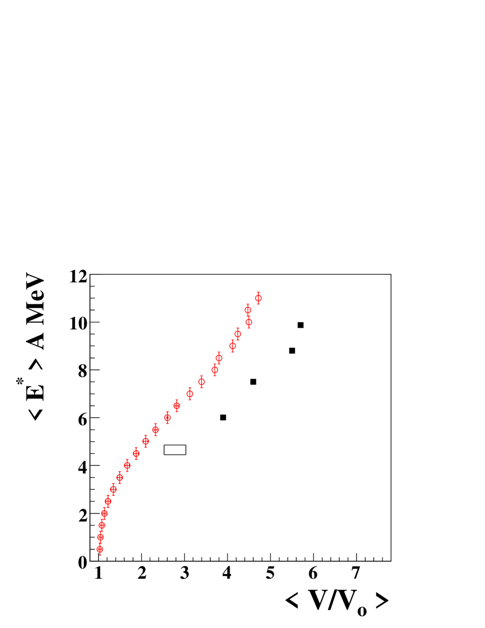
Figure 4: Fragmentation position in the excitation energy-freeze-out volume plane. The four full squares (QF sources) are taken from [17]. The open rectangle gives the estimated position (with error bar) for QF source at 25 AMeV, and the open circles those for QP sources. From. [10]

$Z_{1}$ also presents some specific dynamical properties. As shown in [24, 23] for QF sources, its average kinetic energy is smaller than that of other fragments with the same charge. The effect was observed whatever the fragment multiplicity for Xe+Sn between 32 and 50 AMeV and for Gd+U at 36 AMeV. The fragment-fragment correlation functions are also different when one of the two fragments is $Z_{1}$. This observation was connected to the event topology at freeze-out, the heavier fragments being systematically closer to the centre of mass than the others.

4 Heaviest fragment and order parameter

The recently developed theory of universal scaling laws of order-parameter fluctuations provides methods to select order parameters. [25, 26] In this framework, universal $\Delta$ scaling laws of one of the order parameters, $m$, should be observed:
$\langle m\rangle^{\Delta}P(m)=\phi((m-\langle m\rangle)/\langle m\rangle^{\Delta})$
where $\langle m\rangle$ is the mean value of the distribution $P(m)$. $\Delta$=1/2 corresponds to small fluctuations, $\sigma_{m}^{2}\sim\langle m\rangle$, and thus to an ordered phase. Conversely $\Delta$=1 occurs for the largest fluctuations nature provides, $\sigma_{m}^{2}\sim\langle m\rangle^{2}$, in a disordered phase. For models of cluster production there are two possible order parameters: [26] the fragment multiplicity in a fragmentation process or the size of the largest fragment in an aggregation process (clusters are built up from smaller constituents). The method was applied to central collision samples (symmetric systems with total masses $\sim$73-400 at bombarding energies between 25 and 100 AMeV) .[27, 28] The total (charged products) or fragment multiplicity fluctuations do not show any evolution over the whole data set. Conversely the relationship between the mean value and the fluctuation of the size of the largest fragment does change as a function of the bombarding energy: $\Delta\sim$1/2 at low energy, and $\Delta\sim$1 for higher bombarding energies. The form of the $Z_{max}$ distributions also evolves with bombarding energy: it is nearly Gaussian in the $\Delta$=1/2 regime and exhibits for $\Delta$=1 an asymmetric form with a near-exponential tail for large values of the scaling variable (see fig. 5). This distribution is close to that of the modified Gumbel distribution, [29] the resemblance increasing with the total mass of the system studied and being nearly perfect for the Au+Au data. The Gumbel distribution is the equivalent of the Gaussian distribution in the case of extreme values: it is obtained for an observable which is an extremum of a large number of random, uncorrelated, microscopic variables.

file=fig5_IWNDborderie.eps,width=9cm

Figure 5: (a) $Z_{max}$ distributions for central Xe+Sn collisions at 25-39 AMeV bombarding energies, scaled according to $\Delta$ scaling equation; the dashed curve is a best fit to scaled data using a Gaussian distribution. (b) As (a) but for bombarding energies 39-100 AMeV: the dashed curve is a best fit to scaled data using the Gumbel distribution. From. [27]

Within the developed theory, this behaviour indicates, for extensive systems, the transition from an ordered phase to a disordered phase in the critical region, the fragments being produced following some aggregation scenario. However simulations for finite systems have been performed in the framework of the Ising model [30] which show that the distribution of the heaviest fragment approximately obeys the $\Delta$=1 scaling regime even at subcritical densities where no continuous transition takes place. The observed behaviour was interpreted as a finite size effect that prevents the recognition of the order of a transition in a small system. More recently the distribution of the heaviest fragment was analyzed within the lattice gas model [31] and it was shown that the most important finite size effect comes from conservation laws, the distribution of the order parameter being strongly deformed if a constraint is applied (mass conservation) to an observable that is closely correlated to the order parameter. Moreover the observation of the $\Delta$=1 scaling regime was indeed observed in the critical zone but was also confirmed at subcritical densities inside the coexistence region.

5 Heaviest fragment and first order phase transition

At a first-order phase transition, the distribution of the order parameter in a finite system presents a characteristic bimodal behavior in the canonical or grandcanonical ensemble. [32, 33, 34, 35] The bimodality comes from an anomalous convexity of the underlying microcanonical entropy. [36] It physically corresponds to the simultaneous presence of two different classes of physical states for the same value of the control parameter, and can survive at the thermodynamic limit in a large class of physical systems subject to long-range interactions. [37]

Indeed if one considers a finite system in contact with a reservoir (canonical sampling), the value of the extensive variable (order parameter) X may fluctuate as the system explores the phase space. The entropy function F(X) is no more addititive due to the fact that surfaces are not negligible for finite systems and the resulting equilibrium entropy function has a local convexity. The Maxwell construction is no longer valid. The associated distribution at equilibrium is $P(X)$$\sim$exp($S(X)$-$\lambda X$) where $\lambda$ is the corresponding Lagrange multiplier. The distribution of $X$ acquires a bimodal character (see fig. 6).

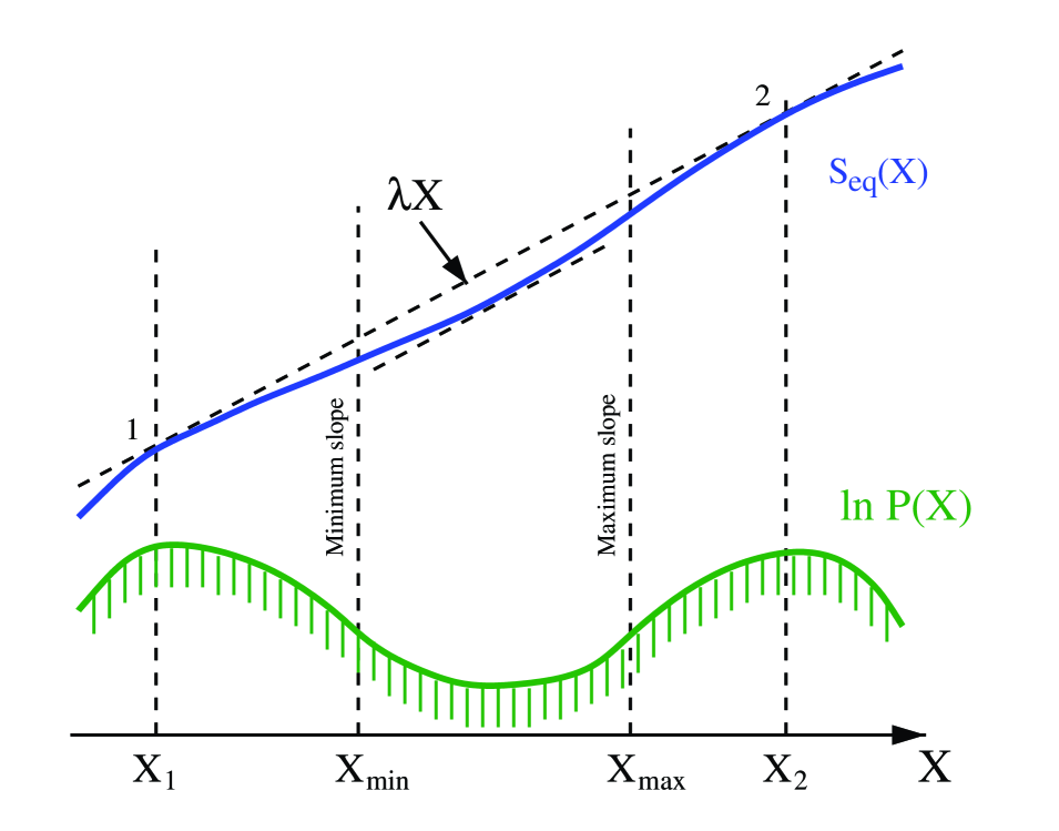
Figure 6: Canonical ensemble of finite systems. The bimodal equilibrium distribution is given by $P(X)$$\sim$exp($S(X)$-$\lambda X$). The figure shows the case when the Lagrange multiplier $\lambda$ is equal to the slope of the common tangent (from [38]).

In the case of nuclear multifragmentation, we have shown in the previous section that the size of the heaviest cluster produced in each collision event is an order parameter. A difficulty comes however from the absence of a true canonical sorting in the data. The statistical ensembles produced by selecting for example fused systems are neither canonical nor microcanonical and should be better described in terms of the Gaussian ensemble, [39] which gives a continuous interpolation between canonical and microcanonical ensembles. Recently a simple weighting of the probabilities associated to each excitation energy bin for quasi-projectile events was proposed to allow the comparison with the canonical ensemble. [40] That weighting procedure is used to allow a comparison with canonical expectations for QP sources produced in Au + Au collisions at incident energies from 60 to 100 AMeV. Then, a double saddle-point approximation is applied to extract from the measured data equivalent-canonical distributions. [40]

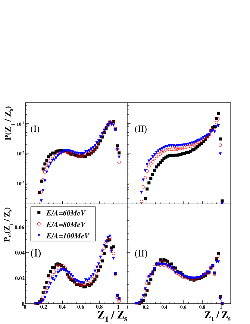
Figure 7: Upper part: measured distribution of the charge of the largest fragment normalized to the charge of the source detected in Au+Au collisions at three different bombarding energies. Lower part: weighted distributions obtained considering the same statistics for each excitation energy bin. The left (right) side shows distributions obtained with the data selection method (I) ((II)). From. [41]

In this incident energy regime, a part of the cross section corresponds to collisions with dynamical neck formation [42]. We thus need to make sure that the observed change in the fragmentation pattern [43] is not trivially due to a change in the size of the QP. After a shape analysis in the center of mass frame [44], only events with a total forward detected charge larger than 80% of the Au charge were considered (quasi-complete subevents). Two different procedures aiming at selecting events with negligible neck contribution were adopted. In the first one [43] (I) by eliminating events where the entrance channel dynamics induces a forward emission, in the quasi-projectile frame, of the heaviest fragment $Z_{1}$. [45] For isotropically decaying QPs, this procedure does not bias the event sample but only reduces the statistics. In a second strategy (II) the reduction of the neck contribution is obtained by keeping only “compact” events by imposing (i) an upper limit on the relative velocity among fragments, and (ii) a QP size constant within 10% (see [10] for details). In both cases fission events were removed. [43]

The results obtained with the two different selection methods are given in fig. 7. To take into account the small variations of the source size, the charge of the heaviest fragment $Z_{1}$ has been normalized to the source size. After the weighting procedure (lower part of the figure), a bimodal behavior of the largest fragment charge clearly emerges in both cases. In particular in the case of selection (II), we can see that the weight of the low $Z_{1}$ component, associated to more fragmented configurations and higher deposited energy, increases with the bombarding energy before the weighting procedure (upper part of the figure). This difference completely disappears when data are weighted, showing the validity of the phase-space dominance hypothesis.

Those weighted experimental distributions can be fitted with an analytic function (see [41] for more details). From the obtained parameter values one can estimate the latent heat of the transition of the hot heavy nuclei studied (Z$\sim$70) as $\Delta E=8.1(\pm 0.4)_{stat}(+1.2-0.9)_{syst}$ AMeV. Statistical error was derived from experimental statistics and systematic errors from the comparison between the two different QP selections.

References

- [1] N. Bohr, Nature 137 (1936) 351.
- [2] B. Borderie, J. Phys. G: Nucl. Part. Phys. 28 (2002) R217.
- [3] P. Chomaz et al. (eds.) vol. 30 of Eur. Phys. J. A, Springer, 2006.
- [4] B. Borderie and M. F. Rivet, Prog. Part. Nucl. Phys. 61 (2008) 551.
- [5] R. T. de Souza et al., P. Chomaz et al. (eds.) Dynamics and Thermodynamics with nuclear degrees of freedom, Springer, 2006, vol. 30 of Eur. Phys. J. A, 275–291.
- [6] J. Pouthas et al., Nucl. Instr. and Meth. in Phys. Res. A 357 (1995) 418.
- [7] G. Tăbăcaru et al. (INDRA Collaboration), Nucl. Instr. and Meth. in Phys. Res. A 428 (1999) 379.
- [8] M. Pârlog et al. (INDRA Collaboration), Nucl. Instr. and Meth. in Phys. Res. A 482 (2002) 674.
- [9] M. Pârlog et al. (INDRA Collaboration), Nucl. Instr. and Meth. in Phys. Res. A 482 (2002) 693.
- [10] E. Bonnet et al. (INDRA and ALADIN Collaborations), Nucl. Phys. A 816 (2009) 1.
- [11] M. F. Rivet et al. (INDRA Collaboration), Phys. Lett. B 430 (1998) 217.
- [12] F. Gulminelli et al., P. Chomaz et al. (eds.) Dynamics and Thermodynamics with nuclear degrees of freedom, Springer, 2006, vol. 30 of Eur. Phys. J. A, 253–262.
- [13] N. Le Neindre et al. (INDRA and ALADIN collaborations), Nucl. Phys. A 795 (2007) 47.
- [14] M. D’Agostino et al., Nucl. Phys. A 734 (2004) 512.
- [15] E. Bonnet, thèse de doctorat, Université Paris-XI Orsay (2006), http://tel.archives-ouvertes.fr/tel-00121736.
- [16] S. Piantelli et al. (INDRA Collaboration), Phys. Lett. B 627 (2005) 18.
- [17] S. Piantelli et al. (INDRA Collaboration), Nucl. Phys. A 809 (2008) 111.
- [18] S. E. Koonin and J. Randrup, Nucl. Phys. A 474 (1987) 173.
- [19] S. Hudan et al. (INDRA Collaboration), Phys. Rev. C 67 (2003) 064613.
- [20] Y. D. Kim et al., Phys. Rev. C 45 (1992) 338.
- [21] D. R. Bowman et al., Phys. Rev. C 52 (1995) 818.
- [22] D. H. E. Gross, Phys. Rep. 279 (1997) 119.
- [23] G. Tăbăcaru et al. (INDRA Collaboration), Nucl. Phys. A 764 (2006) 371.
- [24] N. Marie et al. (INDRA Collaboration), Phys. Lett. B 391 (1997) 15.
- [25] R. Botet et al., Phys. Rev. E 62 (2000) 1825.
- [26] R. Botet et al., Universal fluctuations, World Scientific, 2002, vol. 65 of World scientific Lecture Notes in Physics.
- [27] J. D. Frankland et al. (INDRA and ALADIN collaborations), Phys. Rev. C 71 (2005) 034607.
- [28] R. Botet et al., Phys. Rev. Lett. 86 (2001) 3514.
- [29] E. J. Gumbel, Statistics of extremes, Columbia University Press, 1958.
- [30] J. M. Carmona et al., Phys. Lett. B 531 (2002) 71.
- [31] F. Gulminelli et al., Phys. Rev. C 71 (2005) 054607.
- [32] K. Binder et al., Phys. Rev. B 30 (1984) 1477.
- [33] P. Chomaz et al., Phys. Rev. E 64 (2001) 046114.
- [34] P. Chomaz et al., Physica A 330 (2003) 451.
- [35] F. Gulminelli, Ann. Phys. Fr. 29 (2004) No 6.
- [36] D. H. E. Gross, Microcanonical thermodynamics, World Scientific, 2002, vol. 66 of World scientific Lecture Notes in Physics.
- [37] T. Dauxois et al. (eds.) vol. 602 of Lecture Notes in Physics, Springer-Verlag, Heidelberg, 2002.
- [38] P. Chomaz et al., Phys. Rep. 389 (2004) 263.
- [39] M. Challa et al., Phys. Rev. Lett. 60 (1988) 77.
- [40] F. Gulminelli, Nucl. Phys. A 791 (2007) 165.
- [41] E.Bonnet et al. (INDRA Collaboration), Phys. Rev. Lett. 103 (2009) 072701.
- [42] M. D. Toro et al., P. Chomaz et al. (eds.) Dynamics and Thermodynamics with nuclear degrees of freedom, Springer, 2006, vol. 30 of Eur. Phys. J. A, 65–70.
- [43] M. Pichon et al. (INDRA and ALADIN collaborations), Nucl. Phys. A 779 (2006) 267.
- [44] D. Cugnon et al., Nucl. Phys. A 397 (1983) 519.
- [45] J. Colin et al. (INDRA Collaboration), Phys. Rev. C 67 (2003) 064603.