Cosmological parameters from large scale structure - geometric versus shape information
Abstract:
The matter power spectrum as derived from large scale structure (LSS) surveys contains two important and distinct pieces of information: an overall smooth shape and the imprint of baryon acoustic oscillations (BAO). We investigate the separate impact of these two types of information on cosmological parameter estimation for current data, and show that for the simplest cosmological models, the broad-band shape information currently contained in the SDSS DR7 halo power spectrum (HPS) is by far superseded by geometric information derived from the baryonic features. An immediate corollary is that contrary to popular beliefs, the upper limit on the neutrino mass presently derived from LSS combined with cosmic microwave background (CMB) data does not in fact arise from the possible small-scale power suppression due to neutrino free-streaming, if we limit the model framework to minimal CDM+. However, in more complicated models, such as those extended with extra light degrees of freedom and a dark energy equation of state parameter differing from , shape information becomes crucial for the resolution of parameter degeneracies. This conclusion will remain true even when data from the Planck spacecraft are combined with SDSS DR7 data. In the course of our analysis, we update both the BAO likelihood function by including an exact numerical calculation of the time of decoupling, as well as the HPS likelihood, by introducing a new dewiggling procedure that generalises the previous approach to models with an arbitrary sound horizon at decoupling. These changes allow a consistent application of the BAO and HPS data sets to a much wider class of models, including the ones considered in this work. All the cases considered here are compatible with the conservative 95%-bounds , .
1 Introduction
Our best source of information about cosmological parameters at present is the precision measurement of the cosmic microwave background (CMB) anisotropies by the Wilkinson Microwave Anisotropy Probe (WMAP) [1]. However, except in the simplest models, the CMB on its own does not provide very tight constraints on specific model parameters because of parameter degeneracies. One very well known example is the bound on neutrino masses, which in the simplest vanilla+ model can be significantly improved by adding information extracted from surveys of the large scale structure (LSS) distribution. Moreover, if the model space is extended, degeneracies with other parameters such as the dark energy equation of state parameter quickly deteriorate the neutrino mass bound from CMB data alone. In such cases it is necessary to appeal to other cosmological probes (e.g., LSS, Type Ia supernovæ) in order to alleviate the degeneracies.
In many recent analyses (e.g., [1]), the only information from LSS surveys employed in the parameter estimation pipeline is the length scale associated with the baryon acoustic oscillation (BAO) peak in the two-point correlation function. We call this geometric information, since a known and measured length scale (a “standard ruler”) allows for the determination of the angular diameter distance to the object of interest simply via geometric effects. The common view is that the BAO length scale is a more robust observable than the broad-band shape of the power spectrum which may suffer from ill-understood nonlinear effects, such as nonlinear clustering or redshift- and scale-dependent galaxy/halo bias.111The turning point of the matter power spectrum in space corresponds to the comoving Hubble radius at the time of matter-radiation equality and in principle also constitutes a geometric measure. However, since this length scale has yet to be measured, we prefer to consider the turning point as part of the broad-band shape of the power spectrum. Indeed, two recent studies of cosmological parameter constraints from combining CMB information with either the BAO scale from SDSS alone [2], or including both the broad-band shape of the SDSS DR7 halo power spectrum and BAO information [3] find very similar parameter estimates and uncertainties for the simplest vanilla model. Somewhat surprisingly, the same conclusion holds also when the vanilla model is extended with a finite neutrino mass which should in principle be very sensitive to the broad-band shape. Thus circumstantial evidence seems to suggest that in the simplest cosmological models, geometric information from the BAO wiggles supersedes the information contained in the broad-band shape of the matter power spectrum.
However, as we shall demonstrate, for more complicated models the additional information contained in the broad-band shape of the matter power spectrum can make a very substantial difference to parameter inference . For example, in models where the number of relativistic degrees of freedom and the dark energy equation of state parameter are added as free parameters, the difference in the parameter uncertainties between including and excluding the power spectrum shape information can be a factor of two or more (see also Ref. [4] for a related discussion in the context of CMB data and dark energy models).
The purpose of the present work is to clarify the roles of “geometric” and “shape” information extractable from the current generation of LSS surveys, and to stress that in extended models geometric information alone does not optimally exploit the available data. This will remain true even when CMB data from the Planck spacecraft become available. The paper is organised as follows: In section 2 we describe the specific cosmological parameter space used, the data sets, as well as the analysis method. We present our results in section 3, including a forecast for Planck. Our conclusions can be found in section 4. Appendices A and B contain details of our methodology.
2 Analysis
2.1 Models
We consider extensions of the minimal cosmological (vanilla) model, characterised by the free parameters listed in Table 1. Flat priors are used on all parameters.222 Note that here, represents the number of massive neutrinos sharing a common mass , while the neutrino fraction is defined as with and . This parameterisation of the neutrino sector is not very realistic from the particle physics point of view. A better parameterisation might assign a free parameter to denote exclusively massless particle species, another parameter for massive species, and . However, the difference between the cosmological signatures of these various models is small given the sensitivity of the data, and introducing massive neutrinos (i.e., setting and ) as we do here makes for a much simpler analysis.
| Parameter | Symbol | Prior range |
|---|---|---|
| Baryon density | ||
| Dark matter density | ||
| Hubble parameter | ||
| Reionisation optical depth | ||
| Amplitude of scalar spectrum @ | ||
| Scalar spectral index | ||
| Neutrino fraction | ||
| Effective number of radiation degrees of freedom | ||
| Dark energy equation of state parameter |
2.2 Data
Our main focus in this work is the halo power spectrum (HPS) constructed from the luminous red galaxy sample of the seventh data release of the Sloan Digital Sky Survey (SDSS-DR7) [3]. The full HPS data set consists of 45 data points, covering wavenumbers from to (where and denote the wavenumber at which the the window functions of the first and last data point have their maximum). We shall use several subsets of the full HPS data, taking into account only the first data points (where is a natural number ranging from 1 to 9) – this corresponds to a short-scale cutoff between and , in steps of .
Our goal is to disentangle the effects of shape and geometrical information on cosmological parameter constraints. To this end we perform the following parameter fits:
-
1.
We fit the HPS of Ref. [3] as per usual, using a properly smeared power spectrum to model nonlinear mode-coupling. The smearing procedure requires that we supply a smooth, featureless (no-wiggle) power spectrum, which we construct using a new discrete spectral analysis technique (in contrast to the interpolation method used in Refs. [3, 5], which is, strictly speaking, not applicable in extended cosmological models). See Appendix A for details. The result of this fit will contain both shape and geometric information.
-
2.
We fit the no-wiggle spectrum alone to Reid et al.’s HPS data. This fit singles out the broad-band shape information.
-
3.
We use the the measurement of the baryon acoustic oscillation (BAO) scale obtained from SDSS-DR7 [2], which represents solely the geometric information contained in the galaxy survey data. Since the acoustic scale depends in principle on such parameters as , care needs to be taken when evaluating the BAO likelihood. We refer the reader to Appendix B for details.
Since large scale structure data by themselves are not able to break all the parameter degeneracies of our cosmological models, we complement the power spectrum/BAO data with a compilation of measurements of the CMB temperature and polarisation anisotropies, consisting of WMAP 7-year [6], ACBAR [7], BICEP [8] and QuAD [9] data, as well as the HST constraint on the Hubble parameter [10]. We avoid redundancies between the CMB data sets in the same way as in Ref. [11].
We employ a modified version of the Markov-chain Monte Carlo code CosmoMC [12] to construct the posterior probability density of the free model parameters. For each combination of model and data, we generate eight chains in parallel and monitor convergence with the Gelman-Rubin -parameter [13], imposing a conservative convergence criterion of .
3 Results
3.1 Vanilla++,
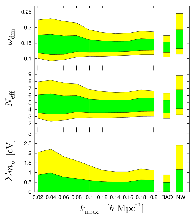
Let us assume the dark energy to be a cosmological constant for now. In Figure 1 we plot the constraints on the cosmological parameters that benefit the most from the addition of LSS data to our basic CMB+HST data set (, and ) as a function of . These results give rise to the following observations:
-
1.
There is no significant trend in the parameter estimates as smaller scale data are added, which implies a reassuring absence of obvious inconsistencies between the cosmological model and the HPS likelihood.
-
2.
The greatest improvement in parameter constraints is apparent around . This is consistent with the fact that the BAO bump in the correlation function is around [14]. Hence one requires to observe a full oscillation in the power spectrum in order to be sensitive to the geometric information contained in the BAO scale.
-
3.
Adding data points beyond does not lead to any further improvement in the parameter constraints. This effect can be attributed to the modelling of nonlinear effects on the spectrum. First, the onset of smoothing of the BAO due to mode coupling at , which limits the amount of information that can be gained about the BAO scale at large , and second, the marginalisation procedure that is meant to model residual uncertainties in the nonlinear distortions of the spectrum, which obscures any shape information contained in the large- power spectrum.
-
4.
Parameter constraints from a fit of a featureless no-wiggle spectrum to the full HPS data which ignores any geometrical information do not show any improvement over those derived from an analysis without large scale structure data.
-
5.
The BAO data lead to slightly tighter bounds on the parameters than the HPS data (see Table 2). Along with point 4., this implies that the shape information does not contribute any relevant additional information in this model.
The fact that BAO slightly outperforms HPS may seem somewhat surprising at first glance, but there are several reasons that could account for this phenomenon. First, the BAO data make use of the full SDSS galaxy sample instead of just the LRGs. Second, the BAO data constrains the BAO scale at two distinct redshifts, whereas the HPS data as implemented at the moment only constrain the BAO scale at one effective distance obtained from averaging over the mean redshifts of the FAR, MID and NEAR LRG-subsamples. Additionally, since the geometric information is obtained through different analysis pipelines, we cannot rule out the possibility that one of them may be slightly more aggressive and thus yield tighter constraints.
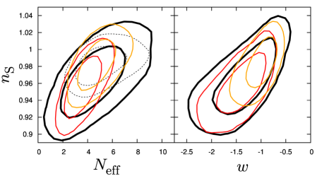
On a side note, it is interesting to point out that due to a parameter degeneracy between and in this model the favoured value for the spectral index is shifted to bluer tilts than in the basic six-parameter vanilla model, with (@ 68% c.l.) for CMB+HST+HPS. In other words, if , the scale-invariant Harrison-Zel’dovich spectrum becomes viable again, with corresponding to (see the thin dotted black contour in the left panel of Figure 2). Even though this would indicate a non-standard cosmology, perhaps with a large amount of late-time entropy production, it does show that with current data the inference that is not completely robust.
3.2 Vanilla+++
Allowing the dark energy equation of state parameter to vary introduces another direction which contributes to the geometric degeneracy. Consequently, one can expect a degradation in parameter constraints compared to the case considered in the previous subsection. The parameter most affected by this turns out to be the spectral index, which is illustrated by the difference between the thick black and thin dotted black contours in Figure 2. The closer is to zero, the more power at large angular scales in the CMB temperature spectrum will be generated due to the late integrated Sachs-Wolfe effect. This, in turn, can be offset to fit present CMB data by removing large-scale primordial power, i.e., going to a bluer spectral index.
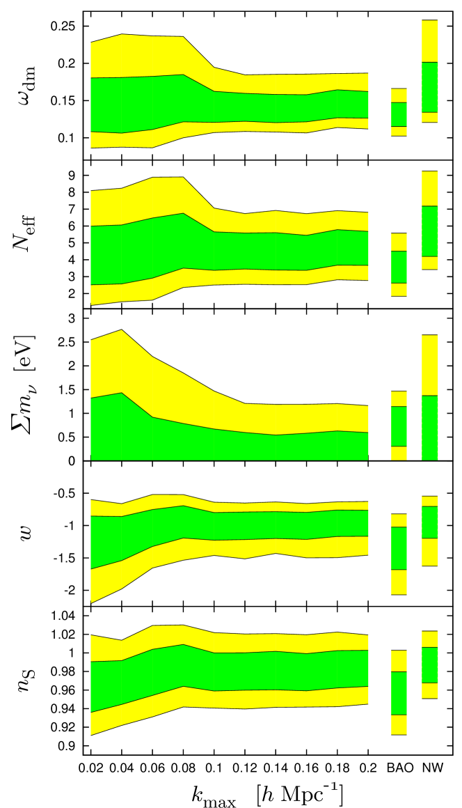
From Figure 3 it can be seen that the internal consistency of the HPS and the sharp improvement in errors around are still present. Notably though, the BAO data alone are not able to break the (,,)-degeneracy present in the basic CMB+HST data. Indeed, BAO are not sensitive to the spectral index. In the previous model with , was reasonably well constrained by the CMB data alone.
In the model at hand though, the CMB cannot resolve the (,)-degeneracy. In order to break it, it becomes crucial to include the shape information of the HPS spectrum. This conclusion is supported by the observation that a fit of the no-wiggle spectrum to HPS data yields essentially the same bounds on and as the usual fit with full HPS data. On the other hand, the best constraints on parameters like still come from the geometric rather than shape information. So, a fit of the full HPS data is necessary in order to get efficient constraints on this model.
| Model | Data set | |||
|---|---|---|---|---|
| CMB+HST | – | |||
| vanilla++ | CMB+HST+BAO | – | ||
| CMB+HST+HPS | – | |||
| CMB+HST | ||||
| vanilla+++ | CMB+HST+BAO | |||
| CMB+HST+HPS |
3.3 A forecast for Planck
| Planck | P+BAO | P+HPS | P+HST | P+HST+BAO | P+HST+HPS | |
|---|---|---|---|---|---|---|
| 0.22 | 0.24 | 0.20 | 0.21 | 0.21 | 0.19 | |
| 0.21 | 0.21 | 0.22 | 0.21 | 0.21 | 0.22 | |
| 0.68 | 0.81 | 0.44 | 0.67 | 0.73 | 0.44 | |
| 2.14 | 1.16 | 0.72 | 0.74 | 0.76 | 0.55 | |
| 0.46 | 0.48 | 0.49 | 0.46 | 0.48 | 0.48 |
The conclusions one can draw about the usefulness of geometric and shape information obviously depend not only on the large scale structure data themselves, but also on the constraining power of the “auxiliary” data used in the analysis. It is thus interesting to ask whether one can expect any qualitative changes from improved future cosmological measurements for the vanilla+++ model. As an example we consider a forecast of simulated fiducial temperature and polarisation data from the Planck spacecraft [16] using the method of Ref. [17]. Our results in Table 3 show that Planck data alone will suffice to constrain , and . Nonetheless, the bounds on neutrino mass and will still profit from the addition of large scale structure data – and significantly, the SDSS shape information will remain important.
4 Conclusions
We have studied in detail how various subsets of the power spectrum information from a large scale structure survey can be used to constrain cosmological parameters. At present an often used approach is to restrict the LSS information to the geometric distance information contained in the BAO peak. For the minimal CDM model (with neutrino mass included) this does indeed provide exactly the same constraint as the use of the full power spectrum data, and is far superior to using a smoothed no-wiggle power spectrum which contains only shape information. This indicates that the neutrino mass is currently more strongly constrained by its effect on the background evolution [18], and the contribution of present LSS data consists mainly in alleviating the geometrical degeneracy with and [19, 20], rather than constraining the possible small-scale power suppression in the large scale matter power spectrum due to free-streaming.
However, this simple picture changes when more complex cosmological models are studied.333We should point out a small caveat here: the usefulness of the LSS shape information depends not only on the cosmological model under consideration, but also on the combination of data sets used in the analysis. For example, Reid et al. [3] find that in a vanilla+ model, WMAP5+HPS yields much better constraints on than WMAP5+BAO. However, in this model the LSS shape information loses its usefulness as soon as one adds the HST constraint, which breaks the (-)-degeneracy more efficiently – leading to conclusions similar to those found in our subsection 3.1. As an example we have tested a model with a variable number of neutrino species, and a dark energy equation of state, , different from -1. In this model some parameters are still as well constrained by BAO alone as by the full power spectrum. This is true for example for the number of neutrino species, which is mainly probed by CMB data, and the dark matter density which is highly sensitive to the position of the BAO peak. However, for other parameters such as , and , there is additional information in the shape of the power spectrum which is crucial for constraining these parameters. For example the upper 95% bound on neutrino mass goes from to when BAO information is replaced with the full halo power spectrum.
However, even in this model, the entire shape information of the HPS is contained in the data points at wavenumbers smaller than , the higher- information being diluted due to uncertainties in nonlinear modelling. In other words, due to our ignorance of the processes governing the power spectrum at smaller scales, we basically lose almost half of the available data points (the half that is less subject to sample variance at that!). Clearly, a better understanding of the mildly nonlinear physics at these scales would be highly desirable.
Needless to say, our conclusions do not alter the fact that in the future, when better data from galaxy, cluster, weak lensing or 21cm surveys will be available, the best way to probe the neutrino mass will be through the information contained in the shape and the scale-dependent growth factor of the large scale structure power spectrum [21, 22, 23, 18, 24, 25, 26].
In this paper we have also presented a new method for separating the geometric BAO information from the shape information in the no-wiggle spectrum for more complex models than previously studied. The method is based on removing the oscillating part of the power spectrum by use of a fast sine transform and then removing the BAO peak by smoothing the resulting “correlation function”. Finally, the smoothed function is transformed back to provide the no-wiggle power spectrum. The method has been demonstrated to be extremely fast and robust to even radical changes in the cosmological model, making it easy and safe to implement in CosmoMC. Along the same lines we have also implemented a version of the SDSS BAO likelihood code which allows for models in which the sound horizon is modified compared to the CDM model with .
In addition to constraints using current data we have also performed an estimate of how the SDSS measurements can be used to improve the Planck constraints on some parameters in extended models. Most parameters will be so well determined by Planck that little can be gained from adding the SDSS data in any form. However, with and the situation is different. With these parameters the SDSS data can lead to very significant improvements in sensitivity. Furthermore, we have also shown that even for Planck the SDSS halo power spectrum contains important information beyond what is in the geometric BAO data - for both and the shape information can improve the sensitivity by 30-40%.
As shown in Ref. [27], in future large scale structure surveys the relative impact of the shape information is expected to increase, so extracting the full power spectrum information and at the same time improving the theoretical modeling of small-scale perturbations remains a crucial goal.
Acknowledgments.
We thank Beth Reid and Licia Verde for interesting discussions. JH acknowledges the support of a Feodor Lynen-fellowship of the Alexander von Humboldt foundation. JH, JL and SH also acknowledge support from the EU 6th Framework Marie Curie Research and Training network ‘UniverseNet’ (MRTN-CT-2006-035863). We used computing resources from the Danish Center for Scientific Computing (DCSC) and from the MUST cluster at LAPP, Annecy (CNRS & Université de Savoie). WMAP7 data is made available through the Legacy Archive for Microwave Background Data Analysis (LAMBDA), supported by the NASA Office of Space Science.Appendix A Halo power spectrum data in extended models
Once perturbations pass into the nonlinear regime, mode coupling will set in and fluctuations of different wavenumbers no longer evolve independently. As a consequence, any feature in the matter power spectrum, most notably the baryon acoustic oscillations, will be washed out beyond . This aspect of nonlinear evolution can be modelled by considering the smeared power spectrum [28], a scale-weighted average of the linear power spectrum and a featureless no-wiggle spectrum ,
| (1) |
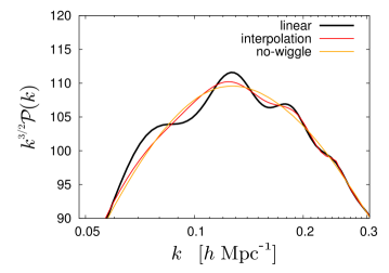
with a redshift-dependent smoothing scale (at ) calibrated by simulations [3]. For the no-wiggle portion of the spectrum, which taken by itself encapsulates the shape information in the data, two approaches have been used in the recent literature: a semi-analytic fitting formula, originally introduced in Ref. [29], and a cubic-spline interpolation of the linear power-spectrum given some fixed nodes.
While fine for standard CDM cosmology, the semi-analytic formula introduced in Ref. [29] per se does not describe cosmological models extended with massive neutrinos, a non-trivial equation of state for the dark energy, or non-standard relativistic degrees of freedom, to name a few. Extensions to the fitting formula of Ref. [29] to include a non-zero and have been investigated in Ref. [30] and [31] respectively. The second approach, the cubic-spline interpolation method of Ref. [3], bypasses completely the use of fitting formulae. Instead, it removes the BAO by singling out a reference set of oscillation nodes (corresponding to the WMAP5 best-fit vanilla model), which are then interpolated using a cubic spline. This method is correct as long as the chosen interpolation points coincide with the actual nodes of the BAO for a given cosmological model. However, in any model that tampers with the sound horizon relative to the reference case, e.g., by allowing to vary, the interpolation nodes and the actual nodes of the BAO can shift out of phase, thereby resulting in an insufficient removal of the baryon wiggles. We demonstrate an extreme example in Fig. 4.
Clearly, to ensure the nonlinear mode coupling is properly modelled in extended cosmological models, a more reliable way of constructing a smooth no-wiggle spectrum is needed. In this work, we have explored three different alternative ways to produce a no-wiggle spectrum: (i) a method based on a discrete spectral analysis of the power spectrum in log-space, (ii) a fourth order polynomial fit in , and (iii) a semi-analytic fitting formula with , and as free parameters built on the works of Refs. [29, 30, 31]. These are described in detail in the following subsections. The spectral method (i) is arguably by far the most elegant and generally applicable of the three alternative methods proposed here; all parameter estimation results presented in this work have been obtained using this approach.
A.1 Discrete spectral analysis
This approach is similar to considering the correlation function
| (2) |
in which the oscillations in appear as a bump [14]. Numerically, it is by far easier to identify a bump in an otherwise smooth function than it is to, e.g., find the zeros of the BAO in the power spectrum. Once the BAO bump has been identified and removed, the “de-bumped” correlation function can then be inverse Fourier-transformed to obtain a no-wiggle spectrum.
In practice, it turns out to be more efficient to use a discrete Fourier transform (more precisely, a fast sine transform [32]) instead of evaluating the integral (2). We have implemented the following algorithm to construct the no-wiggle spectrum:
-
1.
Sample in points, equidistant in .
-
2.
Do a fast sine transform of the array constructed in 1.
-
3.
Interpolate the odd and even entries of the resulting array using a cubic spline [32].
-
4.
Identify the baryonic bumps by determining where the second derivatives of the splines starts becoming large.
-
5.
Cut out the points corresponding to the baryonic bumps and fill in the gap by cubic spline interpolation.
-
6.
Do a reverse fast sine transform to recover .
For the models considered in this paper the effect on parameter estimates is relatively small, but nevertheless noticeable. Compared to results obtained with the spectral smoothing method, the fixed-node interpolation smoothing of Ref. [3] overestimates the uncertainty on and by roughly , and the error on by about in the vanilla+++ model. There is, however, no significant bias on the estimates of parameter means.
A.2 Fourth order polynomial fit
The polynomial fit method consists of replacing the logarithm of the power spectrum by a fourth-order polynomial in within the range , where is the turn-over scale of the spectrum (found automatically for each model), and is a scale fixed by the user (here, we take ). The idea is that to model the BAO wiggles with a simple polynomial would require that the polynomial contains as many maxima and minima as there are peaks and troughs in the wiggles. Thus if we keep the fitting polynomial at a sufficiently low order the wiggles will be automatically excluded from the fit.
A fourth order polynomial in principle has five free parameters, but since we impose continuity in and together with a zero derivative in , we only need to adjust two free parameters for each model. This is done using a simple least-square fit. We find in several independent runs that this method gives the same parameter estimates as the spectral method up to very high accuracy.
A.3 Semi-analytic fitting formula
The original fitting formula of Ref. [29] was extended in Ref. [30] to allow for a non-zero , and optimised for the case of one massive and two massless neutrinos, with held fixed at three. The relative error is estimated at the % level. Reference [31] further extended the work of Ref. [30] by including as a free parameter. This extension again assumed , but was optimised instead for and . In the present work, we perform yet another extension by relaxing the assumption of , so that and are two completely independent free parameters. Our code is built on that of Ref. [31].
In the following description of our modifications, however, we make frequent reference to [30] since the equations are better documented there.
-
1.
Equation (1) of [30] gives the redshift of matter-radiation equality as
(3) We modify this expression to
(4) where
(5) -
2.
Equation (5) of [30] introduces a normalised wavenumber ,
(6) where
(7) Here, we replace the expression for with
(8) - 3.
- 4.
For models with , and , the fitting formula is accurate to % at
Appendix B BAO data in extended models
Percival et al. [2] give the BAO likelihood in the form of a joint constraint on the parameters and , defined by
| (13) |
where
| (14) |
with the angular diameter distance , the Hubble parameter , and
| (15) |
is the comoving sound horizon. Here, the sound speed is given by
| (16) |
where is the ratio of baryon to photon momentum density.
The sound horizon (Eq.(15)) should in principle be evaluated at the baryon drag epoch , which is defined as the redshift at which the drag optical depth equals one, i.e.,
| (17) | |||||
with today’s baryon and photon densities , , the Thomson cross-section and the fraction of free electrons . However, Percival et al. use the approximation obtained from a (somewhat outdated) fitting formula (Eq.(4) of Eisenstein & Hu [29]) instead. The fact that the results of the fitting formula are inaccurate by several per cent is not a problem per se, since is only used as a proxy in the data processing, as discussed in Section 4 of Ref. [2], and as long as one considers simple cosmologies, the dependence of on cosmological parameters is likely to be adequately represented.
One should keep in mind though that the Eisenstein & Hu fitting formula was derived under certain assumptions (e.g., is fixed to a value of 3). So for instance in models in which is a free parameter, the fitting formula will no longer faithfully capture the proper parameter dependencies. In these cases, an unreflected use of the default BAO likelihood code as implemented in the October 2009 version of CosmoMC will lead to biased results. However, this deficiency can be remedied by simple rescaling. Instead of using as defined in Equation (13) as input for the BAO likelihood code, we perform the substitution
| (18) |
where is evaluated for the fiducial cosmology of Ref. [2], and computed numerically by solving Equation (17). This quantity has the correct dependence on all cosmological parameters and will yield unbiased parameter and error estimates.
References
- [1] E. Komatsu et al., arXiv:1001.4538 [astro-ph.CO].
- [2] W. J. Percival et al., Mon. Not. Roy. Astron. Soc. 401 (2010) 2148 [arXiv:0907.1660 [astro-ph.CO]].
- [3] B. A. Reid et al., arXiv:0907.1659 [astro-ph.CO].
- [4] R. Biswas and B. D. Wandelt, arXiv:0903.2532 [astro-ph.CO].
- [5] B. A. Reid, L. Verde, R. Jimenez and O. Mena, JCAP 1001 (2010) 003 [arXiv:0910.0008 [astro-ph.CO]].
- [6] D. Larson et al., arXiv:1001.4635 [astro-ph.CO].
- [7] C. L. Reichardt et al., Astrophys. J. 694 (2009) 1200 [arXiv:0801.1491 [astro-ph]].
- [8] H. C. Chiang et al., arXiv:0906.1181 [astro-ph.CO].
- [9] M. L. Brown et al. [QUaD collaboration], Astrophys. J. 705 (2009) 978 [arXiv:0906.1003 [astro-ph.CO]].
- [10] A. G. Riess et al., Astrophys. J. 699 (2009) 539 [arXiv:0905.0695 [astro-ph.CO]].
- [11] F. Finelli, J. Hamann, S. M. Leach and J. Lesgourgues, arXiv:0912.0522 [astro-ph.CO].
- [12] A. Lewis and S. Bridle, Phys. Rev. D 66 (2002) 103511 [arXiv:astro-ph/0205436].
- [13] A. Gelman and D. B. Rubin, Statistical Science 7 (1992) 457.
- [14] D. J. Eisenstein et al. [SDSS Collaboration], Astrophys. J. 633 (2005) 560 [arXiv:astro-ph/0501171].
- [15] J. Hamann, S. Hannestad, G. G. Raffelt and Y. Y. Y. Wong, JCAP 0708 (2007) 021 [arXiv:0705.0440 [astro-ph]].
- [16] [Planck Collaboration], arXiv:astro-ph/0604069.
- [17] L. Perotto, J. Lesgourgues, S. Hannestad, H. Tu and Y. Y. Y. Wong, JCAP 0610 (2006) 013 [arXiv:astro-ph/0606227].
- [18] J. Lesgourgues and S. Pastor, Phys. Rept. 429 (2006) 307 [arXiv:astro-ph/0603494].
- [19] E. Komatsu et al. [WMAP Collaboration], Astrophys. J. Suppl. 180 (2009) 330 [arXiv:0803.0547 [astro-ph]].
- [20] S. A. Thomas, F. B. Abdalla and O. Lahav, arXiv:0911.5291 [astro-ph.CO].
- [21] Y. S. Song and L. Knox, Phys. Rev. D 70 (2004) 063510 [arXiv:astro-ph/0312175].
- [22] J. Lesgourgues, S. Pastor and L. Perotto, Phys. Rev. D 70, 045016 (2004) [arXiv:hep-ph/0403296].
- [23] S. Wang, Z. Haiman, W. Hu, J. Khoury and M. May, Phys. Rev. Lett. 95, 011302 (2005) [arXiv:astro-ph/0505390].
- [24] S. Hannestad and Y. Y. Y. Wong, JCAP 0707, 004 (2007) [arXiv:astro-ph/0703031].
- [25] A. Vikhlinin et al., Astrophys. J. 692, 1060 (2009) [arXiv:0812.2720 [astro-ph]].
- [26] J. R. Pritchard and E. Pierpaoli, Nucl. Phys. Proc. Suppl. 188, 31 (2009).
- [27] A. Rassat et al., arXiv:0810.0003 [astro-ph].
- [28] D. J. Eisenstein, H. J. Seo and M. J. White, Astrophys. J. 664 (2007) 660 [arXiv:astro-ph/0604361].
- [29] D. J. Eisenstein and W. Hu, Astrophys. J. 496 (1998) 605 [arXiv:astro-ph/9709112].
- [30] D. J. Eisenstein and W. Hu, Astrophys. J. 511 (1997) 5 [arXiv:astro-ph/9710252].
- [31] A. Kiakotou, Ø. Elgarøy and O. Lahav, Phys. Rev. D 77 (2008) 063005 [arXiv:0709.0253 [astro-ph]].
- [32] W. H. Press, S. A. Teukolsky, W. T. Vetterling and B. P. Flannery, “Numerical Recipes in Fortran,” Cambridge University Press (1992).