Dissimilarity maps on trees and and the representation theory of $SL_{m}(\mathbb{C})$

Abstract.

We prove that $m$-dissimilarity vectors of weighted trees are points on the tropical Grassmannian, as conjecture by Cools in response to a question of Sturmfels and Pachter. We accomplish this by relating $m$-dissimilarity vectors to the representation theory of $SL_{m}(\mathbb{C}).$

1. Introduction

We will explore tropical properties of weighted, or metric trees $\mathcal{T},$ using the representation theory of the special linear group $SL_{m}(\mathbb{C}).$ We direct the reader to the book by Fulton and Harris [FH] and the book by Dolgachev [D] for an introduction to the representation theory of connected complex reductive groups over $\mathbb{C}$. Recall that we can choose a Borel subgroup $B$, and a maximal torus $T$ with $T\subset B\subset G,$ and associate to this data a monoid of weights $C_{G}\subset X(T)$ in the characters of $T,$ which classify irreducible representations of $G$ up to isomorphism. This cone comes with an involution defined by the duality operation on representations $\lambda\to\lambda^{*}.$ The direct sum of all such representations forms a commutative algebra

(1) $$R(G)=\bigoplus_{\lambda\in C_{G}}V(\lambda^{*})$$

which is the coordinate ring of the quotient of $G$ by the unipotent radical of a chosen Borel subgroup, $R(G)=\mathbb{C}[G/U].$ For $SL_{m}(\mathbb{C})$, this can be taken to be the subgroup of unipotent upper-triangular matrices. Choosing a Borel subgroup also fixes a set of positive roots $R_{+}\subset X(T),$ for $G,$ which define a partial ordering on the weights, we say that $\lambda\geq\lambda^{\prime}$ if $\lambda-\lambda^{\prime}$ is a member of $\mathbb{N}R_{+}.$ For $SL_{m}(\mathbb{C}),$ the cone $C_{SL_{m}(\mathbb{C})}$ is generated over $\mathbb{Z}_{+}$ by $m-1$ fundamental weights, $\omega_{1},\ldots,\omega_{m-1}.$ The weight $\omega_{i}$ is the so-called highest weight of the representation $\bigwedge^{i}(\mathbb{C}^{m}).$ The main result of this paper expresses the $m$-dissimilarity vector of an arbitrary tree in terms of the fundamental weights of $SL_{m}(\mathbb{C})$. In what follows $A_{+}$ denotes the non-negative members of $A=\mathbb{Z}$ or $\mathbb{R}.$

1.1. Dissimilarity maps and the Grassmannian

Let $\mathcal{T}$ be a trivalent tree with $n$ ordered leaves, and let $\ell:Edge(\mathcal{T})\to\mathbb{R}_{+}$ be a function which assigns a weight (or length) to each edge of $\mathcal{T}.$ The weight function $\ell$ defines a metric on the leaves $L(\mathcal{T})$ of $\mathcal{T},$ where the distance $d_{ij}$ between the leaves $i$ and $j$ is the sum of the weights on the edges of the unique path $\gamma(i,j)$ connecting $i$ to $j$ in $\mathcal{T}.$ We intentionally confuse the path $\gamma_{ij}$ with the set of edges it traverses.

(2) $$d_{ij}(\mathcal{T},\ell)=\sum_{e\in\gamma(i,j)}\ell(e)\\$$

Obviously $d_{ij}=d_{ji}$ and $d_{ii}=0.$ We call the vector $D_{2,n}(\mathcal{T},\ell)=\{d_{ij}(\mathcal{T},\ell)\}_{i<j}\in\mathbb{R}^{\binom{n}{2}}$ the $2$-dissimilarity vector of $(\mathcal{T},\ell).$ We may generalize this construction by introducing the convex hull of $m$ leaves $i_{1}\ldots i_{m}\in L(\mathcal{T})$ as the set of all edges which appear in paths connecting some $i_{j}$ to some $i_{k}.$

(3) $$\gamma(i_{1}\ldots i_{m})=\bigcup\gamma(i_{j}i_{k})\\$$

The $m$-dissimilarity vector $D_{m,n}(\mathcal{T},\ell)=\{d_{i_{1}\ldots i_{m}}(\mathcal{T},\ell)\}_{i_{1}<\ldots<i_{m}}\in\mathbb{R}^{\binom{n}{m}}$ is then defined as expected.

(4) $$d_{i_{1}\ldots i_{m}}(\mathcal{T},\ell)=\sum_{e\in\gamma(i_{1}\ldots i_{m})}\ell(e)\\$$

Figure 1. The convex hull of three leaves

The set of $2$-dissimilarity vectors of weighted trees $T_{2,n}\subset\mathbb{R}^{\binom{n}{2}}$ is well understood. A weighted tree can be recovered from its $2$-dissimilarity vector, and the set of all $2$-dissimilarity vectors is characterized by the following theorem from tropical geometry, see [SpSt], [C].

Theorem 1.1.

The set of $2$-dissimilarity vectors coincides with the tropical Grassmanian.

$$T_{2,n}=Trop(Gr_{2}(\mathbb{C}^{n}))\subset\mathbb{R}^{\binom{n}{2}}$$

The Gröbner fan of the Plücker algebra $\mathbb{C}[X_{i_{1},\ldots,i_{m}}]/I_{m,n}$ has support $\mathbb{R}^{\binom{n}{m}},$ so each vector $w$ in this space gives a Gröbner degeneration of the ideal $I_{m,n}$ to the ideal of initial forms $in_{w}(I_{m,n})$. The set of vectors $w$ which for which $in_{w}(I_{m,n})$ is monomial free is called the tropical Grassmannian $Trop(Gr_{m}(\mathbb{C}^{n})).$ The above theorem implies that for a vector $w\in\mathbb{R}^{\binom{n}{2}}$ to be a $2$-dissimilarity vector, it must weight Plücker variables $z_{ij}$ in such a way that at least two monomials in each Plücker relation

(5) $$z_{ij}z_{k\ell}-z_{ik}z_{j\ell}+z_{i\ell}z_{jk}\\$$

have the same weight. For a point $\vec{w}=\{w_{ij}\}$ to satisfy this requirement, the maximum of $\{w_{ij}+w_{k\ell},w_{ik}+w_{j\ell},w_{i\ell}+w_{jk}\}$ must be obtained at least twice. If this is the case, then we may find a tree $(\mathcal{T},\ell)$ such that $d_{i,j}(\mathcal{T},\ell)=w_{ij}.$ Since $2$-dissimilarity vectors characterize their respective weighted trees, we should expect that some operation on the $2$-dissimilarity vector of a weighted tree $(\mathcal{T},\ell)$, probably tropical in nature, will yield the $m$-dissimiliarity vector, and indeed this is the case, see [BC] for the following theorem.

Theorem 1.2.

Let $\mathcal{C}_{m}$ be the set of length $m$ cycles in the set of permutations on $m$ letters. Then we have the following formula.

(6) $$d_{i_{1}\ldots i_{m}}(\mathcal{T},\ell)=\frac{1}{2}min_{\alpha\in C_{m}}\{d_{i_{1}i_{\alpha(1)}}(\mathcal{T},\ell)+\ldots+d_{i_{\alpha^{m-1}(1)}i_{\alpha^{m}(1)}}(\mathcal{T},\ell)\}\\$$

This defines an onto map $\phi^{(m)}:T_{2,n}\to T_{m,n}.$

Given that $T_{m,n}$ and the tropical Grassmannian $Trop(Gr_{m}(\mathbb{C}^{n}))$ live in the same space, and coincide for $m=2,$ one would hope that these two sets always have a close relationship. Sturmfels and Pachter asked if the set of $m$-dissimilarity vectors was always contained in the tropical Grassmannian $Trop(Gr_{m}(\mathbb{C}^{n},)$ [PSt]. Cools recently proved this for small $m,$ [C] and conjectured that the result holds for all $m,$ the result was proved in general by Giraldo, [G].

Theorem 1.3 (Cools, Giraldo).

(7) $$\phi^{(m)}(T_{2,n})=T_{m,n}\subset Trop(Gr_{m}(\mathbb{C}^{n}))\\$$

This means that the entries of $D_{m,n}(\mathcal{T},\ell)$ always satisfy the tropical Plücker equations, and the weighting defined by this vector defines a monomial free initial ideal $in_{D_{m,n}(\mathcal{T},\ell)}(I_{m,n}).$ The purpose of this note is to prove this theorem using tropical properties of the Plücker algebra deduced from the related representation theory of $SL_{m}(\mathbb{C})$.

1.2. Invariants in tensor products of representations.

The Plücker algebra $\mathbb{C}[X_{i_{1},\ldots,i_{m}}]/I_{m,n}$ is a natural object in the representation theory of $SL_{m}(\mathbb{C}),$ it appears as the subring of invariants of the diagonal action of $SL_{m}(\mathbb{C})$ on $M_{m\times n}(\mathbb{C}),$ this is the First Fundamental Theorem of Invariant Theory.

(8) $$\mathbb{C}[X_{i_{1},\ldots,i_{m}}]/I_{m,n}\cong\mathbb{C}[M_{m\times n}(\mathbb{C})]^{SL_{m}(\mathbb{C})}\\$$

The Plücker algebra is exactly the subring generated by the Plücker coordinates, $Z_{i_{1}\ldots i_{m}}$. Let $A\in M_{m\times n}(\mathbb{C}),$ $A=[C_{1}\ldots C_{n}],$ with $C_{i}\in\mathbb{C}^{m},$ then the value of the Plücker coordinates at $A$ is defined by the following.

(9) $$Z_{i_{1}\ldots i_{m}}(A)=det[C_{i_{1}}\ldots C_{i_{m}}]\\$$

We may rewrite this algebra in terms of the category of finite dimensional representations of $SL_{m}(\mathbb{C})$ as follows.

(10) $$\mathbb{C}[M_{m\times n}(\mathbb{C})]^{SL_{m}(\mathbb{C})}=\bigoplus_{\vec{r}\in\mathbb{Z}_{+}^{n}}[V(r_{1}\omega_{1}^{*})\otimes\ldots\otimes V(r_{n}\omega_{1}^{*})]^{SL_{m}(\mathbb{C})}\\$$

Here $\omega_{1}$ is the highest weight of $\mathbb{C}^{m}$ as a representation of $SL_{m}(\mathbb{C})$ and $\omega_{1}^{*}=\omega_{m-1}$. With respect to this direct-sum decomposition, the Plücker coordinate $Z_{i_{1}\ldots i_{m}}$ is a generator of the summand with $V(\omega_{1}^{*})$ in the $r_{i_{j}}-$th place for all $i_{j}\in\{i_{1},\ldots,i_{m}\},$ and the trivial representation everywhere else. Multiplication in $\mathbb{C}[M_{m,n}(\mathbb{C})]$ has a nice description in terms of this direct sum decomposition as well, it is induced by the Cartan multiplication maps in each component, where the tensor product is projected onto its highest weight summand.

(11) $$V(r_{1}\omega_{1}^{*})\otimes V(r_{2}\omega_{1}^{*})\to V((r_{1}+r_{2})\omega_{1}^{*})\\$$

We may rewrite each summand in terms of homomorphisms from the category of $SL_{m}(\mathbb{C})$ representations.

(12) $$[V(r_{1}\omega_{1}^{*})\otimes\ldots\otimes V(r_{n}\omega_{1}^{*})]^{SL_{m}(\mathbb{C})}=Hom_{SL_{m}(\mathbb{C})}(\mathbb{C},V(r_{1}\omega_{1}^{*})\otimes\ldots\otimes V(r_{n}\omega_{1}^{*}))\\$$

In this way, the Plücker algebra encodes the branching problem of finding copies of the trivial representation of $SL_{m}(\mathbb{C})$ in an irreducible representation of $SL_{m}(\mathbb{C})^{n}.$ For this reason, we will refer to the Plücker algebra as a branching algebra. In general, a branching algebra encodes the branching rules of irreducible representations for some map of reductive groups. In this case the map is the diagonal map $\Delta_{n}:SL_{m}(\mathbb{C})\to SL_{m}(\mathbb{C})^{n}.$ Filtrations and associated graded algebras of branching algebras like this one were studied by the author in [M], in particular for diagonal embeddings as above, the author described a way to produce filtrations of the branching algebra associated to labelled, rooted trees. We will review the details of this construction in the next section, but for now we will describe the features that we need. Let $C_{SL_{m}(\mathbb{C})}$ be the cone of dominant weights with respect to the standard ordering of weight vectors in the weight lattice for $SL_{m}(\mathbb{C}).$ Let $\hat{\mathcal{T}}$ be a rooted tree with $n$ leaves, we consider the orientation induced on the edges of $\hat{\mathcal{T}}$ by orienting every edge in the unique path from the root to a leaf in such a way to make the root the unique source.

Proposition 1.4.

Let $\hat{\mathcal{T}}$ be a rooted tree with $n$ leaves. There is a direct-sum decomposition,

(13) $$[V(r_{1}\omega_{1})\otimes\ldots\otimes V(r_{n}\omega_{1})]^{SL_{m}(\mathbb{C})}=\bigoplus\mathcal{W}(\hat{\mathcal{T}},\lambda)\\$$

over all $\lambda:Edge(\hat{\mathcal{T}})\to C_{SL_{m}(\mathbb{C})},$ such that the root edge is weighted $0,$ the edge incident to the $i$’th leaf is weighted $r_{i}\omega_{1}^{*},$ and for each internal vertex, the representation associated to the label on the sink appears in the direct sum decomposition of the tensor product of the representations associated to the labels on the sources. The summand $\mathcal{W}(\hat{\mathcal{T}},\lambda)$ is the vector space of all possible assignments of intertwiners to the internal vertices which realize the weight on a source at a vertex as a summand of the tensor product of the weights on sinks.

In figure 2 we an example of such an object with $SL_{m}(\mathbb{C})$ representations given by Young tableaux. Recall that $\omega_{1}^{*}=\omega_{m-1}.$

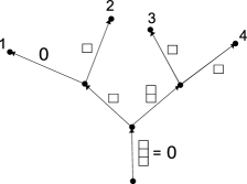
Figure 2. A tree weighted with representations

Proposition 1.4 is a formal consequence of properties of semisimple categories with monoidal products. The tree $\hat{\mathcal{T}}$ can be considered as a recipe for inserting parentheses into the tensor product $V(r_{1}\omega_{1}^{*})\otimes\ldots\otimes V(r_{n}\omega_{1}^{*}),$ and gives a way to recursively expand the expression into a direct sum. We can then take the same tree $\hat{\mathcal{T}}$ and assign to its edges $e\in Edge(\mathcal{T})$ functionals $h_{e}:C_{SL_{m}(\mathbb{C})}\subset X(T_{SL_{m}(\mathbb{C})})\to\mathbb{R}_{+},$ taking care that $h_{e}$ is positive on all positive roots. We apply this functional $(\hat{\mathcal{T}},\hat{h})$ to each summand, where an element in $\mathcal{W}(\hat{\mathcal{T}},\lambda)$ is given the weight $\sum_{e\in Edge(\hat{\mathcal{T}})}h_{e}(\lambda(e)).$ This weights each Plücker coordinate $Z_{i_{1}\ldots i_{m}}$ with a number dependent on $\hat{h}$ and the tree $\hat{\mathcal{T}},$ and so gives a point in $\mathbb{R}^{\binom{n}{m}}.$ After reviewing the construction of this filtration and understanding it with respect to the multiplication operation in the Plücker algebra, we will be able to conclude the following.

Theorem 1.5.

Each $(\hat{\mathcal{T}},\hat{h})$ defines a point in $Trop(Gr_{m}(\mathbb{C}^{n}))\subset\mathbb{R}^{\binom{n}{m}}$

This will follow from general arguments on filtrations of branching algebras obtained from the associated representation theory, in particular we will give a general way to produce points on the tropical varieties of ideals defining these algebras. The functionals $(\hat{\mathcal{T}},\hat{h})$ have a good amount of flexibility, enough to show the following theorem.

Theorem 1.6.

There exists for any weighted tree $(\mathcal{T},\ell)$ a tree functional $(\hat{\mathcal{T}},\hat{h})$ such that $d_{i_{1}\ldots i_{m}}(\mathcal{T},\ell)=(\hat{\mathcal{T}},\hat{h})(Z_{i_{1}\ldots i_{m}})$ for all $m$ tuples $\{i_{1},\ldots,i_{m}\}.$ In particular, $m$-dissimilarity vectors are points on the tropical Grassmannian.

1.3. Acknowledgements

We thank the reviewer for several useful suggestions, including the example 2.3.

2. Filtrations of branching algebras

In this section we will review the construction of filtrations of branching algebras introduced in [M]. The basic object we will be working with is the algebra $R(G)=\mathbb{C}[G]^{U_{G}}=\bigoplus_{\lambda\in C_{G}}V(\lambda^{*}),$ where $G$ is a connected reductive group over $\mathbb{C}$, $U_{G}\subset G$ is a maximal unipotent subgroup, $\lambda$ are dominant weights, $V(\lambda)$ is the irreducible representation with highest weight $\lambda,$ and $C_{G}$ is the monoid of dominant weights. We choose highest weight vectors for each irreducible representation $v_{\lambda}\in V(\lambda).$ Multiplication in $R(G)$ is induced by Cartan multiplication, see [AB] for an introduction to the algebra $R(G)$.

$$\begin{CD}V(\alpha^{*})\otimes V(\beta^{*})@>{C_{*}}>{}>V(\alpha^{*}+\beta^{*})\\ \end{CD}$$

Identify $V(\lambda^{*})$ with the dual $V(\lambda)^{*}$ in the unique way that makes $ev(v_{\lambda},\hat{v}_{\lambda^{*}})=1$ where $ev:V(\lambda)\otimes V(\lambda)^{*}\to\mathbb{C}$ sends $v\otimes f$ to $f(v),$ and $\hat{v}_{\lambda^{*}}$ is the lowest weight vector of $V(\lambda^{*}).$ Under this identification, Cartan multiplication is the dual of the map which sends $v_{\alpha+\beta}$ to $v_{\alpha}\otimes v_{\beta}$.

$$\begin{CD}V(\alpha+\beta)@>{C^{*}}>{}>V(\alpha)\otimes V(\beta)\\ \end{CD}$$

Let $\phi:H\to G$ be a map of connected reductive groups over $\mathbb{C},$ we define the branching algebra $\mathfrak{A}(\phi)$ of $\phi$ as follows.

(14) $$\mathfrak{A}(\phi)=[R(H)\otimes R(G)]^{H}=\bigoplus_{(\alpha,\beta)\in C_{H}\times C_{G}}[V(\alpha^{*})\otimes W(\beta^{*})]^{H}\\$$

Here $H$ acts on $R(G)$ through $\phi,$ and $\phi$ maps $U_{H}$ to $U_{G}.$ Branching algebras are so-named because the dimension of their multigraded components give the branching multiplicities for irreducible representations of $G$ as representations of $H.$ We will now rewrite the multiplication operation in $\mathfrak{A}(\phi)$ with respect to the following identity.

(15) $$[V(\alpha^{*})\otimes W(\beta^{*})]^{H}=Hom_{H}(\mathbb{C},V(\alpha^{*})\otimes W(\beta^{*}))\cong Hom_{H}(V(\alpha),W(\beta^{*}))\\$$

The isomorphism on the right is given by the following construction, for $f\in Hom_{H}(\mathbb{C},V(\alpha^{*})\otimes W(\beta^{*}))$.

$$\begin{CD}V(\alpha)=V(\alpha)\otimes\mathbb{C}@>{id\otimes f}>{}>V(\alpha)\otimes V(\alpha^{*})\otimes W(\beta^{*})@>{ev\otimes id}>{}>W(\beta^{*})\\ \end{CD}$$

Let $\hat{f}=(ev\otimes id)\circ(id\otimes f)$ denote the transformed map. Under this isomorphism, the multiplication map

$$\begin{CD}\mathbb{C}\otimes\mathbb{C}@>{f\otimes g}>{}>[V(\alpha_{1}^{*})\otimes W(\beta_{1}^{*})]\otimes[V(\alpha_{2}^{*})\otimes W(\beta_{2}^{*})]@>{C_{*}\otimes C_{*}}>{}>V(\alpha_{1}^{*}+\alpha_{2}^{*})\otimes W(\beta_{1}^{*}+\beta_{2}^{*})\\ \end{CD}$$

becomes

$$\begin{CD}V(\alpha_{1}+\alpha_{2})@>{C^{*}}>{}>V(\alpha_{1})\otimes V(\alpha_{2})@>{\hat{f}\otimes\hat{g}}>{}>W(\beta_{1}^{*})\otimes W(\beta_{2}^{*})@>{C_{*}}>{}>W(\beta_{1}^{*}+\beta_{2}^{*})\\ \end{CD}$$

this is a straightforward calculation. Now we consider a factorization of $\phi$ in the category of connected reductive groups over $\mathbb{C}.$

$$\begin{CD}H@>{\psi}>{}>K@>{\pi}>{}>G\\ \end{CD}$$

We formally get a direct sum decomposition of each multigraded component of the branching algebra $\mathfrak{A}(\phi).$

(16) $$Hom_{H}(V(\alpha),W(\beta^{*}))=\bigoplus_{\eta\in C_{K}}Hom_{H}(V(\alpha),Y(\eta^{*}))\otimes Hom_{K}(Y(\eta^{*}),W(\beta^{*}))\\$$

This introduces a host of combinatorial representation theory data into the algebra $\mathfrak{A}(\phi).$ We will see how to multiply two elements, we start by taking the tensor product.

$$\begin{CD}V(\alpha_{1})\otimes V(\alpha_{2})@>{f_{1}\otimes f_{2}}>{}>Y(\eta_{1}^{*})\otimes Y(\eta_{2}^{*})@>{g_{1}\otimes g_{2}}>{}>W(\beta_{1}^{*})\otimes W(\beta_{2}^{*})\\ \end{CD}$$

The middle representation decomposes as a direct sum of $K$ representations,

(17) $$Y(\eta_{1}^{*})\otimes Y(\eta_{2}^{*})=\bigoplus_{\eta\in C_{K}}Hom_{K}(Y(\eta^{*}),Y(\eta_{1}^{*})\otimes Y(\eta_{2}^{*}))\otimes Y(\eta^{*})\\$$

this allows us to represent $f_{1}\otimes f_{2}$ and $g_{1}\otimes g_{2}$ as sums of maps. Let $\pi_{\eta}:Y(\eta_{1}^{*})\otimes Y(\eta_{2}^{*})\to Hom_{K}(Y(\eta^{*}),Y(\eta_{1}^{*})\otimes Y(\eta_{2}^{*}))\otimes Y(\eta^{*})$ and $\pi^{\eta}:Hom_{K}(Y(\eta^{*}),Y(\eta_{1}^{*})\otimes Y(\eta_{2}^{*}))\otimes Y(\eta^{*})\to Y(\eta_{1}^{*})\otimes Y(\eta_{2}^{*})$ be projections and injections that define the direct sum decomposition with $\pi_{\eta_{1}+\eta_{2}}=C_{*}$ and $\pi^{\eta_{1}+\eta_{2}}=C^{*}.$ Then we have

(18) $$f_{1}\otimes f_{2}=\sum\pi_{\eta}\circ(f_{1}\otimes f_{2}),\\$$

(19) $$g_{1}\otimes g_{2}=\sum(g_{1}\otimes g_{2})\circ\pi^{\eta}\\$$

Decomposing the diagram along these sums gives an expansion of the product into components from the direct sum decomposition of $Hom_{H}(V(\alpha_{1}+\alpha_{2}),W(\beta_{1}+\beta_{2}))$, and there is a natural leading term given by the sum of the weights,

$$\begin{CD}V(\alpha_{1}+\alpha_{2})@>{C_{*}\circ(f_{1}\otimes f_{2})\circ C^{*}}>{}>Y(\eta_{1}^{*}+\eta_{2}^{*})@>{C_{*}\circ(g_{1}\otimes g_{2})\circ C^{*}}>{}>W(\beta_{1}^{*}+\beta_{2}^{*}).\\ \end{CD}$$

A general term,

$$\begin{CD}V(\alpha_{1}+\alpha_{2})@>{\pi_{\eta}\circ(f_{1}\otimes f_{2})\circ C^{*}}>{}>Y(\eta^{*})@>{C_{*}\circ(g_{1}\otimes g_{2})\circ\pi^{\eta}}>{}>W(\beta_{1}^{*}+\beta_{2}^{*}).\\ \end{CD}$$

is a member of the $(\alpha_{1}+\alpha_{2},\eta,\beta_{1}+\beta_{2})$ summand. The leading term never vanishes, because the defining maps $C_{*}\circ(f_{1}\otimes f_{2})\circ C^{*}$ and $C_{*}\circ(g_{1}\otimes g_{2})\circ C^{*}$ are the same as the multiplication operation in $\mathfrak{A}(\psi)$ and $\mathfrak{A}(\pi)$ respectively. These algebras are domains because $R(G)$ is always a domain. Notice that this analysis depends only on multigraded summands of $\mathfrak{A}(\phi),$ so the same term decomposition exists for any subalgebra which preserves the multigrading. We summarize the previous discussion.

Proposition 2.1.

For any factorization of a map of connected, reductive groups over $\mathbb{C},$

$$\begin{CD}H@>{\psi}>{}>K@>{\pi}>{}>G\end{CD}$$

there is a direct sum decomposition of $\mathfrak{A}(\phi)$ into summands $\mathcal{W}(\alpha,\eta,\beta),$ with $\alpha\in C_{H},$ $\eta\in C_{K}$ and $\beta\in C_{G}$ dominant weights. This defines a multifiltration of the branching algebra $\mathfrak{A}(\pi\circ\psi).$ The product of two elements

$$\begin{CD}V(\alpha_{1})@>{f_{1}}>{}>Y(\eta_{1})@>{g_{1}}>{}>W(\beta_{1})\\ V(\alpha_{2})@>{f_{2}}>{}>Y(\eta_{2})@>{g_{2}}>{}>W(\beta_{2})\\ \end{CD}$$

has leading term

$$\begin{CD}V(\alpha_{1}+\alpha_{2})@>{C_{*}\circ f_{1}\otimes f_{2}\circ C^{*}}>{}>Y(\eta_{1}+\eta_{2})@>{C_{*}\circ g_{1}\otimes g_{2}\circ C^{*}}>{}>W(\beta_{1}+\beta_{2}).\\ \end{CD}$$

all lower terms involve $\eta\in C_{K}$ which are less than $\eta_{1}+\eta_{2}$ as dominant weights.

We can perform this same construction on a factorization of any length

$$\begin{CD}H@>{\psi}>{}>K_{1}@>{\pi_{1}}>{}>\ldots @>{\pi_{k-1}}>{}>K_{k}@>{\pi}>{}>G\\ \end{CD}$$

without altering the details, and proposition 2.1 holds for the resulting multifiltration. We may use this extra combinatorial data to describe filtrations of $\mathfrak{A}(\phi).$ To each new summand $\mathcal{W}(\alpha,\vec{\lambda},\beta)$ in the filtration, we attach a number as follows, pick functionals

(20) $$h_{0}:X(T_{H})\to\mathbb{R}_{+},\\ h_{1}:X(T_{K_{1}})\to\mathbb{R}_{+},\\ \dots,\\ h_{k}:X(T_{K_{k}})\to\mathbb{R}_{+},\\ h_{k+1}:X(T_{G})\to\mathbb{R}_{+},\\$$

such that $h_{i}$ has non-negative value on all positive roots of $K_{i}$. Now apply these functionals to the weights defining the multifiltered summands, this defines a filtration.

$$\begin{CD}\vec{h}(V(\lambda_{0})@>{f_{1}}>{}>V(\lambda_{1})@>{f_{2}}>{}>\ldots @>{f_{k}}>{}>V(\lambda_{k}))=\sum h_{i}(\lambda_{i})\\ \end{CD}$$

By proposition 2.1, the value on a product of elements, computed by summing up the contributions from each element, is always equal to the value on its leading term for any linear functional $\vec{h}.$

Proposition 2.2.

Let $\Phi:\mathbb{C}[X]\to\mathfrak{A}(\phi)$ be a presentation of the branching algebra, and let $\phi=\psi_{1}\circ\ldots\psi_{k}$ be a factorization of $\phi.$ Suppose each $x\in X$ is mapped to an element of one of the summands $\mathcal{W}(\vec{\lambda})\subset\mathfrak{A}(\phi)$ defined by the factorization, and let $I\subset\mathbb{C}[X]$ be the defining ideal. Then any functional $\vec{h}$ defines a term weighting of $X$ which gives a monomial free initial ideal $in_{\vec{h}}(I)$.

Proof.

Pick any expression in the ideal $I$.

(21) $$F(X)=\sum c_{a}\vec{x}^{\vec{a}}\\$$

We consider the expansion of each monomial term into pure terms, $\Phi\circ(\vec{x}^{\vec{a}})=S_{0}^{a}+\ldots+S_{m}^{a},$ where $S_{0}^{a}$ has the same pure filtration level as the monomial, the existence of this term follows from proposition 2.1, which also implies that we must have $\vec{h}(S_{0})\geq\vec{h}(S_{i})$ for every term in this expansion. In general, for pure terms $X$ and $Y$, we say that $X\geq Y$ if for each component $\lambda_{i}(X)-\lambda_{i}(Y)$ is a positive root. Note that not all pure terms are comparable. By definition of the functional $\vec{h}$ if $X\leq Y$ then $\vec{h}(X)\leq\vec{h}(Y).$ Now suppose some monomial $\vec{x}^{\vec{a}}$ in the expression $F(X)$ has the highest filtration weight with respect to $\vec{h}.$ We must have $\Phi\circ F(X)=0,$ so $S_{0}^{\vec{a}}$ must be canceled by pure terms from the expansion of other monomials. This implies that some monomial $\vec{x}^{\vec{b}}$ must have a pure term $S_{j}^{\vec{b}}$ with the same multifiltration level as $S_{0}^{\vec{a}}.$ We must have that $S_{0}^{\vec{a}}\leq S_{0}^{\vec{b}}$ as pure terms, by assumption this implies that $\vec{x}^{\vec{b}}$ has the same filtration weight as $\vec{x}^{\vec{a}}$. ∎

This proposition implies that every $\vec{h}$ defines a point on the tropical variety of the defining ideal $I.$ It also implies that for any presentation $\Phi:\mathbb{C}[X]\to\mathfrak{A}(\phi),$ and any form in the defining ideal $F(X)\in I,$ the leading terms of at least two monomials agree, a result independent of a functional $\vec{h}.$ The functionals $\vec{h}$ fit into the broader theory of valuations on rings. Roughly these are functions $v$ on a ring which satisfy $v(ab)=v(a)+v(b),$ $v(a+b)\leq max\{v(a),v(b)\},$ and $v(0)$ is $0$ or $-\infty$ depending on the tropical algebra where $v$ takes its values. Generally speaking valuations define ”universal” tropical points, in that they define a point on the tropical variety of any presentation of a subring of the ring on which they are defined. We explore these objects in the note [M2], see also [P]. For each factorization of $\phi:H\to G$

(22) $$F=\{\psi_{1},\ldots,\psi_{k}\},\\$$

(23) $$\phi=\psi_{1}\circ\ldots\circ\psi_{k}\\$$

we obtain a cone of functionals $\vec{h}\in P_{F}$ defined by the conditions on the components of $\vec{h}.$ Note that the $h_{i}=0$ is always an option, indeed this essentially forgets the information in $i$-th component of the multifiltration. For each factorization $F=\{\psi_{1},\ldots,\psi_{k}\}$ and every $i,$ there is an operation

(24) $$O_{i}(F)=\{\psi_{1}\ldots,\psi_{i-1},\psi_{i+1}\circ\psi_{i},\psi_{i+2},\ldots,\psi_{k}\}\$$

Setting $h_{i}$ to $0$ gives a map of cones $P_{O_{i}(F)}\to P_{F}$ which defines $P_{O_{i}(F)}$ as a face of $P_{F}.$ This defines a connected complex of cones $\bigcup_{F\circ\phi}P_{F}$ over all factorizations of $\phi$ in the category of connected, reductive groups. The content of the proposition above is that there is a map from this complex into the tropical variety of any presentation of $\mathfrak{A}(\phi),$ the same holds for any subalgebra of $B\to\mathfrak{A}(\phi)$ which preserves the multigrading. In particular, this is true for the subalgebra of invariants, which will be important in the sequel.

(25) $$R(G)^{H}=[\mathbb{C}\otimes R(G)]^{H}\subset[R(H)\otimes R(G)]^{H}=\mathfrak{A}(\phi),\\$$

Example 2.3.

We can also look at branching deformations for the trivial subgroup of a reductive group $1\to G.$ This morphism is factored by any flag of subgroups of $G,$ for instance we can take $G=GL_{n}$ and look at the flag

(26) $$1\to GL_{1}\to GL_{2}\to\ldots\to GL_{n-1}\to GL_{n}.\\$$

The branching of $GL_{m}$ over $GL_{m-1}$ is multiplicity free, so the branching algebra associated to this pair is toric. Choosing a functional $h_{i}:\Delta_{GL_{i}}\to\mathbb{R}_{+}$ which is positive on positive roots then defines a toric deformation of $R(GL_{n})$ to the monoid of Gel’fand Tsetlin patterns.

Example 2.4.

Any representation $V$ of a reductive group $G$ defines a morphism $G\to GL_{n}$ for $n=dim(V).$ First we note that if $V$ is reducible, then the map factors through $GL_{n_{1}}\times\ldots\times GL_{n_{k}}\to GL_{n}$ for some partition of $n.$ Also, the map defined by $V$ always defines a factorization of the trivial morphism $1\to G\to GL_{n},$ and can therefore be identified with a cone of filtrations on $R(Gl_{n}).$

Remark 2.5.

One can use this technique to define degenerations of a wide range of varieties with symmetry. Let $A$ be a commutative ring with the action of a product of reductive groups $H\times G,$ and $\phi:H\to G$ be a map of connected reductive groups over $\mathbb{C}$. There is a flat degeneration of $A$ defined in [Gr] which preserves the action of $H\times G,$ to the algebra $[A^{U_{H}^{-}\times U_{G}^{-}}\otimes R(H)\otimes R(G)]^{T_{H}\times T_{G}}$, where $T_{G}$ is a maximal torus of $G.$ Taking $H$ invariants for the action of $(id,\phi):H\to H\times G$ gives a flat degeneration $A^{H}\rightarrow[A^{U_{G}}\otimes\mathfrak{A}(\phi)]^{T_{G}},$ this can then be composed with degenerations of the branching algebra. This technique was adapted by the author in [M] to study properties of a quantum analogue of a branching algebra coming from conformal field theory. A similar sort of universality holds for other types of degenerations defined from the combinatorics of representation theory, for instance toric degenerations of spherical varieties, see [AB] for details.

Remark 2.6.

In [M] the author also studied the associated graded algebra of a branching filtration. For a factorization,

$$\begin{CD}H@>{\psi}>{}>K@>{\phi}>{}>G\\ \end{CD}$$

If the functional $\hat{h}$ is strictly positive on the positive roots of $K,$ then we get a flat deformation over $\mathbb{C}[t],$

(27) $$\mathfrak{A}(\phi\circ\psi)\Rightarrow[\mathfrak{A}(\psi)\otimes\mathfrak{A}(\phi)]^{T_{K}}\\$$

3. Diagonal branching algebras for $SL_{m}(\mathbb{C})$

In this section we use the results from the previous section to study $\mathbb{C}[M_{m\times n}(\mathbb{C})]^{SL_{m}(\mathbb{C})}\subset\mathfrak{A}(\Delta_{n}),$ where $\Delta_{n}:SL_{m}(\mathbb{C})\to SL_{m}(\mathbb{C})^{n}$ is the diagonal embedding. These embeddings have a special class of filtrations classified by rooted trees with $n$ leaves. Take such a tree $\hat{\mathcal{T}}$ and define a factorization of $\Delta_{n}$ as follows, let $\hat{\mathcal{T}}$ have the orientation induced by the root, as before. For each internal vertex $v\in\hat{\mathcal{T}}$ attach the diagonal morphism $\Delta_{val(v)-1}$ from one copy of $SL_{m}(\mathbb{C})$ to $SL_{m}(\mathbb{C})^{val{v}-1}.$

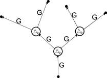
Figure 3. Factorization of $\Delta_{4}$

By well-ordering the non-leaf vertices of $\hat{\mathcal{T}}$ in any way such that the first vertex is attached to the root, and two consecutive vertices share an edge allows us to write this factorization in the style of the previous section.

$$\begin{CD}SL_{m}(\mathbb{C})@>{\Delta_{val(v_{1})-1}}>{}>SL_{m}(\mathbb{C})^{val{v_{1}}-1}@>{Id^{val(v_{1})-2}\times\Delta_{val(v_{2})-1}}>{}>SL_{m}(\mathbb{C})^{val(v_{1})+val(v_{2})-3}\ldots SL_{m}(\mathbb{C})^{n}\\ \end{CD}$$

This results in a direct sum decomposition of $\mathfrak{A}(\Delta_{n})$ into spaces $\mathcal{W}(\hat{\mathcal{T}},\lambda)$ indexed by assignments of dominant weights of $SL_{m}(\mathbb{C})$ to the edges of $\hat{\mathcal{T}}$, along with an assignment of $SL_{m}(\mathbb{C})-$linear maps at every vertex intertwining the corresponding tensor products of irreducible representations. From the introduction we know that the Plücker algebra is the subalgebra of $\mathfrak{A}(\Delta_{n})$ generated by the unique invariants $[\mathbb{C}\otimes\ldots V(\omega_{1}^{*})\otimes..\mathbb{C}]^{SL_{m}(\mathbb{C})}$ where $m$ of the $n+1$ pieces of the tensor product are copies of $V(\omega_{1}^{*})=\bigwedge^{m-1}(\mathbb{C}^{m}).$ The first piece, corresponding to the root, is always $\mathbb{C},$ and the other $n-m$ pieces are the trivial representation $\mathbb{C}.$ Each of these spaces is one dimensional, so we should be able to write down the tree diagram of a basis member for a chosen $\hat{\mathcal{T}}.$ To describe the diagram in general it is simplest to start with a rooted tree $\hat{\mathcal{T}}_{o}$ with $m$ leaves, give this tree an orientation as above. Each leaf of this tree is labeled with $\omega_{1},$ and to compute the representation labeling a given edge $e\in\hat{\mathcal{T}}_{o},$ simply count the number of leaves $n_{e}$ above $e$ with respect to the rooted orientation, and give it the label $\omega_{n_{e}}=\bigwedge^{n_{e}}(\mathbb{C}^{m}).$ Now dualize the whole picture, so $\omega_{i}$ becomes $\omega_{m-i}$. The result is shown below in Young tableaux.

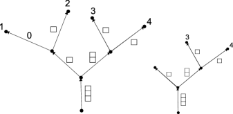
Figure 4. A tree weighted with representations

The root is labeled with $\bigwedge^{m}(\mathbb{C}^{m})$ which is trivial as an $SL_{m}(\mathbb{C})$ representation. In a general rooted tree $\hat{\mathcal{T}},$ take the convex hull of the root and the non-trivially labeled leaves. Combinatorially, this is the same as some rooted tree with $m$-leaves $\hat{\mathcal{T}}_{o},$ label the edges of $\hat{\mathcal{T}}$ accordingly, and label all other edges with the trivial representation. Note that up to scalars the available intertwiners $\bigwedge^{m-(i+j)}(\mathbb{C}^{m})\to\bigwedge^{m-i}(\mathbb{C}^{m})\otimes\bigwedge^{m-j}(\mathbb{C}^{m})$ in this diagram are all unique as expected. The subalgebra $\mathbb{C}[M_{m\times n}(\mathbb{C})]^{SL_{m}(\mathbb{C})}\subset\mathfrak{A}(\Delta_{n})$ is generated by the $\binom{n}{m}$ elements of this type. All diagrams are given explicitly in terms of the $m-1$ fundamental weights of $SL_{m}(\mathbb{C}),$ and one easily checks that an edge $e\in\hat{\mathcal{T}}$ is labeled nontrivially if and only if it is in the combinatorial convex hull of the $m$-nontrivially labeled leaves. Now consider the functional $H:X(T_{SL_{m}(\mathbb{C})})\to\mathbb{R}_{+}$ defined by $H(\omega_{k})=1$ for all fundamental weights $\omega_{k},$ and note that this functional gives the trivial representation the $0$ weight. Pick a non-negative length $d_{e}$ for edge $e\in\hat{\mathcal{T}},$ and consider the functional defined by assigning $d_{e}H$ to the edge $e.$ For the Plücker coordinate $Z_{i_{1}\ldots i_{m}}$ we have

(28) $$(\hat{\mathcal{T}},\vec{d}H)\circ(Z_{i_{1}\ldots i_{m}})=\sum_{e\in conv_{\hat{\mathcal{T}}}\{i_{1},\ldots,i_{m}\}}d_{e}\\$$

Proposition 3.1.

For any metric tree $(\mathcal{T},\ell)$ with $n$ leaves there is a rooted tree with $n$ leaves $\hat{\mathcal{T}}$, and a functional $\hat{h}$ with

(29) $$(\hat{\mathcal{T}},\hat{h})\circ(Z_{i_{1}\ldots i_{m}})=d_{i_{1}\ldots i_{m}}(\mathcal{T},\ell)$$

Proof.

To get $\hat{\mathcal{T}},$ one may add a root to $\mathcal{T}$ anywhere. It is simple to verify that this preserves combinatorial convex hulls. See figure 5 for an example. The root is added in the middle of an edge of $\mathcal{T},$ so in order to preserve the weighting information we must split the weight on this edge among the two new edges created by the addition of the root. The previous discussion does the rest. ∎

Figure 5. adding a root to the tree

This proposition establishes that we can replicate the $m$-dissimilarity vectors of a metric tree $(\mathcal{T},\ell)$ with branching filtrations. The efforts of the previous section confirm that branching filtrations always give tropical points. Together, these facts prove theorem 1.3.

4. Examples

In this section we will look at dissimilarity maps, Plücker coordinates, , and tree weighting functionals in more detail for a specific example. We will take a look at some elements and relations in the Plücker algebra $\mathbb{C}[Gr_{3}(\mathbb{C}^{8})].$ We choose a rooted tree with $8$ leaves, $\mathcal{T}$.

Figure 6. a rooted tree with 8 leaves

For simplicity we give $\mathcal{T}$ the metric where each edge has length $1,$ note that the corresponding unrooted tree would have one edge with length $2,$ and all others with length $1.$ We will find how $\mathcal{T}$ weights the Plücker relation

(30) $$Z_{123}Z_{456}-Z_{124}Z_{356}+Z_{125}Z_{346}-Z_{126}Z_{345}=0$$

in $\mathbb{C}[M_{3\times 8}(\mathbb{C})]^{SL_{3}(\mathbb{C})}.$ Each Plücker coordinate corresponds to an assignment of representations to the edges of $\mathcal{T}$, which are then weighted with the functional $H,$ as in figure 7.

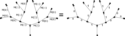
Figure 7. applying functional

In figure 8 we show the convex hulls of each set of leaves, rows correspond to Plücker monomials.

Figure 8. combinatorial convex hulls of leaves

This results in the following weights in the Plücker relation,

(31) $$t^{12}Z_{123}Z_{456}-t^{12}Z_{124}Z_{356}+t^{14}Z_{125}Z_{346}-t^{14}.Z_{126}Z_{345}=0$$

Next we look at the general case of $SL_{2}(\mathbb{C}).$ The $2$-dissimilarity vectors of a tree are the best understood dissimilarity vectors because of their association with the Grassmannian $Gr_{2}(\mathbb{C}^{n}),$ the same is true for $SL_{2}(\mathbb{C}^{n})$ branching algebras. The algebra $\mathfrak{A}(\Delta_{n})$ for $SL_{2}(\mathbb{C})$ is isomorphic to $\mathbb{C}[M_{2\times n+1}]^{SL_{2}(\mathbb{C})},$ indeed we have

(32) $$R(SL_{2}(\mathbb{C}))=Sym(V(\omega_{1}))\cong\mathbb{C}[x_{1},x_{2}]\\$$

It follows that the subalgebra of invariants $R(SL_{2}(\mathbb{C})^{n})^{SL_{2}(\mathbb{C})}$ is isomorphic to the $(2,n)$ Plücker algebra. For a rooted tree $\hat{\mathcal{T}},$ The functionals $(\hat{\mathcal{T}},\hat{h})$ are all given by assigning non-negative integers to the edges of $\hat{\mathcal{T}},$ as non-negative integers correspond to maps $h_{e}:C_{SL_{2}(\mathbb{C})}=\mathbb{Z}_{+}\to\mathbb{R}_{+}.$ Therefore for any metric tree $(\mathcal{T},\ell)$ we can construct a branching algebra filtration that weights the Plücker monomials the same as $(\mathcal{T},\ell).$ In this way, every member of the tropical Grassmannian $Trop(Gr_{2}(\mathbb{C}^{n}))$ is realizable by a branching filtration.

Christopher Manon:
Department of Mathematics,
University of California, Berkeley,
Berkeley, CA 94720-3840 USA,
chris.manon@math.berkeley.edu

References

- [AB] V. Alexeev and M. Brion, Toric degenerations of spherical varieties, Selecta Mathematica 10, no. 4, (2005), 453-478.
- [BC] C. Bocci and F. Cools, A tropical interpretation of -dissimilarity maps, Applied Mathematics and Computation Volume 212, Issue 2, 15 June 2009, Pages 349-356.
- [C] F. Cools, On the relation between weighted trees and tropical Grassmannians, Journal of Symbolic Computation Volume 44 , Issue 8 (August 2009), Pages: 1079-1086.
- [D] I. Dolgachev, Lectures on Invariant Theory, Longond Mathematical Society Lecture Note Series 296, Cambridge University Press, Cambridge, 2003.
- [FH] W. Fulton, J. Harris, Representation Theory, in: GTM, Vol. 129, Springer, Berlin, 1991.
- [G] B. Iriarte Giraldo, Dissimilarity Vectors of Trees are Contained in the Tropical Grassmannian, The Electronic Journal of Combinatorics 17, no 1, (2010).
- [Gr] F.D. Grosshans,Algebraic homogeneous spaces and invariant theory, Springer Lecture Notes, vol. 1673, Springer, Berlin, 1997.
- [M] C. Manon, The algebra of conformal blocks, http://arxiv.org/abs/0910.0577
- [M2] C. Manon. Graded valuations and tropical geometry, http://arxiv.org/abs/1006.0038
- [P] S. Payne, Analytification is the limit of all tropicalizations, Math. Res. Lett. 16, (2009) no 3, 543-556.
- [PSt] L. Pachter, and B. Sturmfels, Algebraic statistics for computational biology, Cambridge University Press, New York 2005
- [SpSt] D. Speyer and B. Sturmfels, The tropical Grassmannian, Adv. Geom. 4, no. 3, (2004), 389-411.