A new method to measure evolution of the galaxy luminosity function

Abstract

We present a new efficient technique for measuring evolution of the galaxy luminosity function. The method reconstructs the evolution over the luminosity-redshift plane using any combination of three input dataset types: 1) number counts, 2) galaxy redshifts, 3) integrated background flux measurements. The evolution is reconstructed in adaptively sized regions of the plane according to the input data as determined by a Bayesian formalism. We demonstrate the performance of the method using a range of different synthetic input datasets. We also make predictions of the accuracy with which forthcoming surveys conducted with SCUBA2 and the Herschel Space Satellite will be able to measure evolution of the sub-millimetre luminosity function using the method.

1 Introduction

A cornerstone of any working model of the formation of structure in the universe is knowledge of the galaxy luminosity function (GLF). The GLF is a measure of the comoving space density of galaxies per interval in luminosity. Determining how the GLF changes with cosmological epoch provides far-reaching insights into the processes that dictate the means by which galaxies form and evolve. This places strong statistical constraints on evolutionary theories, enabling determination of key characteristics such as the epoch of galaxy formation, merger rates, transformations between population types and the history of the universe’s global rate of formation of stars.

The value of measuring the evolution of GLFs has been appreciated for several decades and as such, many techniques have been employed to achieve this aim. Without any loss of generality, the GLF can be expressed as the local GLF scaled by an evolution function. The simplest and most direct method of estimating this evolution function is a model independent one where the GLF is measured at different epochs and compared with the local GLF. This provides a set of discrete estimates of the evolution at specific epochs. However, adopting a model-based procedure yields significant advantages. A well-proven approach is to assume the evolution function depends only on luminosity and redshift (see next section). For a given model of the evolution function chosen a priori, the best fit model is determined, subject to a set of observational constraints which contribute to different regions in the luminosity-redshift ($L-z$) plane. The virtue of model-based techniques is that a model consistent with all available observations can be used to make predictions by extrapolation into regions where data are sparse or lacking. Furthermore, a model can be used to identify those datasets whose improvement would most efficiently increase the constraints on the evolution function.

Model-based techniques are typically regarded as belonging to one of two types. Parametric evolution models adhere to some preconceived notion regarding the evolution of galaxies, for example, pure luminosity evolution or luminosity + density evolution (see Wall, Pope & Scott, 2008, and references therein for recent examples). Although an advantage of this type of modelling is that smooth functions are readily extrapolated, a major disadvantage is that the real evolution function may take on a very different form. So called ’free-form’ methods are not biased in this way and allow for a greater degree of flexibility over the $L-z$ plane when attempting to determine the evolution function.

Freeform techniques date back over three decades. Robertson (1978, 1980) developed an iterative freeform method to evaluate the evolution of the luminosity function for radio galaxies. The method was limited by allowing the evolution to vary only as a function of redshift (and not luminosity) and not giving a satisfactory indication of the range of solutions permitted by the observations. Peacock & Gull (1981) introduced a new method that incorporated luminosity dependence and measured the uncertainty on the evolution by considering the variation between different freeform model predictions. This improved technique saw successful application (e.g., Peacock, 1985; Dunlop & Peacock, 1990) although by the authors’ own admission, the full extent of the uncertainty still could not be verified by the range of models tested. Furthermore, the evolution function was modelled as a series expansion and the set of best-fit expansion coefficients determined by minimising $\chi^{2}$ using a non-linear search. This is both inefficient and does not guarantee that the global minimum has been found.

In this paper, we propose a new method, inspired by Peacock & Gull but offering some significant improvements. The method computes the evolution as a discretised (i.e., pixellised) function over the $L-z$. plane. This has the advantage that the evolution can be solved linearly, ensuring the best fit solution is always found with a single, highly efficient matrix inversion. Crucially, the full range of solutions permitted by the observations can be determined in a few simple extra computational steps. Despite being pixellised, we demonstrate how linear regularisation allows the evidence to be extrapolated into regions of the $L-z$ plane that are lacking data or where data are sparse. Finally, we show how the pixellisation can be adapted according to the constraints provided by the data.

The original motivation for this work was to investigate evolution of the luminosity function in the sub-millimetre (submm) waveband. The far-infrared (far-IR) and submm wavebands are particularly important for investigating the evolution of galaxies, not least because approximately half of the energy emitted by stars and active galactic nuclei since the big bang has been absorbed by dust and then re-radiated in these wavebands (Fixsen et al., 1998). In view of this, our interests lie in investigating not only the monochromatic luminosity functions at these wavelengths, but also the ‘dust luminosity function’, i.e., the space density of galaxies as a function of the total luminosity emitted by the dust in a galaxy.

Presently, observational data in the submm are particularly poor. However, this situation will begin to rapidly improve with the arrival of new submm instruments such as the second generation Submm Common User Bolometer Array (SCUBA2) and the Herschel Space Observatory (Herschel). Although the method we have developed is applicable to the luminosity function in any waveband, we describe and explore its use in this paper with an eye on its future application to forthcoming submm data.

In section 2 we present the method. Section 3 demonstrates the method with a range of synthetic datasets providing differing levels of constraints on the $L-z$ plane. Finally, we summarise in section 4 and discuss practical aspects of applying the method to real data.

2 The method

The overall aim of the method is to provide an estimate of the evolution of the GLF. We therefore write the GLF, $\phi$, as the product of the local GLF, $\phi_{0}$ and an evolution function, $E$:

$$\phi(L,z)=\phi_{0}(L)\,E(L,z)\,.$$ (1)

We have assumed that $E$ is a bivariate function of total far-IR/submm luminosity, $L$, and redshift, $z$. We work in terms of the bolometric luminosity rather than a monochromatic luminosity, in keeping with the traditions adopted in submm astronomy.

Until very recently, there were no direct submm measurements of $\phi_{0}$ (see Eales et al., 2009). Instead, the local GLF was estimated by extrapolating from shorter wavelength observations. In this way, the measurements had small statistical errors but, because of the uncertainty in the extrapolation, potentially large systematic errors. In what follows, we work towards determining $E$ directly, accepting the fact that in application to real submm data, $E$ potentially has systematic errors because of the uncertainty in $\phi_{0}$. Of course, it is a trivial exercise to re-write the formalism below in terms of $\phi(L,z)$ instead of $E(L,z)$ and use $\phi_{0}$ as an observational constraint. However, in order to determine $E$ from $\phi(L,z)$ obtained in this way, one would have to renormalise by $\phi_{0}$. This would therefore introduce the exact same systematic uncertainty on $E$ as that encountered by computing $E$ directly.

The crux of the method is to write $E$ as a discrete function, instead of the continuous form it has above. In this way, the evolution function takes on discrete values, $e_{j}$, in pixels which span the $L-z$ plane. As we show below, this discretisation turns the problem of determining $E$ into a more desirable linear one.

Observational constraints on $E$ can be categorised into three different types: number counts, galaxy redshifts and integrated background flux. Number count data provide the number of detected galaxies per unit area of sky binned by flux. The number of galaxies between two flux limits gives information about the integral of the luminosity function over an extended region of the $L-z$ plane, but does not provide information about whether the sources are luminous galaxies at high redshift or galaxies with low luminosity at low redshift in that region. Writing this in terms of the luminosity function, the expected number of detectable galaxies within a given flux bin $i$ is

$$n_{i}=\int^{z=\infty}_{z=0}{\rm d}V(z)\int^{L^{i}_{u}(z)}_{L^{i}_{l}(z)}{\rm d}L\,\phi(L,z)$$ (2)

where the lower and upper luminosity limits $L^{i}_{l}$ and $L^{i}_{u}$ correspond to the lower and upper flux limits of the bin and are therefore a function of redshift. These limits also depend on the frequency at which the flux is measured. Since $L$ is a bolometric luminosity, a frequency dependent correction must be applied to obtain the monochromatic rest-frame luminosity $L_{\nu}$ and hence observed flux $s_{\nu}(\nu_{o})=(1+z)L_{\nu}(\nu)/4\pi d_{L}^{2}$, where $\nu$ is the rest-frame frequency, $\nu_{o}=\nu/(1+z)$ is the observer frame frequency and $d_{L}$ is the luminosity distance. This correction is similar to a standard k-correction and depends on the galaxy spectral energy distribution (SED – see Section 3.1).

Using equations (1) and (2), the number of galaxies that contribute to $n_{i}$ from a given pixel $j$ in the $L-z$ plane can be written

$$m_{ij}\simeq e_{j}\,\int^{z^{j}_{u}}_{z^{j}_{l}}{\rm d}V(z)\int^{L^{ij}_{u}}_{L^{ij}_{l}}{\rm d}L\,\phi_{0}(L)\,=e_{j}\,a_{ij}\,.$$ (3)

Here, the volume integral is written assuming the $j$th pixel in the $L-z$ plane has fixed redshift boundaries. In general, the $L-z$ plane can be divided up into pixels of arbitrary geometry in which case the integral would extend over the portion of pixel $j$ that contributes to bin $i$. The luminosity limits are capped by the luminosity range spanned by pixel $j$, giving rise to zero contribution if they lie outside the pixel. Note also that the luminosity limits have picked up an additional index, reflecting their dependence on the redshift limits of pixel $j$. The approximation in equation (3) arises due to the fact that the continuous evolution implicit in equation (2) has been replaced by the discrete evolution $e_{j}$ which is assumed constant over the entire pixel. The discretised version of equation (2) can thus be written:

$$n_{i}=\sum_{j}\,m_{ij}\,,$$ (4)

where the sum acts over all pixels in the $L-z$ plane although only a fraction will typically contribute to number count bin $i$.

To incorporate redshift data, the procedure is essentially the same as for number counts. Redshift surveys provide the most direct measurement of the luminosity function at a specific place in the $L-z$ plane. Instead of binning galaxies by flux, and evaluating the integral in equation (2) over $0\leq z\leq\infty$, the data are binned by flux and redshift and the integral in equation (2) extends only over the redshift range of the bin. Instead of the quantities $a_{ij}$ defined in equation (3), an analogous set of quantities $b_{ij}$ are computed.

Including integrated background flux measurements requires a slightly different approach. Rather than compute the number of galaxies in a given data bin, the strength and spectral shape of the extragalactic background radiation in the far-IR/submm waveband puts a constraint on the integral of the luminosity-weighted GLF over the entire $L-z$ plane. The predicted integrated background flux, $f_{\nu}$, as measured at a given observer-frame frequency, $\nu_{o}$, is the sum of contributions from all galaxies over the whole $L-z$ plane, i.e.,

$$f_{\nu}(\nu_{o})=\int^{z=\infty}_{z=0}{\rm d}V(z)\int^{\infty}_{0}{\rm d}L\,\phi(L,z)\,s_{\nu}(\nu_{o})\,.$$ (5)

As before, the flux $s_{\nu}(\nu_{o})$ is computed allowing for the SED dependent correction that converts bolometric luminosity to monochromatic luminosity in the rest frame of the galaxy. Writing this equation in its discretised form gives

$$f_{\nu}(\nu_{o,i}) \simeq \sum_{j}e_{j}\,\int^{z^{j}_{u}}_{z^{j}_{l}}{\rm d}V(z)\int^{L^{ij}_{u}}_{L^{ij}_{l}}{\rm d}L\,\phi_{0}(L)\,s_{\nu}(\nu_{o,i})$$

$$= \sum_{j}e_{j}\,c_{ij}=f_{\nu,i}\,,$$

for the predicted integrated background flux measurement at the $i$th observer-frame frequency $\nu_{o,i}$.

From the observed galaxy number counts, $n^{o}_{i}$, the observed number counts binned by redshift, $n^{o}_{z,i}$ and the measured background flux, $f^{o}_{\nu,i}$ (all of which are assumed to be statistically independent of each other), the $\chi^{2}$ statistic in terms of the discretised predicted quantities is

$$\chi^{2}=\sum_{i=1}^{N_{1}}\frac{(n^{o}_{i}-\sum_{j}e_{j}\,a_{ij})^{2}}{\sigma_{i}^{2}}+\sum_{i=N_{1}+1}^{N_{1}+N_{2}}\frac{(n^{o}_{z,i}-\sum_{j}e_{j}\,b_{ij})^{2}}{\sigma_{i}^{2}}$$

$$+\sum_{i=N_{1}+N_{2}+1}^{N_{T}}\frac{(f^{o}_{\nu,i}-\sum_{j}e_{j}\,c_{ij})^{2}}{\sigma_{i}^{2}}=\sum_{i}\frac{(g_{i}-\sum_{j}e_{j}\,p_{ij})^{2}}{\sigma_{i}^{2}}\,.$$ (7)

In the above, there are $N_{1}$ number count bins, $N_{2}$ number counts binned by redshift, $N_{T}$ data points in total including the background flux measurements and the $\sigma_{i}$ are the 1$\sigma$ measurement errors. To simplify, the last term defines the general quantity $g_{i}$ as an observed data point and $p_{ij}$ refers to one of the corresponding quantities $a_{ij}$, $b_{ij}$ or $c_{ij}$. The set of values $e_{j}$ that minimise $\chi^{2}$ are those that satisfy $\partial\chi^{2}/\partial e_{k}=0$ which gives

$$\sum_{i}\,g_{i}\,p_{ik}/\sigma^{2}_{i}=\sum_{i}\sum_{j}\,e_{j}\,p_{ij}\,p_{ik}/\sigma_{i}^{2}\,.$$ (8)

By writing the vector element $d_{k}=\Sigma_{i}\,g_{i}\,p_{ik}/\sigma_{i}^{2}$ and the matrix element $M_{kj}=\Sigma_{i}\,p_{ij}\,p_{ik}/\sigma_{i}^{2}$, the solution to the set of linear equations in (8) can be written

$$\mathbf{e}=\mathbf{M^{-1}}\,\mathbf{d}\,,$$ (9)

where $\mathbf{e}$ is a vector containing the elements $e_{j}$.

In the presence of noise, the solution given by equation (9) is formally ill-conditioned and hence must be regularised. This is achieved by adding an extra term, the regularisation matrix $\mathbf{R}$, weighted by the regularisation weight, $\lambda$ (see Section 2.3):

$$\mathbf{e}=(\mathbf{M}+\lambda\mathbf{R})^{-1}\mathbf{d}\,.$$ (10)

The corresponding covariance matrix was derived by Warren & Dye (2003) for this problem:

$$\mathbf{C}=\mathbf{N}-\lambda\mathbf{N}(\mathbf{N}\mathbf{R})^{T}\,,\,\,\,\mathbf{N}=(\mathbf{M}+\lambda\mathbf{R})^{-1}.$$ (11)

This innocuous equation brings about the method’s key advantage over previous methods since the covariance matrix contains all of the information required to determine the uncertainty on the evolution function for a given set of model parameters (e.g., $\lambda$). The only extra step required to obtain the total error is to propagate the additional error that arises as a result of the uncertainty on the model parameters (see next section).

2.1 Bayesian Evidence

Although regularisation ensures that the solution given by equation (10) is well defined, it unfortunately introduces a new problem. Regularising a solution reduces the effective number of degrees of freedom by an amount that can not be satisfactorily determined. Furthermore, applying the same regularisation weight to two different models (for example different pixellisations of the $L-z$ plane) results in a different effective number of degrees of freedom for each model. This means the minimum $\chi^{2}$ is biased away from the most probable solution. More crucially, comparison between different models cannot be carried out fairly using the $\chi^{2}$ statistic. Therefore, $\chi^{2}$ can not be used to determine the most appropriate pixellisation given the observed data.

One solution to the problem is to simply not regularise. Fortunately, a better solution can be found by turning to Bayesian inference and ranking models by their Bayesian evidence instead of $\chi^{2}$. Suyu et al. (2006) derived an expression for the Bayesian evidence, $\epsilon$, for the linear inversion problem described by equation (10). Using the previous notation, this can be written

$$-2\,{\rm ln}\,\epsilon = \chi^{2}-{\rm ln}\,\left({\rm det}[\lambda\mathbf{R}]\right)+{\rm ln}\,\left({\rm det}[\mathbf{M}+\lambda\mathbf{R}]\right)$$ (12)

$$+\,\lambda\mathbf{e}^{T}\mathbf{R\,e}+\sum_{i}\,{\rm ln}(2\pi\sigma_{i}^{2})\,$$

with $\chi^{2}$ given by equation (2). Here, the covariance between all pairs of number count bins has been set to zero (i.e., it is assumed that all observed data points are independent of each other. For covariant data, the more general form given by Suyu et al., 2006, would be used).

The evidence is a probability distribution in the model parameters, allowing different models to be ranked fairly to find the most probable model. Formally, the evidence should be marginalised over all parameters and the resulting probability used in the ranking. However, Suyu et al. (2006) noted that a reasonable simplification is to approximate the evidence distribution as a delta function and use the maximum evidence directly to rank models (see the appendix of Dye et al., 2008, for more details). We have verified that this approximation is still valid for our application and hence have adopted it in the present study.

In our case, the evidence distribution is a function of two model parameters; the regularisation weight, $\lambda$, and a parameter, $\rho_{\rm thresh}$, described in the following section that controls the average size of adaptive pixels in the $L-z$ plane. Since the evolution depends on the value of these two parameters, their uncertainty, as given by the evidence distribution, must be included in the overall uncertainty on the evolution. For every $L-z$ plane pixel, we compute this additional uncertainty, $\sigma_{e}$, using:

$$\sigma_{e}^{2}=\sum_{j}\,\epsilon_{j}\,\Delta\rho_{\rm thresh}\,\Delta(\log\lambda)\,(e_{j}-<e>)^{2}$$ (13)

where the sum acts over all points on the grid spanned by $\lambda$ and $\rho_{\rm thresh}$ at which the evidence, $\epsilon_{j}$, is evaluated. Here, $\Delta\rho_{\rm thresh}$ and $\Delta(\log\lambda)$ is the separation between grid points along the $\rho_{\rm thresh}$ and $\log\lambda$ directions respectively and $<e>$ is the mean evolution in the pixel. Note also that the evidence must be normalised such that $\sum_{j}\,\epsilon_{j}\,\Delta\rho_{\rm thresh}\,\Delta(\log\lambda)=1$. This additional error is therefore effectively the scatter in the evolution, weighted by the evidence. We compute the overall error in the evolution as the quadrature sum of this error and the uncertainty given by the appropriate term in the covariance matrix given in equation (11).

2.2 Adaptive gridding of the $L-z$ plane

As we alluded to earlier, the $L-z$ plane can be pixellised in a completely general way. This has the advantage that smaller pixels can be placed in regions where there are superior observational data, i.e., higher signal-to-noise (S/N) and/or a higher density of data points. The effect of this is to better resolve the evolution function whilst maintaining an approximately constant level of constraints per pixel over the $L-z$ plane. Note that although the method prescribed by Peacock & Gull can adjust to the data by limiting the series expansion of the evolution function, this alters the global resolution over the plane, not in specific regions that are better constrained.

There are several criteria that could be used to control the size of pixels in the $L-z$ plane. One example would be to make direct use of the density of data points weighted by their S/N. Our criterion of choice is to use the covariance between pixel pairs provided by equation (11). Joining two pixels together increases the statistical independence and hence lowers the covariance of the resulting larger pixel with its neighbours. Defining a covariance threshold, $\rho_{\rm thresh}$, therefore introduces a criterion whereby pixel pairs whose covariance is larger than $\rho_{\rm thresh}$ are joined together.

The procedure we have used for adaptively gridding the $L-z$ plane is as follows:

• The $L-z$ plane is uniformly pixellised with a regular grid of small rectangular pixels. We tested a range of initial grid sizes and found that a $20\times 20$ grid is a good compromise between having sufficient resolution to properly adapt to the varying range of covariances over the $L-z$ plane and being of low enough resolution to maintain a high execution speed.

• For a given regularisation weight, the covariance matrix given by equation (11) is computed.

• The lower triangle of the covariance matrix is scanned for elements with an absolute value larger than the threshold covariance. Working from largest to smallest, pixel pairs whose covariance exceeds the threshold are joined. If, in working down the list, a pixel pair is encountered where one of the pixels has already been joined (because it had a higher covariance with another pixel), that pixel pair is skipped.

• New versions of the matrices $\mathbf{M}$ and $\mathbf{R}$ are computed taking into account the new pixellisation.

Steps 2) to 4) are repeated until the absolute value of all pixel covariances lie beneath the threshold $\rho_{\rm thresh}$. A more formally correct procedure would be to recompute the covariance matrix every time a pair of pixels are joined. This is considerably slower to execute in practice and we have found that the resulting adapted grid does not differ significantly from that produced by the faster procedure outlined above.

2.3 Regularisation

The regularisation matrix introduced in equation (10) arises as a result of adding a term to $\chi^{2}$ that becomes numerically smaller for smoother solutions. In this sense, regularisation behaves as a prior, acting to penalise noisy evolution functions. This is necessary to prevent ill-conditioning in equation (9). A potential disadvantage is that the evolution may not be smooth in reality so that regularisation biases the solution. However, the regularisation weight is set by the evidence which is maximised at the optimal value of the regularisation weight $\lambda$. If more data points are available, or if the data have a higher S/N, the evidence is maximised at a lower value of $\lambda$, allowing greater resolution of any sharp features in the reconstructed evolution. We have investigated this to an extent with a synthetic dataset produced using an evolution function with a cutoff (see Section 3).

The regularisation term added to $\chi^{2}$ can be written

$$\lambda B=\lambda\sum_{j,k}\,R_{jk}e_{j}\,e_{k}$$ (14)

where the $R_{jk}$ are the elements of the regularisation matrix $\mathbf{R}$. These depend on the regularisation scheme adopted as described below. This means that the solution remains linear since the partial derivative of $B$ with respect to the the $e_{j}$ is linear in $e$.

The simplest form of regularisation is zeroth order regularisation, where solutions that deviate from zero are penalised using $w_{jk}=\delta_{jk}$ so that $B=\sum_{j}\,e_{j}^{2}$. More useful forms of regularisation are first order schemes which penalise solutions that deviate from a constant and second order which penalise solutions that deviate from a gradient.

For most solutions, as we have found in carrying out the work presented herein, first and higher order regularisations give very similar results. Whilst we could implement first order regularisation, higher orders are generally more effective in terms of allowing more freedom in the solution. However, conventional higher order schemes are ill-defined on our adaptively gridded $L-z$ plane. For example, with a second order gradient scheme, pixel triplets required to form a finite difference second order derivative would be neither co-linear nor parallel. With this in mind, in this work, we have opted for a hybrid scheme that uses the difference between the evolution in a given pixel $j$ and the sum of evolutions in all neighbouring pixels $k$ weighted by

$$h_{jk}=(\Omega_{k}/\Omega_{j})\,N\exp(-y_{jk}^{2}/r^{2})\,.$$ (15)

Here, $\Omega$ is the area of the pixel in the $L-z$ plane, $y_{jk}$ is the separation of the centres of pixels $j$ and $k$ and $N$ is a normalisation constant set such that $\sum_{k,k\neq j}h_{jk}=1$ and $N=1$ when $j=k$. We set $r=1$ in units of pixels. The matrix $\mathbf{h}$ composed of elements given by equation (15) relates to the regularisation matrix $\mathbf{R}$ via $\mathbf{R}=\mathbf{h}^{T}\mathbf{h}$. By construction, $\mathbf{R}$ is non-singular so that the evidence given by equation (12) is always calculable.

As a final note, all regularisation weights quoted in this paper are scaled by the ratio of traces Tr$[\mathbf{M}$]/Tr$[\mathbf{R}]$. This normalisation factor means that the regularisation term $\lambda\mathbf{e}^{T}\mathbf{R\,e}$ and $\chi^{2}$ in equation (12) are weighted approximately equally when the scaled regularisation weight is unity.

2.4 Evidence maximisation procedure

There are two non-linear variables which must be adjusted when searching for the maximum evidence. These are the regularisation weight, $\lambda$ and the covariance threshold, $\rho_{\rm thresh}$. We also experimented with allowing the initial grid resolution to vary as a free parameter but found a strong degeneracy with $\rho_{\rm thresh}$ (if smaller pixels are used, more are joined to give a similar final adaptive grid).

With every trial set of $\lambda$ and $\rho_{\rm thresh}$, the procedure we have adhered to is:

• Form an adaptive grid (see Section 2.2).

• Form the regularisation matrix $\mathbf{R}$ for the current adaptive grid.

• Compute the matrix $\mathbf{M}$ and vector $\mathbf{d}$ as described in Section 2. From these, solve for the evolution as given by equation (10). We use an $LU$ factorisation routine with iterative refinement.

• Compute the covariance matrix as given by equation (11), $\chi^{2}$ given by equation (2) and then ${\rm ln}\,\epsilon$ from equation (12).

To find the maximum evidence, we performed a grid search over regularly stepped values of log$\lambda$ and $\rho_{\rm thresh}$. The nature of the adaptive gridding process is such that the evidence surface is not perfectly smooth. Despite smoothly varying $\lambda$ and $\rho_{\rm thresh}$, discontinuous jumps in the evidence occur when pixels are joined together. By choosing a smaller pixel grid, the size of the discontinuities are reduced. Our findings indicate that, provided the numerical evaluation of the integrals in equations (3) and (2) is precise, the evidence surface is sufficiently smooth with our chosen $20\times 20$ grid for easy identification the global maximum. In light of this, a more efficient automated search for the maximum such as a downhill simplex method could be used. In the results presented in the next section, we show contour plots of the evidence as a function of log$\lambda$ and $\rho_{\rm thresh}$.

3 Application to synthetic datasets

In this section, we demonstrate the method by applying it to synthetic datasets. These datasets are created from an input evolution function which can be compared with the reconstructed evolution functions.

3.1 Synthetic dataset construction

Three ingredients are required to synthesize a dataset:

• Dataset characteristics: In the case of number counts, these are the flux limits, in the case of number counts binned by redshift, the flux and redshift limits and for background flux measurements, the frequencies at which the flux is measured. In addition, all three types of dataset must stipulate a survey area for determination of uncertainties.

• The local luminosity function: To keep our demonstration reasonably realistic, we have used a luminosity function derived from local galaxies (selected with velocities $<30,000\,$km/s) in the Infra-Red Astronomical Satellite (IRAS) Point Source Catalogue of Saunders et al. (2000). In order to calculate the luminosity of each galaxy at each frequency of interest and to compute the bolometric luminosity, we estimated an SED. Each SED was fit to the 60 and 100$\,\mu$m IRAS flux and an estimate of the 850$\,\mu$m flux provided by the tight correlation between 60, 100 and 850$\,\mu$m flux reported by Vlahakis, Dunne & Eales . We refer the reader to a forthcoming study where we apply the method to real data (Dye et al., in preparation) for more details.

• The evolution function: We used two different evolution functions. The first is motivated by the findings of Heavens et al. (2004) and is a smooth function that monotonically increases with increasing redshift and luminosity. We used a bi-linear interpolation in $\log(1+z),\log L$ space according to $E(L,z)=1+xyE_{max}$ where $x={\rm log}_{10}(1+z)/{\rm log}_{10}(1+z_{max})$, $y=({\rm log}_{10}L)/{\rm log}_{10}(L_{max}/L_{min})$ and $E_{max}=1000$ is the maximum evolution at the point $(L_{max},z_{max})$ in the $L-z$ plane. The second model evolution function is the product of the first and an exponential cutoff $1.66\,e^{2-z}$ which applies at $z\geq 2$. The factor 1.66 ensures that the maximum evolution at $z=2$ is equal to 1000. The monotonic evolution function is defined over $0\leq z\leq 3$ whereas the cutoff function extends to $0\leq z\leq 5$. Both are defined over $10^{10}\leq L/L_{\odot}\leq 10^{13}$. Figure 1 plots the functions.

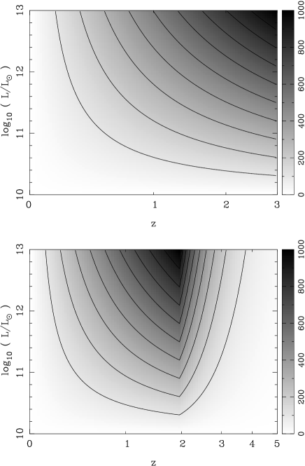
Figure 1: The two input evolution functions. Top: The monotonic function which increases with increasing redshift and luminosity. Bottom: The cutoff function formed by multiplying the monotonic function by an exponential cutoff $\propto e^{2-z}$ for $z\geq 2$. Contours in both plots are in intervals of 100.

In the case of number counts and number counts binned by redshift, we randomised the synthetic data according to Poisson statistics. Datasets were generated assuming either 0.1 deg² coverage (the ’low S/N’ case) or 10 deg² coverage (the ’high S/N’ case). Since background flux estimates are measured via a different means in practice, we have randomized the multi-frequency set of synthetic background fluxes with a 10% Gaussian error.

For all four combinations of S/N and evolution function, we have generated four different datasets:

• Number counts at 850$\,\mu$m between the limits 2 mJy (the confusion limit at 850$\mu$m with a 15 m dish) and 200 mJy in six flux bins equally spaced in log flux.

• Number counts at 850$\,\mu$m between the limits 0.1 and 200 mJy in 10 flux bins equally spaced in log flux.

• Number counts at 850$\,\mu$m between the limits 0.1 and 200 mJy in 10 intervals binned by 10 redshift intervals equally spaced in log($1+z$).

• A set of 10 background fluxes evaluated over the frequency range 2.4 THz - 300 GHz (125$\,\mu$m - 1 mm) at regularly spaced intervals in log(frequency).

Given currently available observing facilities, dataset C is somewhat unrealistic. Redshift measurements down to fluxes of $\sim 0.1\,\mu$mJy at 850$\,\mu$m are well below the confusion limit of 15m single dish observations and higher resolution interferometry presently lacks the sensitivity to generate large source samples. However, our choice to include this dataset is motivated by the fact that the dataset provides an indication of the best possible performance that can be expected from the method, thereby setting a benchmark for future surveys to aspire to.

The next section describes application of the reconstruction method to different combinations of these datasets. In addition to this, Section 3.2.4 outlines further tests of the method with a more realistic set of data based on what forthcoming Herschel and SCUBA2 surveys are expected to deliver.

3.2 Evolution reconstructions

We have applied our method to various dataset combinations to test how its performance depends on data availability and quality. The first and second groups of reconstructions in Sections 3.2.1 and 3.2.2 apply to datasets generated using the monotonic and cut-off evolution function respectively (see Figure 1). In the third group presented in Section 3.2.3, we compare recovery of the evolution with high S/N versions of datasets in the first and second groups. Finally, the last set of reconstructions in Section 3.2.4 are based on synthetic Herschel and SCUBA2 datasets.

3.2.1 Monotonic evolution

The first group of reconstructions are shown in Figure 2. These apply to the four dataset combinations A, A+D, B and C (see Section 3.1) generated using the monotonic evolution function in the low S/N case. The top row in the figure plots the coverage of each dataset in the $L-z$ plane. For each of the four test reconstructions shown, we have binned the input evolution function to the adaptive grid determined in each case to facilitate comparison with the recovered evolution. The binned input and recovered evolution is plotted in the second and third rows of the figure respectively. Comparing the two clearly shows that recovery of the input evolution becomes increasingly more faithful as the coverage of the datasets in the $L-z$ plane increases. The average size of adaptive pixels selected by the maximum evidence decreases with increasing coverage as a result of the increased constraining power of the data. Similarly, as the evidence contour plots at the bottom of the figure show, less regularisation of the evolution function is necessary when the data coverage is more extensive. Notice also that the covariance threshold at which the evidence is maximised is lower when the constraints provided by the data are greater. Finally, an important point to note is that in all cases, the significance of the residuals is distributed approximately normally with unit standard deviation. This means that the uncertainty on the evolution derived by our procedure is an accurate representation of where the recovered evolution truly differs from the input evolution.

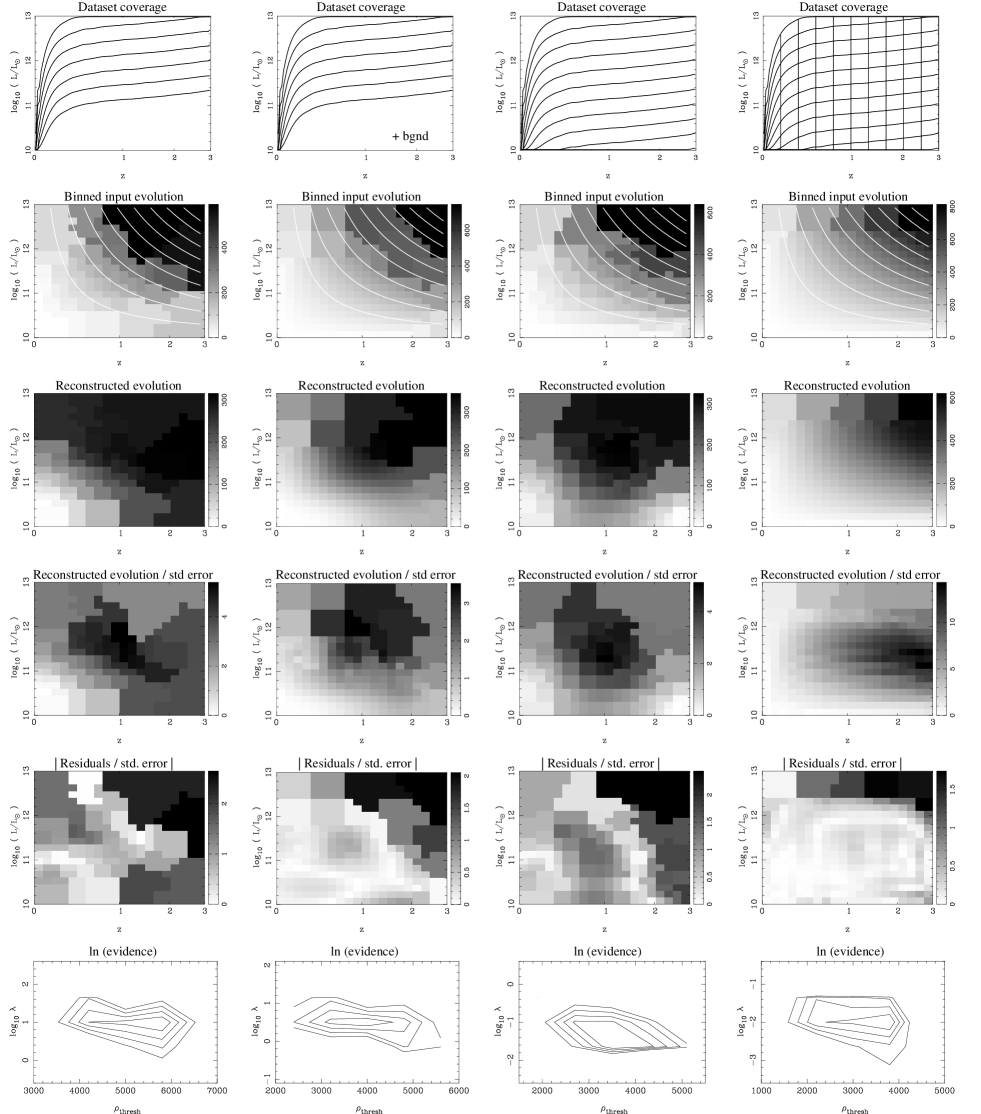
Figure 2: Application of the reconstruction method to four different combinations of low S/N datasets generated using the monotonic evolution function. Reading from left to right, columns correspond to datasets A, A+D, B, C (see Section 3.1). Reading from top to bottom, each row shows 1) coverage of input dataset(s), 2) input evolution function binned to the adaptive grid determined in the reconstruction (contours show the smooth underlying function plotted in Figure 1), 3) reconstructed evolution function, 4) the significance of the reconstructed evolution function, 5) the significance of the absolute residuals between the binned input and reconstructed evolution functions, 6) evidence contours in the plane spanned by covariance threshold and regularisation weight. Contours are stepped in four intervals of $\Delta\ln\epsilon=1$ away from the maximum.

The evidence contours show that a mild degeneracy exists between the covariance threshold and the regularisation weight. The degeneracy arises because a higher regularisation weight imposes stronger constraints on pixels. This has the effect of reducing their average covariance as quantified by equation (11). Therefore, at a fixed covariance threshold, as the regularisation weight increases, the average pixel size decreases. To maintain an optimal adaptive grid (i.e., an optimal average pixel size) at higher regularisation weights, a lower covariance threshold must be used and vice versa. In fact, the inclination of the evidence contours is parallel to lines of constant numbers of pixels. The maximum evidence therefore selects a specific subset of adaptive grids with approximately the same number of pixels from the set of all possible grids. The contours do not extend indefinitely because at the low covariance threshold end, the higher regularisation reduces the dynamic range of covariances over the $L-z$ plane. This results in an adaptive grid with more similarly sized pixels, i.e., the grid is not able to optimally adapt to the variation in data coverage. The reverse is true at the high covariance threshold end, where the lower regularisation results in a larger range of covariances to the extent that some pixels become too large while some remain too small to properly adapt to the data coverage.

Considering each reconstruction in turn in Figure 2, it is apparent that number count data alone are unable to recover the input evolution to a satisfactory accuracy. In the case of dataset A shown in the first column (with number counts that reach down to 2 mJy and no background flux measurements), the evolution is biased low at high $L$, high $z$ and biased high at high $L$, low $z$ and at low $L$, high $z$. This biasing occurs because the evolution function has been ’smeared’ over the $L-z$ plane by two effects. The first effect causes the evolution to be smeared along the lengths of flux bins. This is a direct result of the fact that the number of observed galaxies in a given bin can be reproduced by many different evolution profiles along the bin’s length, a point we will return to below. The second effect is that the regularisation effectively smooths the evolution. Regions of the $L-z$ plane where there are no constraints from the data are only constrained by the regularisation. In these regions, the evolution is extrapolated from neighbouring data-constrained regions, by an amount governed by the regularisation weight. This is a useful feature which we alluded to in the introduction: The ability to extrapolate is one of the key advantages of model-based approaches to measuring evolution.

It is apparent that the residuals in the first column of Figure 2 show that the most significant deviation from the input evolution occurs not where data constraints are lacking, but at high $L$, high $z$ where the evolution is strongest. This is again due to the smearing which causes a larger absolute difference when the evolution is stronger. In this sense, it could be argued that the method has performed more reliably in regions of the $L-z$ plane not covered by data. Of course this is primarily because the method assigns a much higher uncertainty to areas of zero coverage. The ratio of input to recovered evolution in areas of zero data coverage shows a stronger deviation from unity than areas that are covered by data.

Despite the biasing, the number count data still successfully detect a significant increase in the evolution from low $L$, low $z$ to high $L$, high $z$. At first sight, this seems incredible given that number count data contain nothing more than the number of galaxies between two flux limits. In other words, a single flux bin gives only a measure of the average evolution within it and nothing about the variation of the evolution. The same measured number of galaxies between two flux limits can be reproduced with a wide range of different evolution functions. Although true of an individual bin, this degeneracy becomes greatly reduced when other flux bins are added to the constraining data, especially when the solution is regularised.

Figure 3 illustrates the constraining power of pure number count data. We have plotted synthetic 850$\,\mu$m number counts generated using five different evolution functions covering $10^{10}\leq L/L_{\odot}\leq 10^{13}$ and $0\leq z\leq 3$ as in Figure 2. Four of these are monotonic and are simply the four 90-degree rotations of the previous monotonic function so that the maximum evolution is located at each of the four corners of the $L-z$ plane. The fifth evolution function was chosen to be a Gaussian with a full-width-at-half-max of $\Delta\log L=1$ and $\Delta z=1$, reaching the same maximum evolution but peaking in the centre of the $L-z$ plane.

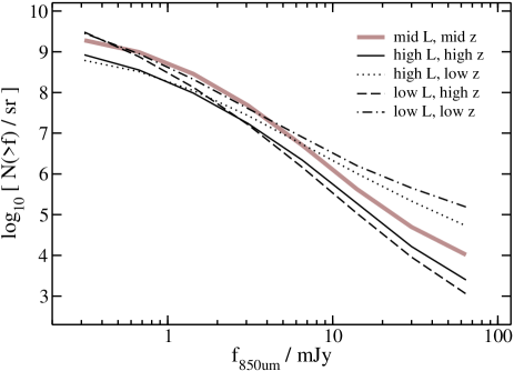
Figure 3: Synthetic 850$\,\mu$m cumulative number counts generated with five different evolution functions. Four of these are the four 90-degree rotations of the monotonic evolution function plotted in Figure 1 such that the maximum lies at each of the four corners of the $L-z$ plane. The fifth evolution function is described by a Gaussian with a full-width-at-half-max of $\Delta\log L=1$ and $\Delta z=1$, reaching the same maximum evolution but peaking in the centre of the $L-z$ plane. The counts arising from this fifth evolution function are shown by the broader grey line.

The figure shows that the four different monotonic evolution functions give rise to four unique number count datasets. All four datasets remain unique if any one undergoes the renormalisation $n(f)\rightarrow\alpha n(f)$ where $\alpha$ is a scale factor. This means that none of the four evolution functions can be renormalised to create a set of number counts that match those obtained using any of the other three evolution functions. Reversing this argument, the number count data can therefore distinguish between the four evolution functions. However, the Gaussian evolution function produces number counts which are very similar under renormalisation to the monotonic function that peaks at high $L$, high $z$ (compare the broader grey line with the thin continuous black line in Figure 3). This occurs because translating the Gaussian function by $\Delta z=+1.5$ along the direction of the 850$\,\mu$m flux bins (i.e., so that the peak lies at $z=3$), results in an evolution function that is very similar to the high $L$, high $z$ monotonic function. This serves to demonstrate the insensitivity of flux bins to variations in evolution along their length. The four rotated monotonic functions can be distinguished because they have moments perpendicular to lines of constant flux in the $L-z$ plane. Indeed, the reconstructed evolution obtained from the number counts generated using the Gaussian evolution function is very similar to the monotonic function which peaks at high $L$, high $z$, apart from a normalisation offset. Number counts can therefore not directly measure evolution cut-offs in redshift. We return to this point below.

The second column in Figure 2 shows the method applied to the combination of datasets A and D (i.e., 850$\,\mu$m number counts down to 2 mJy and 10 measurements of the background). Compared with just the number counts shown in the first column, it is clear that the reconstruction is more accurate. The added constraints from the background flux reduce the level of smearing. This is particularly apparent at low luminosity and high redshift where the biasing is much smaller. The additional constraints also enable a higher resolution reconstruction at low $L$, low $z$ and result in a lower required level of regularisation.

In the third column of Figure 2, we show how well the evolution is recovered with dataset B which comprises pure number count data again, but down to a lower flux limit of 0.1 mJy. In this case, the flux bins cover almost the entire $L-z$ plane. The figure shows that a similar, if not slightly higher level of biasing in the recovered evolution occurs, compared to that seen in the second column, due to the same smearing effects. However, there is an obvious improvement compared to the shallower number counts shown in the first column. This is apparent at low $L$ where the shallow counts permit a lower resolution reconstruction due to lack of coverage. Notice also that the solution requires a much lower level of regularisation.

A point to note is that the reconstructed evidence in regions of the $L-z$ plane constrained by data are not noticeably biased by regions that are not constrained by data. For instance, comparing the first and third columns of Figure 2 in the region of the $L-z$ plane covered by the brightest six flux bins shows that the recovered evolution and the significance of the residuals are very similar. Therefore, interpolation into areas lacking data coverage can be relied upon without detriment to the overall solution.

The fourth column of Figure 2 corresponds to the case where redshift information is included. Not surprisingly, the addition of redshifts improves the reconstruction dramatically by providing direct measurements of the evolution at specific points in the $L-z$ plane. The dataset allows reconstruction of the evolution on a much higher resolution grid. The larger pixels that still remain at high luminosities are due to increased Poisson noise caused by a significantly lower number density of galaxies (a common feature of most of the results shown in this paper). Despite the increased resolution, the significance of the reconstructed evolution is $\sim 3$ times higher compared to the cases where redshifts are not present. The solution is again biased most at high $L$, high $z$ where the evolution peaks and smearing has the largest effect, but this is less extensive and much reduced in magnitude.

3.2.2 Evolution with a cut-off

The second group of reconstructions apply to the four dataset combinations A, A+D, B and C (see Section 3.1) generated in this case using the cut-off evolution function with low S/N (i.e. assuming an area of 0.1 deg²). The top row in Figure 4 shows the coverage of the datasets over the $L-z$ plane which this time extends further in redshift out to $z=5$.

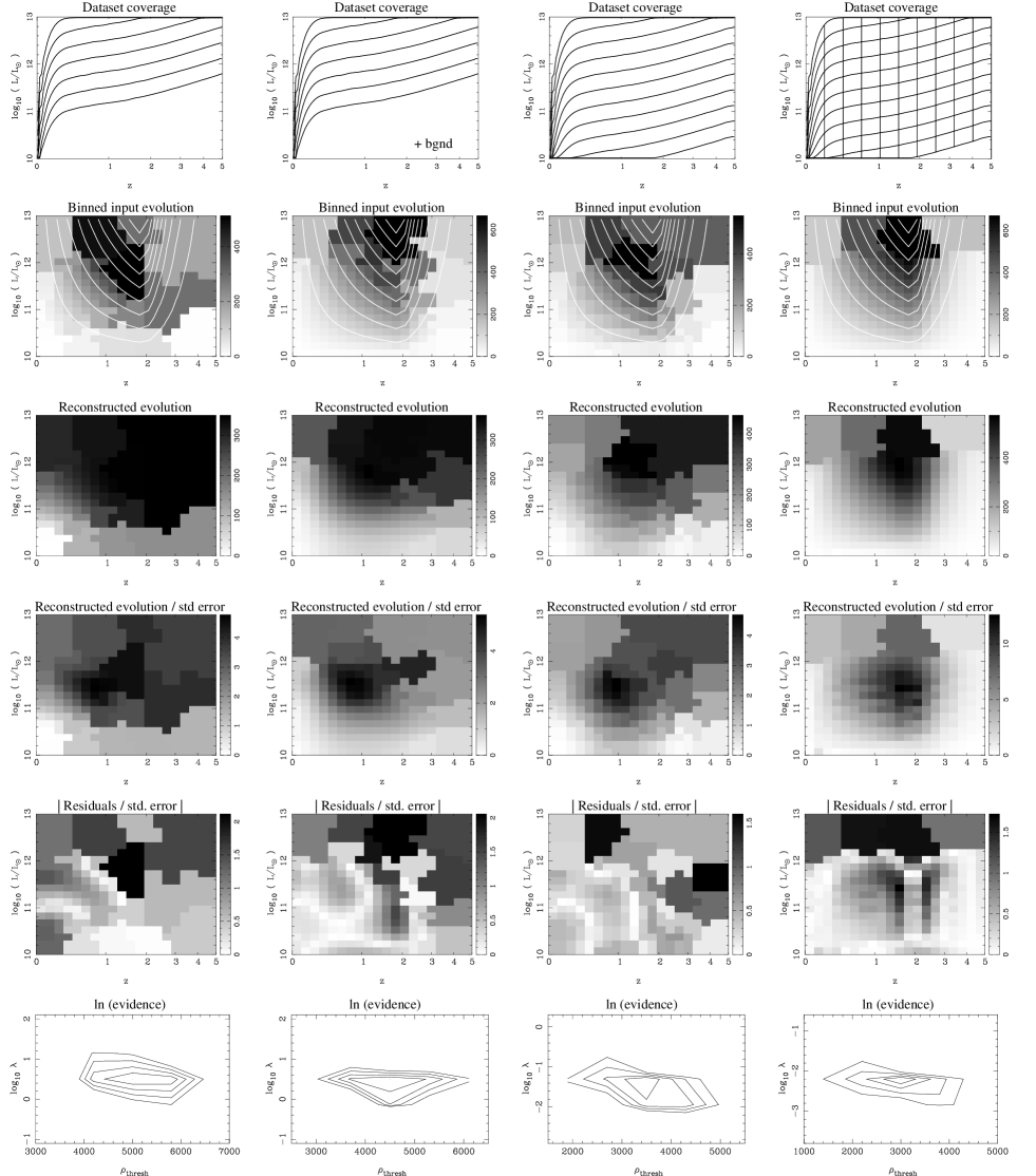
Figure 4: As Figure 2 but applied to low S/N datasets generated using the cut-off evolution function.

In terms of the variation of characteristics such as resolution, residuals, significance of the reconstructed evolution, optimal regularisation weights and optimal covariance thresholds, the reconstructions exhibit very similar traits to those seen with the previous group of datasets generated using the monotonic evolution function. However, there is one obvious and significant difference. Although the monotonic evolution function appears to be fairly well reconstructed without redshift information, the cut-off evolution function can not be properly recovered unless redshifts are included. Smearing along the length of flux bins removes any sign of the cut-off, pushing the strongest evolution to the highest redshift. This is the exact same behaviour observed previously with the ad-hoc Gaussian evolution function. We thus iterate again that redshift data is essential to measure any breaks or discontinuous features in the evolution.

We have investigated where, in relation to the break, redshift data most effectively constrains the break. Our findings show that redshift measurements lower than the break make little or no difference to identifying the location or even the existence of a break. Only redshift measurements at the break and beyond are able to constrain its location.

3.2.3 High S/N reconstructions

We have repeated some of the reconstructions carried out previously but with high S/N datasets (i.e. where an area of 10 deg² has been assumed). We generated the two extremes in datasets considered, namely the shallow number count only dataset and the deeper number counts binned by redshift, using both the monotonic and the cut-off evolution function. Figure 5 shows the results.

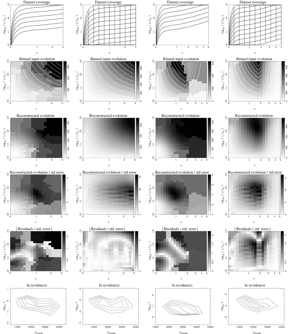
Figure 5: Application of the reconstruction method to high S/N datasets. The first and second columns correspond respectively to datasets A and C generated with the monotonic evolution function and the third and fourth columns to datasets A and C generated with the cut-off evolution. Row descriptions are the same as those in Figure 2.

Comparing with the corresponding low S/N reconstructions, the most striking difference is the improved resolution and higher significance of the reconstructed evolution. The rib-like structures present in the evolution significance (also seen to a lesser degree in the low S/N case) occur because of the varying number of constraints per pixel which range from one to four data bins depending on their alignment with the $L-z$ plane pixel grid.

An increase in the accuracy (i.e., a reduction in the average absolute size of the residuals) is also clear. Although the range of residual significances is approximately the same between high and low S/N datasets, the extent of the most significant discrepancies is less in the high S/N cases. In fact, the distribution of residual significances is slightly narrower than a normal distribution with unit $1\sigma$ width, implying that the errors are probably slightly over-estimated. If the residuals were randomly scattered over the $L-z$ plane, then this would imply that the evolution had been recovered to the best accuracy possible. However, the fact that the residuals form coherent patterns resembling the evolution function indicates that the reconstruction is not perfect. There are still low-level biases present, an inescapable consequence of regularisation.

3.2.4 Forthcoming survey predictions

The reconstructions previously considered give a good indication of how well different dataset types are able to constrain the evolution. From these simulations, it is clear that redshift data is vital to properly recover the input evolution. However, as we discussed in Section 3.1, the extent of the redshift data coverage in the $L-z$ plane was overly optimistic. Furthermore, in practice, observational data gathered for the purpose of measuring evolution will most likely be heterogeneous, comprising redshift and number count measurements from different studies observed at different wavelengths and to different depths.

In this section, we investigate the performance of the method with synthetic data generated to mimic a more realistic collection of data, typical of what might be expected from forthcoming submm surveys. Two of the largest datasets will be delivered by Herschel and SCUBA2. In the case of Herschel, we synthesized data based on the Spectral and Photometric Imaging Receiver (SPIRE) which operates in three passbands with central wavelengths 250, 350 and 500$\,\mu$m. For SCUBA2, we synthesized data at its longer wavelength channel at 850$\,\mu$m.

In terms of redshifts, we have assumed that measurements can be made down to the flux confusion limit at each wavelength. For SPIRE, these limits, as estimated by Lagache, Dole & Puget (2003), are approximately 10, 20 and 20 mJy at 250, 350 and 500$\,\mu$m respectively. The confusion limit for SCUBA2 at 850$\,\mu$m, is $\sim 2\,$mJy (e.g., Hughes et al., 1998). In terms of number counts, we have assumed that a flux limit $20\times$ lower than the confusion limit can be achieved using techniques such as the so-called ’P(D)’ statistical method (see, for e.g., Patanchon et al., 2009, and references therein) or to a lesser extent, exploitation of gravitational lens magnification (e.g., Smail, Ivison & Blain 1997 or more recently, Knudsen et al. 2006).

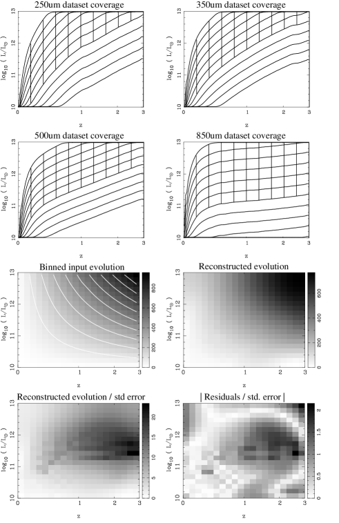
Figure 6: Application of the reconstruction method to simulated Herschel/SPIRE (250, 350 and 500$\,\mu$m) and SCUBA2 (850$\,\mu$m) data generated using the monotonic evolution function over 1 deg². The top four panels show the coverage of each dataset. In each case, redshift data extends down to the confusion limit and number counts reach down another factor of 20 in flux (see main text). The bottom four panels show the binned input evolution, the reconstructed evolution, the significance of the reconstructed evolution and the absolute significance of the residuals. The evidence in this case is maximised at $\rho_{\rm thresh}=2800$, log${}_{10}\,\lambda=-2.2$.

We tested the method with the synthetic data generated using the two different evolution functions as before. The top four panels of Figures 6 and 7 show the coverage of the datasets in the case of the monotonic and cut-off evolution function respectively. The redshift data cover the flux ranges 10 - 1000 mJy, 20 - 1000 mJy, 20 - 500 mJy and 2 - 200 mJy at 250, 350, 500 and 850$\,\mu$m respectively in six equal intervals in log($L$) and 10 equal intervals in log($1+z$). Similarly, the number count data cover four flux bins logarithmically spaced between the ranges 0.5 - 10 mJy, 1 - 20 mJy, 1 - 20 mJy and 0.1 - 2 mJy at 250, 350, 500 and 850$\,\mu$m respectively. We assumed an area of 1 deg².

The bottom four panels in Figure 6 show the reconstruction results for the monotonically evolving data. Despite a 10 times reduction in area and lower redshift data coverage of the $L-z$ plane compared with the high S/N case (shown in the second column of Figure 5), the input evolution is recovered with a comparable accuracy. At high luminosities, the average significance of the residuals is very similar to that in the high S/N case. This is not too surprising since the relative reduction in area is offset by the more numerous redshift data across the different wavelengths. Although the residuals fare worse at low luminosity where redshift data are completely lacking, they are smaller than the residuals that arise when no redshift data are present anywhere on the $L-z$ plane. For example, the residuals at low $L$, high $z$ in the third column of Figure 2 are higher and evaluated over larger pixels. The difference with the reconstruction using multi-wavelength data is that the variation of luminosity with redshift for a given flux changes as a function of observed wavelength. This is a direct result of the conversion between monochromatic and bolometric luminosity which depends on the SED assumed. The effect is that lines of constant flux, and therefore flux bins, in the $L-z$ plane corresponding to two different observed wavelengths can intersect each other. In the case of the reconstruction shown in Figure 6, some of the flux bins without redshift information cross other bins corresponding to different wavelengths where redshifts are present. Since data binned by both flux and redshift give a direct measure of the evolution at a specific location in the $L-z$ plane, this provides additional constraints on how the evolution must vary along the length of a flux-only bin.

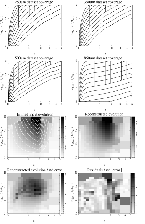
Figure 7: Application of the reconstruction method to simulated Herschel/SPIRE (250, 350 and 500$\,\mu$m) and SCUBA2 (850$\,\mu$m) data generated using the cut-off evolution function over 1 deg². Panels are as described in Figure 6. The evidence in this case is maximised at $\rho_{\rm thresh}=2700$, log${}_{10}\,\lambda=-2.8$.

Figure 7 shows how the method performs in reconstructing the simulated Herschel/SCUBA2 data generated using the cut-off evolution function. As in the case of the monotonically evolving data, the residuals exhibit a similar level of variation. However, unlike the monotonic case, the resolution of the recovered evolution is slightly lower than in the high S/N case. This is especially true at the highest redshifts where the evolution is considerably weaker than in the monotonic case. This results in much smaller numbers of galaxies per unit area of the $L-z$ plane and hence increased Poisson noise and covariance. The adaptive gridding procedure therefore increases the pixel size in these regions.

4 Summary

In this paper, we have presented a new method for measuring evolution of the galaxy luminosity function. The method computes the evolution as a discretised function of redshift and bolometric luminosity. The advantage brought about by this discretisation is that the evolution can be solved linearly, ensuring the best fit solution is always found with a single, efficient matrix inversion. Formulating this as a linear problem also brings the additional advantage that the uncertainty in the reconstructed evolution can be obtained with a few simple extra computational steps. Furthermore, by introducing linear regularisation, the evolution can be extrapolated into regions of the $L-z$ plane where data are lacking.

We have also developed a procedure for adaptively pixellising the evolution function. This allows the evolution to be reconstructed with higher resolution in regions of the $L-z$ plane where data constraints are stronger and lower resolution where constraints are weaker. The procedure uses the data to automatically set the optimal pixellisation via maximisation of the Bayesian evidence.

We have applied the method to a range of synthetic datasets constructed with two different input evolution functions; one rising monotonically with redshift and luminosity and the other incorporating a redshift cutoff. Comparing the reconstructed evolution with the input evolution provides a means of testing how well the method performs with varying dataset type, coverage and signal-to-noise. Our findings indicate that redshift measurements are essential to locate the presence of a cutoff in the evolution and that these must lie beyond the cutoff. Number count data alone allow for a surprisingly reasonable reconstruction if the evolution function is known to be monotonic, but falsely indicate monotonic behaviour when a redshift cutoff is present.

We have made predictions of the degree to which forthcoming submm surveys carried out with new instruments (SCUBA2 and Herschel) will allow evolution in the submm GLF to be determined. These simulations show that combining a mixture of number count data from both facilities and including measurements of redshifts down to the source confusion limit will allow for a very well resolved and reliable measurement of evolution. In particular, the predictions have demonstrated that much improved constraints are provided by pure number count data measured at a combination of different wavelengths, compared to counts measured at just one wavelength. This is a result of the cross-linking of flux bins on the $L-z$ plane due to the conversion between monochromatic and bolometric luminosity which is a function of both redshift and wavelength.

In terms of applying the method to real data, there are a few additional complexities that must be considered. One complexity is that real data are typically incomplete. This will result in the reconstructed evolution being a lower limit on the real evolution. Indeed, our simulations indicate that, due to regularisation, the reconstructed evolution tends to be underestimated even when the data are complete, although by an amount which is within the derived uncertainties. However, depending on the magnitude of the incompleteness, this may give rise to an underestimate that is not within the derived evolution error budget. In addition, depending on the level of regularisation, severe incompleteness in one dataset could significantly affect the reconstructed evolution in other areas of the $L-z$ plane covered by near-complete data.

Another consideration that must be made with real data is regarding the SED used for converting between monochromatic and bolometric luminosity. Clearly, if this is a poor match to the SEDs of the galaxies in a given dataset, then the assumed location of that dataset in the $L-z$ plane will be inaccurate and give rise to a systematic error in the recovered evolution. In the submm, this will be larger for fluxes near the peak of the observer-frame SED, but on average, should be a relatively small effect. Of course, instead of using a single SED as we have done in our simulations, source-specific SEDs, or dataset-specific SEDs could be used in practice.

In this paper, we have demonstrated the behaviour of the reconstruction method with a combination of different datasets and evolution functions. Although we have concentrated on key characteristics, there are many more that could have been tested. Since an exhaustive investigation of all configurations that might be encountered in practice is well beyond the scope of this work, a sensible approach would be to carry out simulations when applying the method to datasets that differ greatly from those tested here. In this way, any potential systematics that might arise from the data or any non-uniqueness in the reconstructed evolution could be quantified.

There are also several ways in which the method could be developed. For example, the adaptive pixellisation scheme is relatively simple and could be enhanced to offer greater adaptability. Another possible enhancement might be improving the use of redshift information. In this work, we incorporated redshifts by crudely binning number counts by redshift. This lowers the constraining power of the redshift data. With this in mind, we have begun development of a more sophisticated scheme that includes redshift information on a more efficient source by source basis. This will be presented in forthcoming work.

We are about to enter a new era in submm cosmology with the arrival of new instruments such as Herschel and SCUBA2. Surveys conducted with these instruments will give an increase in the number of detected submm sources of several orders of magnitude compared to existing surveys. Their significantly improved sensitivities will allow much wider ranges in luminosity and redshift to be explored. Combined with new methods to measure evolution, over the next few years, this will bring about a revolution in our overall understanding of how galaxies form and evolve.

Acknowledgements

SD acknowledges support by the Science and Technologies Facilities Council. We would like to thank the reviewer of this paper, Professor Steve Phillipps, for his helpful comments and suggestions.

References

- Dunlop & Peacock (1990) Dunlop, J. S. & Peacock, J. A., 1990, MNRAS, 247, 19
- Dye et al. (2008) Dye, S., 2008, MNRAS, 389, 1293
- Eales et al. (2009) Eales, S. A., et al., 2009, ApJ, 707, 1779
- Fixsen et al. (1998) Fixsen, D.J., Dwek, E., Mather, J.C., Bennet, C.L., Shafer, R.A., 1998, ApJ, 508, 123
- Heavens et al. (2004) Heavens, A. F., Panter, B., Jimenez, R., Dunlop, J., 2004, Nature, 428, 625
- Hughes et al. (1998) Hughes, D. H., et al., 1998, Nature, 394, 241
- Knudsen et al. (2006) Knudsen, K. K., Barnard, V. E., Van der Werf, P. P., Vielva, P., Kneib, J. -P., Blain, A. W., Barreiro, R. B., Ivison, R. J., Smail, I., Peacock, J. A., 2006, MNRAS, 368, 487
- Lagache, Dole & Puget (2003) Lagache, G., Dole, H. & Puget, J. -L., 2003, MNRAS, 338, 555
- Patanchon et al. (2009) Patanchon, G., et al., 2009, ApJ, in press, arXiv:0906.0981
- Peacock (1985) Peacock, J. A., 1985, MNRAS, 217, 601
- Peacock & Gull (1981) Peacock, J. A. & Gull, S. F., 1981, MNRAS, 196, 611
- Robertson (1978) Robertson, J. G., 1978, MRAS. 182, 617
- Robertson (1980) Robertson, J. G., 1980, MNRAS, 190, 143
- Saunders et al. (2000) Saunders, W., et al., 2000, MNRAS, 317, 55
- Smail, Ivison & Blain (1997) Smail, I., Ivison, R. J. & Blain, A. W., 1997, MNRAS, 490, L5
- Suyu et al. (2006) Suyu, S. H., Marshall, P. J., Hobson, M. P., Blandford, R. D., 2006, MNRAS, 371, 983
- (17) Vlahakis, C., Dunne, L. & Eales, S. A., 2005, MNRAS, 364, 1253
- Wall, Pope & Scott (2008) Wall, J. V., Pope, A. & Scott, D., 2008, MNRAS, 383, 435
- Warren & Dye (2003) Warren, S. J. & Dye, S., 2003, ApJ, 590, 673