1 String models for hadrons and composite strings.

An essential interest in string description of hadron interactions has arised as far back as forty years ago (the Nambu string [1] and dual resonance models initiated by Veneziano’s work [2]) due to the remarkable universal linearity of Regge trajectories $\alpha(t)$ for meson and baryon resonances [3] and [4]. $J=\alpha(M^{2})=\alpha(0)+\alpha^{\prime}_{H}M^{2}$ $(\alpha^{\prime}_{H}\approx 0.85\,$GeV${}^{-2})$; where J,M are spin and mass of a resonance. Now we have these trajectories up to $J=5$ and states for not only leading (n=0) but for second (n=1), for third (n=2) and even for fourth (n=3) daughter trajectories $J_{n}=\alpha(0)-n+\alpha^{\prime}_{H}M^{2}$ n=0,1,2,3… . See [4].

However attempts to build the string model for hadron interactions have not been succesful since consistent i.e. compatible with unitarity models for relativistic quantum strings [5],[6] have required the intercept of leading meson trajectory $\alpha(0)$ to be equal to one. A shift of this value from one has led to contradiction with unitarity since then states with negative norms have appeared. The leading $\rho$-meson trajectory has the intercept to be equal to one half approximately. Just this reason has led to superstring models for nonhadrons: for massless gluons (open strings) on the trajectory $J=1+\alpha^{\prime}_{P}M^{2}$ and for massless gravitons (closed strings) on the trajectory$J=2+1/2\alpha^{\prime}_{P}M^{2}$.

A generalization of classical multireggeon (multistring) vertices [7] has been suggested by author in 1993 [8] as a new solution of duality equations for many-string vertices in [7]. These string amplitudes have been used for description of interaction of many $\pi$-mesons [8]. New string vertices [9] give a new geometric picture for interactions of strings which has a natural description in terms of composite strings and three two-dimensional surfaces for moving open string instead of usual one. Additional edging two-dimensional surfaces carry quark quantum numbers (flavour, spin, chirality). This composite string construction reminds two similar other composite objects: a gluon string with two pointlike quarks at ends of it or simplest case of a string ending at two branes when they are themselves some strings. It is not surprisingly as we shall see further that we have here a possibility for N=3 extended superconformal Virasoro symmetry for open composite strings. Let us note that we have no supersymmetry in the Minkovsky (target) space for this model. The topology of interacting composite strings allows to solve the problem of the intercept $\alpha(0)$ for leading meson trajectory and to shift the value of this intercept to one half without breakdown of the extended superconformal Virasoro symmetry for composite strings due to non-vanishing conformal weights for fields on both edging two-dimensional surfaces.

2 Formulation of composite string model. Simple vertices for interacting composite strings.

We repeat here and in the following section formulations of vertices and generators of symmetries for the critical N=3 superconformal composite superstring model [9] with some corrections for formulation of supergauge generators $\widetilde{G}_{r}$ and hence for the critical condition.

For investigation of composite superstrings it is more appropriate to move from multi-string vertices to more simple vertices $\hat{V}_{i}$ corresponding to emission of ground states in an amplitude $A_{N}$ of interaction of N strings. In this case of composite superstrings operator vertices will contain additional ( to usual $\partial{X_{\mu}}$ and $H_{\mu}$ fields on the basic two-dimensional surface ) fields on edging surfaces : $Y_{\mu}$ and its superpartner $f_{\mu}$ with Lorentz indices $\mu$ = 0,1,2,3 . We include other edging fields ( J and its superpartner $\Phi$ ) which carry internal quantum numbers ( isospin and other flavour currents) on edging surfaces and similar I, $\Theta$ - fields on the basic two-dimensional surface. Since the edging fields are propagating only on the own edging surfaces it is convenient to introduce vacuum states for the fields on the separate edging surfaces and to write $A_{N}$ in equivalent form with help of these vacuum states:

$$A_{N}\!=\!\int\prod dz_{i}\langle 0^{(1,2)}|\hat{V}_{12}(z_{1})\langle 0^{(3)}|\hat{V}_{23}(z_{2})\times$$

$$\langle 0^{(4)}|\hat{V}_{34}(z_{3})|0^{(2)}\rangle\ \langle 0^{(5)}|...|0^{(i-1)}\rangle\ \hat{V}_{i,i+1}(z_{i})\times$$

$$\langle 0^{(i+2)}|...|0^{(N-2)}\rangle\ \hat{V}_{N-1,N}(z_{N-1})|0^{(N-1)}\rangle\ \times$$

$$\hat{V}_{N,1}(z_{N})|0^{(N,1)}\rangle\$$ (1)

This form(1) excludes this amplitude from the set of additive string models of the Lovelace’s paper [5] and leads to the topology of composite string models [8],[9]. Now we are ready to formulate the vertex operator $\hat{V}_{i,i+1}(z_{i})$ (Figure 1.) for this composite string model:

$$\hat{V}_{i,i+1}(z_{i})\ =\ z_{i}^{-L_{0}}\left[G_{r},\hat{W}_{i,i+1}\right]z_{i}^{L_{0}}\ ,$$

$$\hat{W}_{i,i+1}=\hat{R}^{out}_{i}\hat{R}_{NS}\hat{R}^{in}_{i+1}$$ (2)

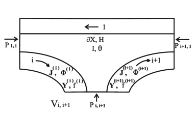
Figure 1:

The operators $\hat{R}^{out}_{i}$and $\hat{R}^{in}_{i+1}$ are defined by fields on i-th and (i+1)-th edging surfaces. The operator $\hat{R}_{NS}$ is defined by fields on the basic surface. They have the same structure as the operator $:\exp{ip_{i}X(1)}:$ of classical string models for both $Y$ and $J$ -fields:

$$\hat{R}^{out}_{i}=\exp{(\xi_{i}\sum_{n}\frac{J^{(i)}_{-n}}{n})}\ \exp{(k_{i}\sum_{n}\frac{Y^{(i)}_{-n}}{n})}\ \times$$

$$\exp{(ik_{i}Y^{(i)}_{0})}\widetilde{\lambda}^{(+)}_{i}\exp{(-k_{i}\sum_{n}\frac{Y^{(i)}_{n}}{n})}\ \times$$

$$\exp{(-\xi_{i}\sum_{n}\frac{J^{(i)}_{n}}{n})}\;$$ (3)

And we have the similar expression for $\hat{R}^{in}_{i+1}$:

$$\hat{R}^{in}_{i+1}=\exp{(-\xi_{i+1}\sum_{n}\frac{J^{(i+1)}_{-n}}{n})}\ \exp{(-k_{i+1}\sum_{n}\frac{Y^{(i+1)}_{-n}}{n})}\ \times$$

$$\exp{(-ik_{i+1}Y^{(i+1)}_{0})}\lambda^{(-)}_{i+1}\exp{(k_{i+1}\sum_{n}\frac{Y^{(i+1)}_{n}}{n})}\ \times$$

$$\exp{(\xi_{i+1}\sum_{n}\frac{J^{(i+1)}_{n}}{n})}\$$ (4)

$$\sum_{i}k_{i}=0$$ (5)

$$\hat{R}^{(NS)}_{i,i+1}=\exp{(-\zeta_{i,i+1}\sum_{n}\frac{I_{-n}}{n})}\ \exp{(-p_{i,i+1}\sum_{n}\frac{a_{-n}}{n})}\ \times$$

$$\exp{(-ip_{i,i+1}X_{0})}\Gamma_{i,i+1}\exp{(p_{i,i+1}\sum_{n}\frac{a_{n}}{n})}\ \times$$

$$\exp{(\zeta_{i,i+1}\sum_{n}\frac{I_{n}}{n})}\$$ (6)

Here we have introduced $\lambda_{\alpha}$ operators to be carrying quark flavours and quark spin degrees of freedom.

$$\langle 0|\widetilde{\lambda}^{(+)}=0;\lambda^{(-)}|0\rangle=0$$ (7)

$$\left\{\tilde{\lambda}_{\alpha}^{(-)},\lambda_{\beta}^{(+)}\right\}\ =\ \delta_{\alpha,\beta}\ ;\quad\tilde{\lambda}\ =\ \lambda T_{0},$$

$$T_{0}=\gamma_{0}\otimes\tau_{2}\ ;$$

$$\hat{p}_{i,i+1}=\hat{\beta}^{(i+1)}_{in}\hat{p}_{i+1}+\hat{\beta}^{(i)}_{out}\hat{p}_{i}=$$

$$\hat{\beta}^{(i+1)}_{in}k_{i+1}-\hat{\beta}^{(i)}_{out}k_{i}$$ (8)

$$\hat{\zeta}_{i,i+1}=\hat{\alpha}^{(i+1)}_{in}\hat{\xi}_{i+1}+\hat{\alpha}^{(i)}_{out}\hat{\xi}_{i}$$

$$\hat{\xi}_{i}=\widetilde{\lambda}^{(+)}_{i}\xi\lambda^{(-)}_{i};\$$ (9)

Here $\xi$ is some universal matrix over quark flavours. So we give some relation between of momenta (charges) which flow into the basic surface and into edging surfaces. Namely operators $\hat{\beta}(\hat{\alpha})$ define fractions of i-th and (i+1)-th momenta (charges) for the basic surface:

$$\hat{\beta}^{(i)}_{out}=\widetilde{\lambda}^{(+)}_{i}\beta_{out}\lambda^{(-)}_{i};$$

$$\hat{\alpha}^{(i)}_{out}=\widetilde{\lambda}^{(+)}_{i}\alpha_{out}\lambda^{(-)}_{i};$$ (10)

$$[\beta,\alpha]=0;\beta^{2}=\alpha^{2}=1$$ (11)

3 Extended Virasoro superconformal symmetries, supercurrent conditions and critical case for composite superstrings

Main symmetry of any string model is the superconformal symmetry to be defined by the Virasoro operators $G_{r}$. For composite superstring model we consider the set of states and of superconformal generators for the i-th section between the $\hat{V}_{i-1,i}$ vertex and $\hat{V}_{i,i+1}$ vertex in (1)(see Figure 2.).

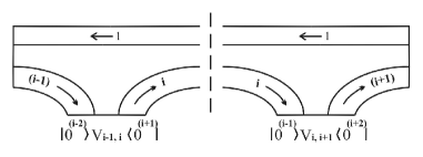
Figure 2:

Namely we have fields on (i-1), i, (i+1) edging surfaces :
$(Y^{(i-1)},f^{(i-1)});(J^{(i-1)},\Phi^{(i-1)})$;$(Y^{(i)},f^{(i)});(J^{(i)}$
$\Phi^{(i)})$; $(Y^{(i+1)},f^{(i+1)});(J^{(i+1)},\Phi^{(i+1)})$ fields

in addition to fields which are on the basic surface:
$(\partial{X},H)$;$(I,\Theta)$;

In order to consider our spectrum of states in more symmetric way regards left and right sides we introduce a set of auxiliary fields $(Y^{(a)},f^{(a)});(J^{(a)},\Phi^{(a)})$ instead of (i-1)-th and (i+1)-th fields in decomposition of 1 in the i-th section:

$$1=\sum|State(i-1,i,i+1)\rangle\ \langle State(i-1,i,i+1)|$$ (12)

Taking into account the operator $\langle 0^{(i+1)}|$ from the left side and operator $|0^{(i-1)}\rangle\$ from the right side we can replace (12) by the following sum:

$$\sum|State(i-1,i)\rangle\ \langle State(i,i+1)|=$$

$$\delta(fields(i-1)-fields(a))\sum|State(a,i)\rangle\ \times$$

$$\langle State(i,a)|\times\delta(fields(a)-fields(i+1))$$ (13)

Here we mean for $\delta(fields(i-1)-fields(a))$ (in the case of Y-fields):

$$\delta(Y(i-1)-Y(a))=$$ (14)

$$\sum_{[\lambda_{1},\lambda_{2},...]}\prod_{1}^{n}{\frac{(Y^{(i-1)}_{-n})^{\lambda_{n}}}{\sqrt{\lambda_{n}!}}}|0^{(i-1)}\rangle\ \langle 0^{(a)}|\prod_{1}^{n}{\frac{(Y^{(a)}_{n})^{\lambda_{n}}}{\sqrt{\lambda_{n}!}}}$$

and for $\delta(fields(a)-fields(i+1))$ correspondingly :

$$\delta(Y(a)-Y(i+1))=$$ (15)

$$\sum_{[\lambda_{1},\lambda_{2},...]}\prod_{1}^{n}{\frac{(Y^{(a)}_{-n})^{\lambda_{n}}}{\sqrt{\lambda_{n}!}}}|0^{(a)}\rangle\ \langle 0^{(i+1)}|\prod_{1}^{n}{\frac{(Y^{(i+1)}_{n})^{\lambda_{n}}}{\sqrt{\lambda_{n}!}}}$$

It is worth to note that the sets of states on the left and on the right of the vertex $\hat{V}_{i,i+1}$ will be the same ones that allows to connect corresponding decompositions unambiguously and to see independence on the number of the section for this consideration.

We shall consider this operator $\sum|State(a,i)\rangle\ \langle State(i,a)|$ which represents 1 in the Fock space for $|State(a,i)\rangle\$ and we shall extract spurious states in order to find the physical states spectrum.

Now superconformal generators $G_{r}$ can be defined as the following ones:

$$G_{r}=G^{Lor}_{r}+G^{Int}_{r}$$ (16)

$$G^{Lor}_{r}=\frac{1}{2\pi}\int\limits_{0}^{2\pi}d\tau[(H^{\mu}\frac{d}{d\tau}X_{\mu}+\hat{P}_{\nu}H^{\nu})+$$

$$(Y^{(a)}_{\mu}f^{(a)\mu}+\hat{p}_{1}f^{(1)}+Y^{(i)}_{\mu}f^{(i)\mu})]e^{-ir\tau}$$ (17)

$$G^{Int}_{r}\!=\!\frac{1}{2\pi}\int\limits_{0}^{2\pi}d\tau[(I\Theta+\xi_{1}\Phi^{(1)})+$$

$$(J^{(a)}\Phi^{(a)}+J^{(i)}\Phi^{(i)})]e^{-ir\tau}$$ (18)

Here we have a=i-1 (on the left side) or a=i+1 (on the right side). But unlike the Neveu-Schwarz model this composite string model has a new superconformal symmetry which defines by the following generators $\widetilde{G}_{r}$:

$$\widetilde{G}_{r}=\widetilde{G}^{Lor}_{r}+\widetilde{G}^{Int}_{r}$$ (19)

$$\widetilde{G}^{Lor}_{r}=$$ (20)

$$\frac{1}{2\pi}\int\limits_{0}^{2\pi}d\tau[\partial{X}_{\mu}\hat{\beta}^{(a)}f^{(a)\mu}+\partial{X}_{\mu}\hat{\beta}^{(i)}f^{(i)\mu}+$$

$$\hat{p}_{1}f^{(1)}+Y^{(a)}_{\mu}\hat{\beta}^{(a)}H^{\mu}+Y^{(i)}_{\mu}\hat{\beta}^{(i)}H^{\mu}-$$

$$(Y^{(a)}_{\mu}\hat{\beta}^{(a)}\hat{\beta}^{(i)}f^{(i)\mu}+Y^{(i)}_{\mu}\hat{\beta}^{(i)}\hat{\beta}^{(a)}f^{(a)\mu})]e^{-ir\tau}$$

$$\widetilde{G}^{Int}_{r}=\frac{1}{2\pi}\int\limits_{0}^{2\pi}d\tau[(I\hat{\alpha}^{(a)}\Phi^{(a)}+I\hat{\alpha}^{(i)}\Phi^{(i)})+$$

$$\xi_{1}\Phi^{(1)}+J^{(a)}\hat{\alpha}^{(a)}\Theta+J^{(i)}\hat{\alpha}^{(i)}\Theta-$$ (21)

$$(J^{(a)}\hat{\alpha}^{(a)}\hat{\alpha}^{(i)}\Phi^{(i)}+J^{(i)}\hat{\alpha}^{(i)}\hat{\alpha}^{(a)}\Phi^{(a)})]e^{-ir\tau}$$

The operators $\widetilde{G}_{r}$ give us the same commutation relations to the operator vertex $\hat{V}_{i,i+1}$ as $G_{r}$ ( here we have $a=i+1$ in $G_{r}$ and $\widetilde{G}_{r}$ ) :

$$[\widetilde{G}_{r},\hat{V}_{i,i+1}(1)]=[G_{r},\hat{V}_{i,i+1}(1)];$$

$$[\widetilde{G}_{r},\hat{W}_{i,i+1}]=[G_{r},\hat{W}_{i,i+1}]$$ (22)

Just here we have used the definite relations (8)-(11) for momenta and charges in the operator vertex $\hat{V}_{i,i+1}$. Taking into account the expressions (16)-(21) we can derive the corresponding commutation relations for $\widetilde{G}_{r}$ and $G_{r}$:

$$\{G_{r},G_{s}\}\ =\ 2L_{r+s}+\frac{D}{2}\left(r^{2}-\frac{1}{4}\right)\delta_{r,-s}$$ (23)

$$D=3d^{Lor}+3d^{Int}$$ (24)

$$\{G_{r},\widetilde{G}_{s}\}\ =2\widetilde{L}_{r+s};$$ (25)

here $d^{Lor}$ is the number of $Y$(or $X$)-components,
$d^{Int}$ is the number of $J$(or $I$)-components.

$$\{\widetilde{G}_{r},\widetilde{G}_{s}\}\ =4L_{r+s}-2\widetilde{L}_{r+s}+\frac{\widetilde{D}}{2}\left(r^{2}-\frac{1}{4}\right)\delta_{r,-s}$$ (26)

$$\widetilde{D}=6d^{Lor}+6d^{Int}$$ (27)

$$[L_{n},L_{m}]=(n-m)L_{n+m}+\frac{D}{8}n(n^{2}-1)\delta_{n,-m}$$ (28)

$$[L_{n},\widetilde{L}_{m}]=(n-m)\widetilde{L}_{n+m}$$ (29)

$$[\widetilde{L}_{n},\widetilde{L}_{m}]=2(n-m)L_{n+m}-(n-m)\widetilde{L}_{n+m}+$$

$$\frac{\widetilde{D}}{8}n(n^{2}-1)\delta_{n,-m}$$ (30)

$$[L_{n},G_{r}]=\left(\frac{n}{2}-r\right)G_{n+r}$$ (31)

$$[L_{n},\widetilde{G}_{r}]=\left(\frac{n}{2}-r\right)\widetilde{G}_{n+r}$$ (32)

$$[\widetilde{L}_{n},\widetilde{G}_{r}]=\left(n-2r\right)G_{n+r}-\left(\frac{n}{2}-r\right)\widetilde{G}_{n+r}$$ (33)

Due to this algebra and equations (22) we are able to prove as earlier in classical models that both $G_{r}$ and $\widetilde{G}_{r}$ operators generate spurious states. This commutation agebra allows to extract the independent combinations of operators $G_{r}$ and $\widetilde{G}_{r}$ which define the spectrum of spurious states. It is possible to extract the independent combinations of operators $G_{r}$ and $\widetilde{G}_{r}$ which define the spectrum of spurious states:

$$G^{I}_{r}=\frac{1}{3}(\widetilde{G}_{r}+2G_{r});G^{II}_{r}=(G^{Lor}_{r}-\widetilde{G}^{Lor}_{r});$$

$$G^{III}_{r}=(G^{Int}_{r}-\widetilde{G}^{Int}_{r})$$ (34)

Let us notice that our construction of vertices (2),(3)-(6) according to (8),(9) contains some definite combinations of fields with Lorentz indices:

$$k_{i}\widetilde{f}^{(i)}=k_{i}(f^{(i)}+\hat{\beta}_{i}H);$$

$$k_{i}\widetilde{Y}^{(i)}=k_{i}(Y^{(i)}+\hat{\beta}_{i}\partial X)$$ (35)

and with internal quantum numbers:

$$\zeta_{i}\widetilde{\Phi}^{(i)}=\zeta_{i}(\Phi^{(i)}+\hat{\alpha}_{i}\Theta);$$

$$\zeta_{i}\widetilde{J}^{(i)}=\zeta_{i}(J^{(i)}+\hat{\alpha}_{i}I)$$ (36)

Let us notice that all combinations (35) and (36) commute with operators $G^{II}_{r};G^{III}_{r}$.

Let us consider the construction of the spectrum generating algebra for this composite superstring by similar way as in classical string models [6]. For the given i- th section ( betweeen $V_{i-1,i}$ and $V_{i,i+1}$) we have fields on i,i-1,i+1 edging surfaces and fields on the basic surface. Spurious states for this basis are defined by products of operators $G^{I}_{r},G^{II}_{r},G^{III}_{r}$ and $L^{I}_{n},L^{II}_{n},L^{III}_{n}$. But only these states are not able to save from negative norms the spectrum of physical states as it has taken place for usual classical string models since the capacity of those of them which have negative norms is not enough. For the Fock space under consideration we can obtain states with negative norms not only as the powers of time components of the $\partial X$ and $H$ fields on the basic surface but as odd powers of other time-like components :$k_{a}\widetilde{f}^{(a)},k_{i}\widetilde{f}^{(i)}$ and $k_{a}\widetilde{Y}^{(a)},k_{i}\widetilde{Y}^{(i)}$.

Additional conditions for the composite string model are required in order to eliminate all negative norms from the spectrum of physical states. There is a simple solution for it. We shall require as gauge conditions the supercurrent conditions generated by $k_{i}\widetilde{f}^{(i)}$.

Namely we shall take the following constraints for our vertices:

$$[k_{i}\widetilde{Y}^{(i)}_{n},\hat{W}_{i,i+1}]=[\hat{W}_{i,i+1},k_{i+1}\widetilde{Y}^{(i+1)}_{n}]=0$$ (37)

Then we shall have enough states of negative norms generated by all gauge constraints. The equations (37) lead to the conditions:

$$k_{i}^{2}\rightarrow 0;k_{i+1}^{2}\rightarrow 0;(k_{i}k_{i+1})\rightarrow 0;$$ (38)

So our gauge supercurrents are independent and nilpotent ones:

$$[k_{i}\widetilde{Y}^{(i)}_{n},k_{i}\widetilde{Y}^{(i)}_{m}]=0;[k_{i+1}\widetilde{Y}^{(i+1)}_{n},k_{i}\widetilde{Y}^{(i)}_{m}]=0$$ (39)

Let us notice that our choice for additional gauge conditions is appropriate for emission of $\pi$-mesons (the case of usual quarks). It gives an explanation for massless $\pi$-mesons and correct amplitudes for $\pi$-mesons interaction [9]. But other quark flavours bring us to gauge supercurrent constrains which contain not only fields with Lorentz indices $\widetilde{Y}^{(i)}$ but and some part of fields $\widetilde{J}^{(i)}$ for internal quantum numbers. This part is vanishing for the case of usual $\pi$ - mesons.

Now we are able to build spectrum generating algebra (SGA) for our set of states in the same manner as for the Neveu- Schwarz string model in [6] with help of the operators of type of vertex operators (2) of the conformal spin j to be equal to one.

We shall use the light-like vectors $k^{(LI)}_{i}$ from our vertices ($(k^{(LI)}_{i})^{2}=0$) and consider a state of the generalized momentum $P^{(gen)}=p_{0}+Nk^{(LI)}_{i}$.

$$\frac{p_{0}^{2}}{2}=-1;(k^{(LI)}_{i})^{2}=0;(k^{(LI)}_{i}p_{0})=1$$

$$(k^{(LI)}_{i-1})^{2}=0;(k^{(LI)}_{i+1})^{2}=0;$$ (40)

$$(k^{(LI)}_{i}k^{(LI)}_{i+1})\rightarrow 0;(k^{(LI)}_{i}k^{(LI)}_{i-1})\rightarrow 0;$$

Transversal components of $k^{(LI)}_{i},p_{0}$ are vanishing $(p_{0})_{a}=(k^{(LI)}_{i})_{a}=0$. The generalized mass of this state is given by :

$$\frac{M^{(gen)2}}{2}=\frac{(p_{0}+Nk_{i}^{(LI)})^{2}}{2}=-1+N$$ (41)

We define the transversal operators of SGA as corresponding vertex operators.

All transversal SGA operators satisfy simple commutation algebra:

$$[(S^{(i)}_{a})_{n},(S^{(j)}_{b})_{m}]=m\delta^{i,j}\delta_{a,b}\delta_{m+n,0}$$

$$[(S^{(i)}_{a})_{n},(B^{(j)}_{b})_{r}]=0;$$

$$\{(B^{(i)}_{a})_{r},(B^{(j)}_{b})_{s}\}=\delta^{i,j}\delta_{a,b}\delta_{m+n,0}$$

So we can construct similarly to the DDF states transversal states $|Phys\rangle$ from powers of the transversal SGA operators:

$$|Phys\rangle=\prod{((S^{(i)}_{a})_{-n})^{\lambda(a,n)}}...|\Psi_{0}\rangle$$ (42)

These states satisfy all necessary gauge conditions.

Let us notice that all transversal SGA operators on the left side with (i-1)- and (i)- operators ( (i+1)-operators are vanishing there) can be defined with replacement of all (i)-fields to (i-1)-fields and vice versa of all (i-1)-fields to (i)-fields. It is true and for all transversal SGA operators on the right side with (i+1)- and (i)- operators ( (i-1)- operators are vanishing there ). They can be defined with replacement of all (i)-fields to (i+1)-fields and vice versa of all (i+1)-fields to (i)-fields. This possibility to reformulate these sets of states allows to move from states of i-th section under consideration to states in (i-1)-th section and so on. Hence our consideration can be carried out up to ends of our amplitude (1) and does not depend on the number i of this section.

Moving from these DDF type states to arbitrary states we can obtain them as usually with help of ordered powers of the conformal generators $G^{I}_{r},L^{I}_{n};_{n};G^{II}_{r},L^{II}_{n};G^{III}_{r},L^{III}_{n}$ and of powers of the supercurrent operators
$k^{(LI)}_{i}\widetilde{Y}^{(LI)(i)}$, $k^{(LI)}_{i}\widetilde{f}^{(LI)(i)}$ acting on $|Phys\rangle$ states:

$$(G^{I}_{\frac{-1}{2}})^{\lambda(1)}(G^{I}_{\frac{-3}{2}})^{\lambda(3)}...(L^{I}_{-1})^{\mu(1)}(L^{I}_{-2})^{\mu(2)}...$$

$$\prod_{r}(k^{(LI)}_{i-1}\widetilde{f}^{(LI)(i-1)}_{-r})^{\gamma(i-1,r)}$$

$$\prod_{n}(k^{(LI)}_{i-1}\widetilde{Y}^{(LI)(i-1)}_{-n})^{\delta(i-1,n)}$$

$$\prod_{r}(k^{(LI)}_{i}\widetilde{f}^{(LI)(i)}_{-r})^{\gamma(i,r)}$$

$$\prod_{n}(k^{(LI)}_{i}\widetilde{Y}^{(LI)(i)}_{-n})^{\delta(i,n)}|Phys\rangle$$ (43)

Then we can repeat considerations in the Neveu-Schwarz model [6]] for the theorem about absence of ghosts in the spectrum of physical states in our case for the critical value of the number of effective dimensions and taking into account the conditions (40).

In critical case the operators $G^{I}_{\frac{1}{2}}$ and

$$G^{I}_{\frac{3}{2}}+2(G^{I}_{\frac{1}{2}})^{3}=$$

$$=G^{I}_{\frac{3}{2}}+\frac{2}{3}(\widetilde{G}_{\frac{1}{2}}+2G_{\frac{1}{2}})(\widetilde{L}_{1}+2L_{1})=G^{\prime I}_{\frac{3}{2}}$$ (44)

define null states:

$$\{G^{\prime I}_{\frac{3}{2}},G^{I}_{\frac{-1}{2}}\}=0$$ (45)

$$|S_{\frac{-3}{2}}\rangle=G^{\prime I}_{\frac{-3}{2}}|Phys\rangle;\langle S_{\frac{3}{2}}|S_{\frac{-1}{2}}\rangle=0$$ (46)

$$|S_{\frac{-1}{2}}\rangle=G^{I}_{\frac{-1}{2}}|Phys\rangle;\langle|S_{\frac{1}{2}}|S_{\frac{-1}{2}}\rangle=0$$

$$\langle|S_{\frac{3}{2}}|S_{\frac{-3}{2}}\rangle=0$$ (47)

The critical case corresponds to the condition (46). It requires the condition (47) to be satisfied:

$$L_{0}=\widetilde{L}_{0}=\frac{1}{2}$$ (48)

and definite values of numbers of fields:

$$d_{crit}=2d^{Lor}+2d^{Int}=10$$ (49)

For the critical case we can prove by the same way as in the Neveu-Schwarz model that the norms of all physical states are nonnegative if all constraints for physical states are fulfilled. That means four fields for all Y-fields i.e. $Y^{(i)}_{\mu},\mu=0,1,2,3$ and one component for $J^{(i)}$-fields.

4 Hadron vertices for u,d,s quark flavours in tree hadron amplitudes

Let us consider simple composite critical superstring vertices for usual u,d and s quark flavours in arbitrary tree amplitudes.

Our choice for $\pi$-meson emission vertex coincides with the simplest vertex (2)-(6)

with $k_{i}^{2}=k_{i+1}^{2}=\mu^{2}$;$k_{i}k_{i+1}=0$ and $\mu^{2}\rightarrow 0$ . The last conditions provide the supercurrent conditions (38) and leads to $m_{\pi}^{2}=0$.

We can propose some simple choice for $\beta_{in},\beta_{out}$:

$$\beta_{in}^{(i+1)}=a\frac{\hat{k}_{i+1}}{\mu}+b\gamma_{5};\beta_{out}^{(i)}=a\frac{\hat{k}_{i}}{\mu}-b\gamma_{5};$$

$$a=\cos{\phi};b=\sin{\phi};$$ (50)

Let us notice that value of $\phi$ defines the fraction of momentum to be flowing into two-dimensional surface for the closed string sector and therefore $\phi^{2}\sim 10^{-38}$. As it is proposed $\lambda^{(-)}_{i+1}$ and $\lambda^{(+)}_{i}$ are eigenfunctions of operators $\hat{\beta_{in}^{(i+1)}}$ and $\hat{\beta_{out}^{(i)}}$ correspondingly :

$$\hat{\beta_{out}^{(i)}}\lambda^{(+)}_{(\eta_{i})}|0\rangle=\eta_{i}\lambda^{(+)}_{(\eta_{i})}|0\rangle;\eta_{i}=\pm 1$$ (51)

$$\langle 0|\widetilde{\lambda}^{(-)}_{(\eta_{i+1})}\hat{\beta_{in}^{(i+1)}}=\eta_{i+1}\langle 0|\widetilde{\lambda}^{(-)}_{(\eta_{i+1})};\eta_{i+1}=\pm 1$$ (52)

So we have the following $\pi$- meson emission vertex:

$$\hat{V}_{i,i+1}(z_{i})\ =\ z_{i}^{-L_{0}}\left[G_{r},\hat{W}_{i,i+1}\right]z_{i}^{L_{0}}\ ,$$

$$\hat{W}_{i,i+1}=\hat{R}^{out}_{i}\hat{R}_{NS}\hat{R}^{in}_{i+1}$$ (53)

$$\hat{R}^{out}_{i}=$$

$$\exp{(\xi_{i}\sum_{n}\frac{J^{(i)}_{-n}}{n})}\ \exp{(k_{i}\sum_{n}\frac{Y^{(i)}_{-n}}{n})}\ \times$$

$$\exp{(ik_{i}Y^{(i)}_{0})}\widetilde{\lambda}^{(+)}_{i}\exp{(-k_{i}\sum_{n}\frac{Y^{(i)}_{n}}{n})}\ \times$$

$$\exp{(-\xi_{i}\sum_{n}\frac{J^{(i)}_{n}}{n})}\;$$ (54)

$$\hat{R}^{in}_{i+1}=$$

$$\exp{(-\xi_{i+1}\sum_{n}\frac{J^{(i+1)}_{-n}}{n})}\ \exp{(-k_{i+1}\sum_{n}\frac{Y^{(i+1)}_{-n}}{n})}\ \times$$

$$\exp{(-ik_{i+1}Y^{(i+1)}_{0})}\lambda^{(-)}_{i+1}\exp{(k_{i+1}\sum_{n}\frac{Y^{(i+1)}_{n}}{n})}\ \times$$

$$\exp{(\xi_{i+1}\sum_{n}\frac{J^{(i+1)}_{n}}{n})}\$$ (55)

$$\hat{R}^{(NS)}_{i,i+1}=$$

$$\exp{(-\zeta_{i,i+1}\sum_{n}\frac{I_{-n}}{n})}\ \exp{(-p_{i,i+1}\sum_{n}\frac{a_{-n}}{n})}\ \times$$

$$\exp{(-ip_{i,i+1}X_{0})}\Gamma_{i,i+1}\exp{(p_{i,i+1}\sum_{n}\frac{a_{n}}{n})}\ \times$$

$$\exp{(\zeta_{i,i+1}\sum_{n}\frac{I_{n}}{n})}\$$ (56)

We require $\xi_{i}^{2}=\xi_{i+1}^{2}=\frac{1}{2}$ in order to have the conformal spin of this vertex to be equal to one.

The product $\widetilde{\lambda}^{(+)}_{(\eta_{i})}...\Gamma_{i,i+1}...\lambda^{(-)}_{(\eta_{i+1})}$ can be presented for the $\pi$- meson emission vertex in the following way:

$$\widetilde{\lambda}^{(+)}_{\beta,(\eta_{i})}...\Gamma_{i,i+1}...\lambda^{(-)}_{\alpha,(\eta_{i+1})}=$$

$$\sum_{\eta_{i},\eta_{i+1},\alpha,\beta}\widetilde{\lambda}^{(+)}_{\beta,(\eta_{i})}...\epsilon_{\eta_{i},\eta_{i+1}}\tau^{\pi(ij)}_{\beta\alpha}...\lambda^{(-)}_{\alpha,(\eta_{i+1})}$$ (57)

Here $\beta;\alpha=1,2$ are isotopic indices and $\tau^{\pi(ij)}$ is a corresponding isotopic Pauli matrix.

For $A_{4}$ we have from (1)

$$A_{4}\!=\!\int\prod dz_{i}\langle 0^{(1,2)}|\hat{V}_{12}(z_{1})\langle 0^{(3)}|\hat{V}_{23}(z_{2})\times$$

$$\langle 0^{(4)}||0^{(2)}\rangle\ \hat{V}_{3,4}(z_{3})|0^{(3)}\rangle\ \hat{V}_{4,1}(z_{4})|0^{(4,1)}\rangle\$$ (58)

For $\pi+\pi\rightarrow\pi+\pi$ we have

$$A_{4}=g^{2}\int_{0}^{1}dxx^{-\frac{3}{2}}x^{(-\frac{p_{13}^{2}}{2}+\frac{\xi_{1}^{2}}{2}+\frac{\xi_{3}^{2}}{2}-\frac{k_{1}^{2}}{2}-\frac{k_{3}^{2}}{2}+\frac{\zeta_{13}^{2}}{2})+\frac{1}{2}}$$

$$(1-x)^{-p_{23}p_{34}+\zeta_{23}\zeta_{34}+k_{3}^{2}-\xi_{3}^{2}-1}$$ (59)

$$(-p_{23}p_{34}+\zeta_{23}\zeta_{34}+k_{3}^{2}-\xi_{3}^{2})Tr(\Gamma_{12}\Gamma_{23}\Gamma_{34}\Gamma_{41})$$

So we obtain this amplitude as a simple beta function

$$A_{4}=g^{2}\frac{\Gamma(1-\alpha^{t}_{0}-\frac{1}{2}t)\Gamma(1-\alpha^{s}_{0}-\frac{1}{2}s)}{\Gamma(1-\alpha^{t}_{0}-\frac{1}{2}t-\alpha^{s}_{0}-\frac{1}{2}s))}$$

$$Tr(\Gamma_{12}\Gamma_{23}\Gamma_{34}\Gamma_{41})$$ (60)

with $t=p_{13}^{2},s=p_{34}^{2};$
$\alpha^{t}_{0}=1-\frac{\xi_{1}^{2}}{2}-\frac{\xi_{3}^{2}}{2}+\frac{k_{1}^{2}}{2}+\frac{k_{3}^{2}}{2}-\frac{\zeta_{13}^{2}}{2});$
$\alpha^{s}_{0}=-\frac{p_{23}^{2}}{2}+\frac{p_{34}^{2}}{2}-\zeta_{23}\zeta_{34}-k_{3}^{2}+\xi_{3}^{2}$;

$k_{i}^{2}=0$;$\xi_{i}^{2}=\xi^{2}=\frac{1}{2}$ and hence $\zeta_{13}=\xi_{1}+\xi_{3}=0,\zeta_{23}=\zeta_{34}=0$; $p_{23}^{2}=p_{34}^{2}=m_{\pi}^{2}=0$
and $\alpha^{t}_{0}=\alpha^{s}_{0}=\frac{1}{2}$

After this natural choice for the $\pi$- meson emission vertex we can not build the K- meson emission vertex similarly without a lost of the supercurrent conditions (37) for the s-quark edging surface and hence with the breakdown of our construction of the spectrum generating algebra and then with appearance of states of negative norms in the physical spectrum.

But it is possible to move to another form for $\hat{W}_{i,i+1}$ in the case of K-mesons without a lost of the supercurrent conditions:

$$\hat{V}_{i,i+1}(z_{i})\ =\ z_{i}^{-L_{0}}\{G_{r},\widetilde{W}_{i,i+1}\}z_{i}^{L_{0}}\ ,$$

$$\widetilde{W}_{i,i+1}=\left[G_{r},\hat{W}_{i,i+1}\right]$$ (61)

$$\hat{W}_{i,i+1}=\hat{R}^{out}_{i}\hat{R}_{NS}\hat{R}^{in}_{i+1}$$

Here we have i-th edging surface for usual (u,d) quark flavours with $k_{i}^{2}=\mu^{2}$;$k_{i}k_{i+1}=0;\mu^{2}\rightarrow 0$;$\xi_{i}^{2}=\frac{1}{2}$ and i+1-th edging surface for s-quark flavour.

There are two orthogonal light-like supercurrent conditions: the old one

$$k_{i}\widetilde{f}^{(i)}=k_{i}(f^{(i)}+\hat{\beta}_{i}H);$$

$$k_{i}\widetilde{Y}^{(i)}=k_{i}(Y^{(i)}+\hat{\beta}_{i}\partial X)$$ (62)

and the second one

$$\widetilde{f}_{s}=k_{i+1}(f^{(i+1)}+\hat{\beta}_{i+1}H)-\xi_{i}\Phi^{(i)}$$

$$+\xi_{i+1}\Phi^{(i+1)}+(\xi_{i+1}\hat{\alpha}_{i+1}-\xi_{i}\hat{\alpha}_{i})\Theta;$$

$$\widetilde{Y}_{s}=-k_{i+1}(Y^{(i+1)}+\hat{\beta}_{i+1}\partial X)-\xi_{i}J^{(i)}$$

$$+\xi_{i+1}J^{(i+1)}+(\xi_{i+1}\hat{\alpha}_{i+1}-\xi_{i}\hat{\alpha}_{i})I$$ (63)

We require

$$-k_{i+1}^{2}+\xi_{i}^{2}+\xi_{i+1}^{2}-\xi_{i}\xi_{i+1}=0$$ (64)

and $k_{i}^{2}=0$ in order to have the conformal spin of this vertex to be equal to one and the light-likeness of (62),(63) simultaneously.

For $\xi_{i}^{2}=\frac{1}{2}$ and for the minimal value of $\frac{k_{i+1}^{2}}{2}=\frac{m_{K}^{2}}{2}$ we have

$$k_{i+1}^{2}=k_{s}^{2}=\frac{3}{8};\xi_{i+1}=\xi_{s}=\frac{1}{2}\xi_{i}$$ (65)

It corresponds to $m_{K}\approx 474Mev$.

We take here in the K-meson emission vertex as for $\pi$-mesons

$$\widetilde{\lambda}^{(+)}_{(\eta_{i})}...\Gamma_{i,i+1}...\lambda^{(-)}_{(\eta_{i+1})}=$$

$$\sum_{\eta_{i},\eta_{i+1}}\widetilde{\lambda}^{(+)}_{(\eta_{i})}...\epsilon_{\eta_{i},\eta_{i+1}}...\lambda^{(-)}_{(\eta_{i+1})}$$ (66)

It corresponds to pseudoscalar meson wave functions $\widetilde{\Psi}^{(i)}\gamma_{5}\Psi^{(i+1)}$. It is worth be noted that the minimal possible mass of K-meson is very near to the real K-meson mass.

Further it is possible to use this structure (61) for definition of an G-even part of nucleon emission vertices with corresponding supercurrent conditions.

$$\hat{V}^{(+)N}_{i,i+1}(z_{i})\ =\ z_{i}^{-L_{0}}\{G_{r},\widetilde{W}^{(+)N}_{i,i+1}\}z_{i}^{L_{0}}\ ,$$

$$\widetilde{W}^{(+)N}_{i,i+1}=\left[G_{r},\hat{W}^{(+)N}_{i,i+1}\right]$$ (67)

$$\hat{W}^{(+)N}_{i,i+1}=\hat{R}^{out}_{i}\hat{R}_{NS}\hat{R}^{(+)N}_{i+1,in}$$

Here we have i-th edging surface for usual (u,d) quark flavours with $k_{i}^{2}=\mu^{2}$;$k_{i}k_{i+1}=0;\mu^{2}\rightarrow 0$; $\xi_{i}^{2}=\frac{1}{2}$
and i+1-th edging surface for diquark quantum numbers
with

$$k_{i+1}^{2}=k_{N}^{2}=\frac{3}{2};\xi^{+(N)}_{i+1}=-\xi_{i}=-\sqrt{\frac{1}{2}}$$ (68)

These parameters satisfy the equation (65).

Let’s note that $k_{N}^{2}=\frac{3}{2}$ corresponds $m_{N}\approx 948Mev$ for our choice $\frac{1}{\alpha^{\prime}}=1,2Gev^{2}$.

There are two orthogonal light-like supercurrent conditions for G-even parts of nucleon emission vertices: the old one

$$k_{i}\widetilde{f}^{(i)}=k_{i}(f^{(i)}+\hat{\beta}_{i}H);$$

$$k_{i}\widetilde{Y}^{(i)}=k_{i}(Y^{(i)}+\hat{\beta}_{i}\partial X)$$ (69)

and the second one

$$\widetilde{f}^{(N)}=k_{i+1}(f^{(i+1)}+\hat{\beta}_{i+1}H)-\xi_{i}\Phi^{(i)}$$

$$+\xi_{i+1}\Phi^{(i+1)}+(\xi_{i+1}\hat{\alpha}_{i+1}-\xi_{i}\hat{\alpha}_{i})\Theta;$$

$$\widetilde{Y}^{(N)}=-k_{i+1}(Y^{(i+1)}+\hat{\beta}_{i+1}\partial X)-\xi_{i}J^{(i)}$$

$$+\xi_{i+1}J^{(i+1)}+(\xi_{i+1}\hat{\alpha}_{i+1}-\xi_{i}\hat{\alpha}_{i})I$$ (70)

G-odd parts of nucleon emission vertices require third type of vertices. Namely we take for them the following structures:

$$\hat{V}^{(-)N}_{i,i+1}(z_{i})\ =\ z_{i}^{-L_{0}}\left[G_{r},\hat{\widetilde{W}}^{(-)N}_{i,i+1}\right]z_{i}^{L_{0}}\ ,$$

$$\hat{\widetilde{W}}^{(-)N}_{i,i+1}=k_{i}\widetilde{f}^{(i)}\widetilde{f}^{(N)}(\widetilde{Y}^{(N)})^{-\frac{1}{2}}W^{(-)N}_{i,i+1}$$

$$W^{(-)N}_{i,i+1}=\hat{R}^{out}_{i}\hat{R}_{NS}\hat{R}^{in}_{i+1}$$ (71)

Again we have here previous two orthogonal light-like supercurrent conditions : the first one (69):

$k_{i}\widetilde{f}^{(i)};k_{i}\widetilde{Y}^{(i)}$

with $k_{i}^{2}=\mu^{2}$;$k_{i}k_{i+1}=0;\mu^{2}\rightarrow 0$;$\xi_{i}^{2}=\frac{1}{2}$

and the second one (70):

$\widetilde{f}^{(N)};\widetilde{Y}^{(N)}$

with

$k_{i+1}^{2}=k_{N}^{2}=\frac{3}{2};\xi^{+(N)}_{i+1}=-\xi_{i}=-\sqrt{\frac{1}{2}}$

which satisfy the equation (64).

5 Conclusion

So we have simple hadron vertices in the consistent composite string model for hadron interactions. It provides a possibility to analyse properties of hadron amplitudes in this model.

References

• [1] Y.Nambu, Lectures at the Copenhagen Symposium ”Symmetries and quark models” (1970);
• [2] G.Veneziano, Nuovo cim.57A (1968) 190;
• [3] C.Lovelace, Phys Lett. B28 (1968) 264; D.V.Shirkov, Sov.Phys.Usp. 102 (1970)87;
• [4] A.V.Anisovich, V.V.Anisovich and A.V.Sarantsev, Phys.Rev.D62 (2000) 051502; V.V.Anisovich, Phys.Usp. 47 (2004) 45;
• [5] C.Lovelace, Nucl.Phys. B148 (1979) 253;
• [6] M.B.Green,J.H.Schwarz and E.Witten, Superstring theory (Cambridge Univ.Press, N.Y.1987);
• [7] C.Lovelace, Phys.Lett B32 (1970) 490; V.Alessandrini, D.Amati, M.Le Bellac and D.Olive, Phys.Rep.1 (1971) 269;
• [8] V.A.Kudryavtsev, JETP Lett.58 (1993) 321, V.A.Kudryavtsev, Phys.At.Nucl.58 (1995) 131
• [9] V.A.Kudryavtsev, Proc. XLI and XLII PNPI Winter School, p.116-138;(2008); hep-th/0809.3123.