1 Introduction

In a previous work we have presented a complete computation of the off-shell graviton-photon-photon vertex for an abelian gauge theory, which is derived from the correlator of the energy-momentum tensor $(T)$ with two vector currents $(J)$ (the $TJJ$ correlator) [1, 2]. Previous studies of this correlator include those of [3, 4, 5, 6], which were limited to the QED case, while, surprisingly, there has not been any previous attempt to discuss the structure of more general vertices, such the $TJ_{A}J_{A}$ or $TJ_{V}J_{A}$ correlators, carrying one insertion of the energy momentum tensor and of one or more chiral currents.

These correlators appear in the expression of the 1 particle irreducible (1PI) effective action which describes the interaction of gravity with the fields of a chiral theory, such as the Standard Model, and contribute, to leading order in the gauge coupling expansion, to the radiative breaking of scale invariance. In turn, this is the prominent perturbative feature of the trace anomaly, which appears to be generated by specific pole terms, as we are going to elaborate below.

Correlators of this type can potentially carry mixed anomalies. Specifically, this can be a trace anomaly, due to the insertion of an energy momentum tensor, in combination with a chiral anomaly, due to the presence of axial-vector currents. This anomaly mixing, in principle, is expected to be present both in the case that we investigate - involving one or two axial-vector currents - and in higher point functions. In the latter case they may involve a larger number of axial-vector gauge currents, such as the $TJ_{A}J_{A}J_{A}$ vertex and many others, which are divergent by power-counting, as one can easily figure out, and contribute to higher perturbative orders.

As in the case of the diagram responsible for the chiral anomaly (the axial-vector/vector/vector, or $AVV$ diagram), also in the case under analysis one of the crucial points relies on the derivation of the correct Ward identities which allow to define this trilinear vertex consistently. This point requires some care, due to the formal manipulations involved in the handling of the functional integral and to the presence of mass corrections. In the massless case, instead, the computation of this correlator can be formally related to the vector case (the $TJJ$ case) of [1, 2] by a naive manipulation of the chiral projectors in the loops. Our investigation addresses all these points in some detail, offering a general approach that can be applied to the realistic case of the Standard Model. In this respect, the study of the gravitational coupling of a chiral abelian theory (with one anomalous $U(1)$) contains all the issues that appear in of the fermion sector of the non-abelian case.

1.1 The anomalous effective action

As we have mentioned above, one of the key features of the trace anomaly is the appearance in the 1PI effective action of dynamical massless poles which mediate the anomalous interaction [1, 2]. The story of massless poles in anomaly-mediated interactions, obviously, is not new, and goes back to Dolgov and Zakharov [7], in their analysis of the chiral anomaly. The nonlocal ”$1/\square$” structure of the effective anomalous interaction, due to the pole term in the correlator, is, in fact, a distinctive feature of the diagrammatic expansion of these effective theories. These can be made local at the cost of introducing two pseudoscar (auxiliary) fields [8]. In the case of conformal anomalies, the identification of similar massless poles and their interpretation has been addressed recently in [1], and in [2], by direct computations. These singularities, as discussed in these works, affect both the infrared and the ultraviolet region of the anomaly diagrams, as we will illustrate in the next sections. These features, present in the QED and QCD cases, are naturally shared by an anomalous abelian theory when it gets coupled to gravity.

The possible physical implications of this behaviour of the effective action have been discussed in [9], and for this reason similar analysis in the complete Standard Model and for other correlators (such as the $TTT$ vertex ) are underway.

1.2 Aspects of the computation

Coming to other features of our computation, it should be remarked that a direct derivation from first principles of correlators with axial-vector/vector currents and energy momentum insertions, in general, runs into difficulties. This is due to the appearance of commutators of the energy momentum tensor with the chiral current, situation that we will try to avoid.

As in the vector-like case, we will provide explicit expressions of all the form factors appearing in the correlator, for a simple theory. We have selected an abelian model with two vector/axial-vector currents and a single massive fermion. One important point that we intend to stress is that the local (gauge) or global nature of the two currents, in the example that we provide, is not relevant for the conclusions and the goals of this analysis, being the two gauge fields to which the two currents couple just classical background fields. For this reason, our investigation is essentially the search of the correct conditions for defining anomalous correlators of the form $TJ_{V}J_{A}$ and $TJ_{A}J_{A}$ (with a single insertion of $T_{\mu\nu}$). The approach is the exact analogous of the one followed in the investigation of the AVV graph of the chiral anomaly, and in principle could be generalized to more complex correlators. Unfortunately, however, the explicit test of the Ward identities containing higher point functions becomes increasingly difficult in perturbation theory.

Another remark concerns the use of Dimensional Reduction (DRED) with a 4-dimensional $\gamma_{5}$ [10] in our analysis. Typically, in these types of studies, it is necessary at each step to check the consistency of the perturbative result against the constraints posed by the anomalous Ward identities. Our results, which are more complex than in a previous analysis of the $TJJ$ vertex, indeed satisfy these conditions. It has also been checked that Dimensional Regularization (DR) and DRED give the same expression for the $TJ_{A}J_{A}$ vertex, while they differ in the case of the $TJ_{V}J_{A}$ vertex by infinite contributions. In this second case, as we are going to show, both the condition of charge conjugation invariance (C-invariance) and the Ward identity extracted from the functional integral imply that this specific vertex is required to vanish identically for any fermion mass.

2 The Lagrangian and the off-shell effective action

To establish notations, here we will briefly summarize our conventions. The diagrammatic contributions will be presented both in the usual $V/A$ (vector/axial-vector) form, with Dirac spinors, and in the $L/R$ (Left-Right) form, using chiral fermions. We will include mass effects in the fermion loops and we will keep all the external lines off their mass-shell in order to establish the most general form of the corresponding effective action.

We consider a theory with a Dirac fermion $\psi$ and two abelian gauge bosons, namely $V$ and $A$, described by the Lagrangian

$$\mathcal{L}_{0}=-\frac{1}{4}F_{V\,\mu\nu}F_{V}^{\mu\nu}-\frac{1}{4}F_{A\,\mu\nu}F_{A}^{\mu\nu}+\bar{\psi}\gamma^{\mu}(i\partial_{\mu}+gV_{\mu}+g\gamma^{5}A_{\mu})\psi-m\bar{\psi}\psi,$$ (1)

where the fermion couples to the two gauge bosons with, respectively, a vector and an axial-vector interaction. In our conventions, the axial-vector gauge boson is denoted by $A$, while the vector one is denoted by $V$. The axial current will be denoted $J_{A}^{\mu}=\bar{\psi}\gamma^{\mu}\gamma_{5}\psi$, and sometimes we will be using a suffix “5” to emphasize its axial-vector character. For instance $\Pi_{55}$ will denote the axial-axial two-point function while $\Pi\equiv\Pi_{VV}$ will denote the corresponding two-point function of the vector case. In the derivation of the Ward identities which will be discussed below, the gauge fields will be considered as external background fields both in the $V/A$ and in the $L/R$ formulation. This theory couples to gravity in the weak gravitational field limit via the energy momentum tensor of (1).

In particular, the corresponding effective action will be formally defined as the sum of

1) the tree-level action given by (1)

$$\mathcal{S}_{0}=\int d^{4}x\mathcal{L}_{0}$$ (2)

and 2) the trilinear interactions $TJ_{A}J_{V},TJ_{V}J_{V}$ and $TJ_{A}J_{A}$. These extra graphs appear as leading corrections to the effective action, which is defined as

$$\mathcal{S}_{anom}\equiv\langle\Gamma_{AA}hAA\rangle+\langle\Gamma_{VA}hVA\rangle+\langle\Gamma_{VV}hVA\rangle$$ (3)

with

$$\langle\Gamma_{hAA}\rangle\equiv\int d^{4}z\,d^{4}x\,d^{4}y\,\Gamma_{AA}^{\mu\nu\alpha\beta}h_{\mu\nu}(z)\,A_{\alpha}(x)\,A_{\beta}(y)\,$$ (4)

and similarly for all the other terms. The field $h_{\mu\nu}$ denotes the linearized fluctuations of the metric around a flat background

$$g_{\mu\nu}=\eta_{\mu\nu}+\kappa h_{\mu\nu},\qquad\qquad\kappa=\sqrt{16\pi G_{N}}$$ (5)

with $G_{N}$ being the 4-dimensional Newton’s constant.

One of the principal goals of our investigation is to provide a correct definition of $\mathcal{S}_{anom}$ by deriving the essential Ward identities of the anomalous correlators. At the same time we will show, as in a previous case study for QED, that the effective action is characterized by massless anomaly poles. The extraction of these singularities, in our case, is not based on dispersion theory as in [1] but the results are obviously equivalent to the dispersive treatment [2] in the massless case, with a generalization for massive fermions.

2.1 Symmetries and the energy momentum tensor

The Lagrangian in (1) remains invariant under the local vector gauge transformation $U(1)_{V}$

$$\psi \rightarrow e^{ig\,\alpha(x)}\psi,$$ (6)

$$\bar{\psi} \rightarrow \bar{\psi}e^{-ig\,\alpha(x)},$$ (7)

$$V^{\mu} \rightarrow V^{\mu}+\partial^{\mu}\alpha(x),$$ (8)

which implies the conservation of the vector current $J_{V}^{\mu}\equiv J^{\mu}=\bar{\psi}\gamma^{\mu}\psi$. If the fermion mass is zero the Lagrangian is also invariant under a local axial-vector gauge transformation $U(1)_{A}$

$$\psi \rightarrow e^{ig\,\beta(x)\gamma_{5}}\psi,$$ (9)

$$\bar{\psi} \rightarrow \bar{\psi}e^{ig\,\beta(x)\gamma_{5}},$$ (10)

$$A^{\mu} \rightarrow A^{\mu}+\partial^{\mu}\beta(x),$$ (11)

implying the conservation of the axial-vector current $J_{A}$. Obviously, this is explicitly broken by the contributions of massive fermions

$$\partial_{\mu}J_{A}^{\mu}=2im\,\bar{\psi}\gamma_{5}\psi.$$ (12)

The energy-momentum tensor consists of four contributions: the free fermion part $T_{f}$, the fermion-boson interaction parts $T_{i_{V}}$ and $T_{i_{A}}$, due to the interactions of the axial and vector gauge fields with the fermions, and the gauge term $T_{g}$ which are given by

$$T^{\mu\nu}_{f}=-i\bar{\psi}\gamma^{(\mu}\!\!\stackrel{{\scriptstyle\leftrightarrow}}{{\partial}}\!^{\nu)}\psi+g^{\mu\nu}(i\bar{\psi}\gamma^{\lambda}\!\!\stackrel{{\scriptstyle\leftrightarrow}}{{\partial}}\!\!_{\lambda}\psi-m\bar{\psi}\psi),$$ (13)

$$T^{\mu\nu}_{i_{V}}=-\,gJ^{(\mu}V^{\nu)}+gg^{\mu\nu}J^{\lambda}V_{\lambda}\,,$$ (14)

$$T^{\mu\nu}_{i_{A}}=-\,gJ_{A}^{(\mu}A^{\nu)}+gg^{\mu\nu}J_{A}^{\lambda}A_{\lambda}\,,$$ (15)

and

$$T^{\mu\nu}_{g}=F_{V}^{\mu\lambda}F^{\nu}_{V\,\lambda}-\frac{1}{4}g^{\mu\nu}F_{V}^{\lambda\rho}F_{V\,\lambda\rho}+F_{A}^{\mu\lambda}F^{\nu}_{A\,\lambda}-\frac{1}{4}g^{\mu\nu}F_{A}^{\lambda\rho}F_{A\,\lambda\rho}.$$ (16)

The complete energy-momentum tensor is

$$T^{\mu\nu}=T^{\mu\nu}_{f}+T^{\mu\nu}_{i_{V}}+T^{\mu\nu}_{i_{A}}+T^{\mu\nu}_{g},$$ (17)

which couples to gravity with a linearized term of the form $h_{\mu\nu}T^{\mu\nu}$. The Lagrangian (1) can be rewritten in the chiral basis decomposing the fields in terms of their left-handed and right-handed components by using the chirality projectors

$$P_{L}=\frac{1-\gamma_{5}}{2},\qquad\qquad P_{R}=\frac{1+\gamma_{5}}{2}.$$ (18)

We define the chiral fermion fields as

$$\psi_{L}=P_{L}\psi,\qquad\qquad\psi_{R}=P_{R}\psi$$ (19)

and the left and right gauge fields, $A_{L}$ and $A_{R}$, as

$$A_{L}^{\mu} = V^{\mu}-A^{\mu},$$ (20)

$$A_{R}^{\mu} = V^{\mu}+A^{\mu},$$ (21)

so that the Lagrangian takes the form

$$\mathcal{L}=-\frac{1}{4}F_{L\,\mu\nu}\,F_{L}^{\mu\nu}-\frac{1}{4}F_{R\,\mu\nu}\,F_{R}^{\mu\nu}+\bar{\psi}_{L}\gamma_{\mu}(i\,\partial^{\mu}+gA_{L}^{\mu})\,\psi_{L}+\bar{\psi}_{R}\gamma_{\mu}(i\,\partial^{\mu}+gA_{R}^{\mu})\,\psi_{R}$$ (22)

when the mass term has been set to vanish. The energy momentum is separated into the various chiral contributions

$$T^{\mu\nu}_{f,L} = -i\bar{\psi}\gamma^{(\mu}\!\!\stackrel{{\scriptstyle\leftrightarrow}}{{\partial}}\!^{\nu)}\,P_{L}\psi+g^{\mu\nu}i\bar{\psi}\gamma^{\lambda}\!\!\stackrel{{\scriptstyle\leftrightarrow}}{{\partial}}\!\!_{\lambda}\,P_{L}\psi,$$ (23)

$$T^{\mu\nu}_{f,R} = -i\bar{\psi}\gamma^{(\mu}\!\!\stackrel{{\scriptstyle\leftrightarrow}}{{\partial}}\!^{\nu)}\,P_{R}\psi+g^{\mu\nu}i\bar{\psi}\gamma^{\lambda}\!\!\stackrel{{\scriptstyle\leftrightarrow}}{{\partial}}\!\!_{\lambda}\,P_{R}\psi,$$ (24)

$$T^{\mu\nu}_{i,L} = -\,g\,(J_{L}^{(\mu}A_{L}^{\nu)}-g^{\mu\nu}J_{L}^{\lambda}A_{L{\lambda}})\,,$$ (25)

$$T^{\mu\nu}_{i,R} = -\,g\,(J_{R}^{(\mu}A_{R}^{\nu)}-g^{\mu\nu}J_{R}^{\lambda}A_{R\lambda})\,,$$ (26)

with

$$J_{L}^{\mu}(x) = \bar{\psi}(x)\gamma^{\mu}P_{L}\psi(x),$$ (27)

$$J_{R}^{\mu}(x) = \bar{\psi}(x)\gamma^{\mu}P_{R}\psi(x).$$ (28)

Notice that the Lagrangian in (22) is invariant under the chiral transformation $U(1)_{L}\times U(1)_{R}$.

2.2 Perturbative expansion of the axial-vector contributions

The analysis of the vector-like contributions, i.e. of the $\langle TJJ\rangle$ correlator, has been performed in great detail in [2]. For this reason we will consider, at this point, a vanishing vector contribution $(V\to 0)$ in the defining Lagrangian (1) and we will focus our discussion at the moment on its axial part. A relation between the vector and axial contributions will be worked out in the later sections, where we will show that mixed vector-axial vector correlators vanish for any nonzero $m$. We will also show how to relate pure vector like to axial vector like contributions, as indicated below in Eq. 93.

To extract the one-loop contributions to the $\langle TJ_{A}J_{A}\rangle$ correlator in the perturbative expansion and identify those due to the conformal anomaly, it is sufficient to consider only the partial energy-momentum tensor $T_{p}$ given by the Dirac and the interaction term in eqs. (13) and (15)

$$T_{p}^{\mu\nu}=T^{\mu\nu}_{f}+T^{\mu\nu}_{iA},$$ (29)

while the gauge term in eq.(16) is only responsible, to second order ($g^{2}$), of two non-amputated diagrams removed from the perturbative expansion of the effective action. We also recall that the conservation of the energy momentum tensor can be reformulated as a partial conservation equation

$$\partial_{\nu}T_{p}^{\mu\nu}=-\partial_{\nu}T_{Ag}^{\mu\nu},$$ (30)

with

$$T_{Ag}^{\mu\nu}\equiv F_{A}^{\mu\lambda}F^{\nu}_{A\,\lambda}-\frac{1}{4}g^{\mu\nu}F_{A}^{\lambda\rho}F_{A\,\lambda\rho}.$$ (31)

Using diffeomorphism invariance one can derive formally a quantum relation similar to (30), which takes the form

$$\partial_{\nu}\langle T_{p}^{\mu\nu}\rangle_{A}=g\,F_{A}^{\mu\lambda}\,\langle J_{A\lambda}\rangle_{A}.$$ (32)

This relation is the analogue - for the axial case - of the relation identified in [1], which allows to extract the momentum conservation Ward identity in the case of the $TJJ$ (for vector currents). In (32) the functional average of $T_{p}^{\mu\nu}$ is now defined as

$$\langle T_{p}^{\mu\nu}(z)\rangle_{A} \equiv \int D\psi D\bar{\psi}\,\,T^{\mu\nu}_{p}(z)\,\,e^{i\int d^{4}x\,\mathcal{L}_{k}(\psi)+ig\int d^{4}x\,J_{A}\cdot A(x)}$$ (33)

with

$$\mathcal{L}_{k}(\psi)\equiv\bar{\psi}i\gamma^{\mu}\partial_{\mu}\psi$$ (34)

being the kinetic fermion Lagrangian in flat spacetime, and we will denote by $\mathcal{S}_{k}(\psi)$ the corresponding action. Notice that equation (32) can be naively thought as the quantum counterpart of the non-homogeneous equation

$$\partial_{\nu}T_{p}^{\mu\nu}=g\,F_{A}^{\mu\lambda}\,J_{A\lambda}$$ (35)

satisfied by $T_{p}^{\mu\nu}$. Here the axial vector field $A$ is taken as a background. A rigorous derivation of this relation requires the use of invariance under diffeomorphism of the generating functional of the full theory (expressed in terms of $g_{\mu\nu}$ and a $A_{\mu}$) and an expansion around flat space, as can be checked.

The conservation equation (32) is relevant for the extraction of one of the Ward identities necessary to define the correlator. Notice that the expectation value of $T_{p}$ in the background of the gauge field $A$ is the generating functional of the correlation functions that we need. These are obtained by an expansion through second order in the external field $A$. The relevant terms in this expansion are explicitly given by

$$\langle T_{p}^{\mu\nu}(z)\rangle_{A}=\frac{(ig)^{2}}{2!}\,\langle T_{f}^{\mu\nu}(z)\,(J_{A}\cdot A)\,(J_{A}\cdot A)\rangle+ig\,\langle T_{iA}^{\mu\nu}(z)\,(J_{A}\cdot A)\rangle+...\,,$$ (36)

with $(J_{A}\cdot A)\equiv\int d^{4}x\,J_{A}\cdot A(x)$.

The corresponding diagrams are extracted via two functional derivatives respect to the background field $A$ and are given by

$$\Gamma_{AA}^{\mu\nu\alpha\beta}(z;x,y)\equiv\frac{\delta^{2}\langle T_{p}^{\mu\nu}(z)\rangle_{A}}{\delta A_{\alpha}(x)\delta A_{\beta}(y)}\bigg{|}_{A=0}=V_{55}^{\mu\nu\alpha\beta}(z;x,y)+W_{55}^{\mu\nu\alpha\beta}(z;x,y),$$ (37)

where

$$V_{55}^{\mu\nu\alpha\beta}(z;x,y)=(i\,g)^{2}\,\langle T_{f}^{\mu\nu}(z)J_{A}^{\alpha}(x)J_{A}^{\beta}(y)\rangle_{A=0},$$ (38)

and

$$W_{55}^{\mu\nu\alpha\beta}(z;x,y) = (i\,g)\,\frac{\delta^{2}\langle T_{iA}^{\mu\nu}(z)(J_{A}\cdot A)\rangle}{\delta A_{\alpha}(x)\delta A_{\beta}(y)}\bigg{|}_{A=0}$$

$$= \delta^{4}(x-z)g^{\alpha(\mu}\Pi_{AA}^{\nu)\beta}(z,y)+\delta^{4}(y-z)g^{\beta(\mu}\Pi_{AA}^{\nu)\alpha}(z,x)-g^{\mu\nu}[\delta^{4}(x-z)+\delta^{4}(y-z)]\Pi_{AA}^{\alpha\beta}(x,y),$$

is a second term expressed in terms of the correlator of two axial currents

$$\Pi^{\alpha\beta}_{AA}(x,y)=-ig^{2}\langle J^{\alpha}_{A}(x)J^{\beta}_{A}(y)\rangle\bigg{|}_{A=0}.$$ (40)

3 Ward identities

The consistent definition of the $\langle TJ_{A}J_{A}\rangle$ correlator requires the imposition of some Ward identities on it, that we are going to derive below. We start from the Ward identity to be satisfied by the axial vector current and then move to the conservation equation of the energy momentum tensor.

3.1 Axial vector Ward identities

The axial vector Ward identity is given by

$$\partial^{x}_{\alpha}\,\Gamma_{AA}^{\mu\nu\alpha\beta}(z;x,y)=\partial^{x}_{\alpha}\left[V_{55}^{\mu\nu\alpha\beta}(z;x,y)+W_{55}^{\mu\nu\alpha\beta}(z;x,y)\right].$$ (41)

The two terms in the previous equation take the form

$$\partial^{x}_{\alpha}\,V_{55}^{\mu\nu\alpha\beta}(z;x,y) = (i\,g)^{2}\,\partial^{x}_{\alpha}\,\langle T_{f}^{\mu\nu}(z)J_{A}^{\alpha}(x)J_{A}^{\beta}(y)\rangle\,,$$ (42)

$$\partial^{x}_{\alpha}\,W_{55}^{\mu\nu\alpha\beta}(z;x,y) = g^{\alpha(\mu}\Pi^{\nu)\beta}_{AA}(z,y)\,\partial_{\alpha}^{x}\delta^{4}(x-z)+2mi\,\delta^{4}(y-z)g^{\beta(\mu}\Pi_{AP}^{\nu)}(z,x)$$ (43)

$$- g^{\mu\nu}\Pi^{\alpha\beta}_{AA}(x,y)\partial^{x}_{\alpha}\delta^{4}(x-z)-2mi\,g^{\mu\nu}[\delta^{4}(x-z)+\delta^{4}(y-z)]\Pi_{AP}^{\beta}(x,y),$$

while $\Pi^{\alpha}_{AP}(x,y)$ is defined by

$$\Pi^{\alpha}_{AP}(x,y)=-ig^{2}\langle J^{\alpha}_{5}(x)P(y)\rangle\bigg{|}_{A=0},$$ (44)

Here, $P$ denotes the pseudoscalar current $P\equiv\bar{\psi}\gamma_{5}\psi$, and $\Pi^{\alpha}_{AP}\,,\Pi^{\alpha\beta}_{AA}$ are related by the PCAC condition

$$2i\,m\,\Pi^{\beta}_{AP}(x,y)=\partial_{\alpha}^{x}\,\Pi^{\alpha\beta}_{AA}(x,y).$$ (45)

The derivative of the correlator with the insertion of the free energy momentum tensor ($T_{f}$) can be calculated using functional techniques. For this purpose we consider the generating functional with the fermionic sources $\eta$ and $\bar{\eta}$ and the classical background sources $V^{\mu}$ and $A^{\mu}$ coupled respectively to the current operators $J_{V}^{\mu}=\bar{\psi}\gamma^{\mu}\psi$ and $J_{A}^{\mu}=\bar{\psi}\gamma^{\mu}\gamma_{5}\psi$

$$\langle T^{\mu\nu}_{f}(z)\rangle_{V,A,\eta,\bar{\eta}}=\int D\psi D\bar{\psi}\,\,T^{\mu\nu}_{f}(z)\,e^{i\mathcal{S}_{k}(\psi)+i\int d^{4}x\,(g\,J_{V}\cdot V+g\,J_{A}\cdot A+\bar{\psi}\eta+\bar{\eta}\psi)}$$ (46)

and exploit the consequence of a chiral transformation on the corresponding Green’s functions.
The functional integral must be invariant under a reparameterization of the integration variables, giving the identity

$$\int D\psi D\bar{\psi}\,\,T^{\mu\nu}_{f}(z)\,e^{i\,\mathcal{S}_{k}(\psi)+i\int d^{4}x\,(g\,J_{V}\cdot V+g\,J_{A}\cdot A+\bar{\psi}\,\eta+\bar{\eta}\,\psi)}=$$

$$\hskip 113.81102pt\int D\psi^{\prime}D\bar{\psi}^{\prime}\,\,T^{\mu\nu}_{f}(z)^{\prime}\,e^{i\,\mathcal{S}_{k}(\psi^{\prime})+i\int d^{4}x\,(g\,J_{V}^{\prime}\cdot V+g\,J_{A}^{\prime}\cdot A+\bar{\psi}^{\prime}\,\eta+\bar{\eta}\,\psi^{\prime})}.$$ (47)

For a local infinitesimal chiral transformation of the fermion fields defined by

$$\psi\rightarrow\psi^{\prime} = \psi+i\,g\,\epsilon(x)\,\gamma_{5}\,\psi,$$ (48)

$$\bar{\psi}\rightarrow\bar{\psi}^{\prime} = \bar{\psi}+i\,g\,\epsilon(x)\,\bar{\psi}\,\gamma_{5},$$ (49)

we can compute the variation of the action ${\mathcal{S}}$ and of $T^{\mu\nu}_{p}$ appearing on the the right hand side (r.h.s.) of eq. (47). The action changes as

$$\mathcal{S}_{k}(\psi^{\prime})^{\prime}=\mathcal{S}_{k}(\psi)+\int d^{4}x\,\epsilon(x)(\partial_{\alpha}J^{\alpha}_{A}(x)-2i\,mP(x)),$$ (50)

whereas the vector and the axial-vector currents are obviously invariant

$$J_{V}^{\prime\mu}=J_{V}^{\mu},\qquad J^{\prime\mu}_{A}=J^{\mu}_{A}.$$ (51)

The variation of the free energy-momentum tensor is instead given by

$$\delta T^{\mu\nu}_{f}(z)=\frac{1}{2}\bigg{[}J^{\mu}_{A}(z)\partial^{\nu}\epsilon(z)+J^{\nu}_{A}(z)\partial^{\mu}\epsilon(z)\bigg{]}-g^{\mu\nu}\bigg{[}J^{\lambda}_{A}(z)\partial_{\lambda}\epsilon(z)-2mi\epsilon(z)P(z)\bigg{]}.$$ (52)

We note that this change of variables is not a gauge transformation; $V$ and $A$ are therefore invariant. For this reason, using also the invariance of the two currents, the interaction terms $T_{i,A}$ and $T_{i,V}$ of the energy momentum tensor remain invariant as well. It follows that the variation of $T^{\mu\nu}_{p}(z)$ is due only to the free contribution shown above.
If we rewrite the infinitesimal parameter $\epsilon(z)$ as $\epsilon(z)=\int d^{4}x\,\epsilon(x)\delta^{4}(z-x)$, the energy momentum variation can be recast in the following form

$$\delta T^{\mu\nu}_{f}(z)=\int d^{4}x\,\epsilon(x)\,\mathcal{H}^{\mu\nu}(x,z),$$ (53)

where this definition of $\mathcal{H}^{\mu\nu}(x,z)$

$$\mathcal{H}^{\mu\nu}(x,z)=\frac{1}{2}\,J^{\mu}_{A}(z)\,\partial^{\nu}_{z}\,\delta^{4}(z-x)+\frac{1}{2}\,J^{\nu}_{A}(z)\,\partial^{\mu}_{z}\,\delta^{4}(z-x)$$

$$\hskip 85.35826pt-g^{\mu\nu}\left(J^{\lambda}_{A}(z)\,\partial^{z}_{\lambda}\,\delta^{4}(z-x)-2i\,mP(z)\,\delta^{4}(z-x)\right)$$ (54)

will turn useful in the following. Given the chiral nature of the transformation, we include also the anomalous variation of the measure

$$D\psi^{\prime}D\bar{\psi}^{\prime}=D\psi D\bar{\psi}\,\exp\left\{i\int d^{4}x\,\epsilon(x)a_{n}\left[\frac{1}{3}\epsilon^{\alpha\beta\mu\nu}F_{\alpha\beta}^{A}F_{\mu\nu}^{A}+\epsilon^{\alpha\beta\mu\nu}F_{\alpha\beta}^{V}F_{\mu\nu}^{V}\right]\right\}$$ (55)

where $a_{n}=\frac{g^{2}}{16\pi^{2}}$ is the anomaly coefficient. Expanding the r.h.s. of eq. (47) to the first order in $\epsilon$ and taking into account the variation of the measure we obtain the Schwinger-Dyson equation

$$0 = \int d^{4}x\,\epsilon(x)\,\int D\psi D\bar{\psi}\bigg{\{}i\,T^{\mu\nu}_{f}(z)\bigg{[}\partial_{\alpha}J^{\alpha}_{A}(x)-2miP(x)+ig\bar{\psi}(x)\gamma_{5}\eta(x)+ig\bar{\eta}(x)\gamma_{5}\psi(x)$$

$$+ a_{n}\left(\frac{1}{3}F^{A}(x)\tilde{F}^{A}(x)+F^{V}(x)\tilde{F}^{V}(x)\right)\bigg{]}+\mathcal{H}^{\mu\nu}(x,z)\bigg{\}}e^{i\mathcal{S}_{k}(\psi)+i\int d^{4}x\,(g\,J_{V}\cdot V+g\,J_{A}\cdot A+\bar{\psi}\eta+\bar{\eta}\psi)}$$

(with $F\tilde{F}\equiv\epsilon^{\alpha\beta\mu\nu}F_{\alpha\beta}F_{\mu\nu}$). The expression takes a simplified form if we set the sources $\eta,V$ and $\bar{\eta}$ to zero, and hence we obtain the anomalous Ward identity

$$i\langle T_{f}^{\mu\nu}(z)\partial\cdot J_{A}(x)\rangle_{A}=-2m\langle T^{\mu\nu}(z)P(x)\rangle_{A}-ia_{n}\frac{1}{3}F^{A}(x)\tilde{F}^{A}(x)\langle T_{f}^{\mu\nu}(z)\rangle_{A}-\langle{\mathcal{H}}^{\mu\nu}(x,z)\rangle_{A}.$$ (56)

From Eq. (3.1) we can extract Ward identities on correlation functions which contain one insertion of the energy-momentum tensor and several gauge currents just by functional differentiation respect to the external sources. For example, taking a derivative of (3.1) with respect to background field $A^{\mu}$ we obtain the constraint

$$\partial^{x}_{\alpha}\,\frac{\delta}{\delta A^{\beta}(y)}\langle T^{\mu\nu}_{f}(z)J^{\alpha}_{A}(x)\rangle_{V,A,\eta,\bar{\eta}}\bigg{|}_{V,A,\eta,\bar{\eta}=0}=$$

$$\hskip 113.81102pt\frac{\delta}{\delta A^{\beta}(y)}\bigg{\{}2mi\langle T^{\mu\nu}_{f}(z)\,P(x)\rangle_{V,A,\eta,\bar{\eta}}+i\,\langle\mathcal{H}^{\mu\nu}(x,z)\rangle_{V,A,\eta,\bar{\eta}}\bigg{\}}\bigg{|}_{V,A,\eta,\bar{\eta}=0},$$

(57)

and performing explicitly the functional derivative we obtain the axial Ward identity

$$\partial^{x}_{\alpha}\,\langle T^{\mu\nu}_{f}(z)J^{\alpha}_{A}(x)J^{\beta}_{A}(y)\rangle=2mi\langle T^{\mu\nu}_{f}(z)P(x)J^{\beta}_{A}(y)\rangle+i\langle\mathcal{H}^{\mu\nu}(x,z)J^{\beta}_{A}(y)\rangle$$ (58)

where the last term is given by

$$\langle\mathcal{H}^{\mu\nu}(x,z)J^{\beta}_{A}(y)\rangle_{V,A,\eta,\bar{\eta}}\bigg{|}_{V,A,\eta,\bar{\eta}=0} = (-ig^{2})^{-1}\bigg{\{}\frac{1}{2}\Pi^{\mu\beta}_{AA}(z,y)\partial^{\nu}_{z}\delta^{4}(z-x)+\frac{1}{2}\Pi^{\nu\beta}_{AA}(z,y)\partial^{\mu}_{z}\delta^{4}(z-x)$$ (59)

$$- g^{\mu\nu}\bigg{[}\Pi^{\lambda\beta}_{AA}(z,y)\partial_{\lambda}^{z}\delta^{4}(z-x)-2mi\,\Pi^{\beta}_{AP}(z,y)\delta^{4}(z-x)\bigg{]}\bigg{\}}.$$

Notice that Eq. (58) allows to derive indirectly the vacuum expectation value of the commutator of $T_{f}$ with $J_{A}$ by comparison with the canonical expression

$$\partial^{x}_{\alpha}\,\langle T^{\mu\nu}_{f}(z)J^{\alpha}_{A}(x)J^{\beta}_{A}(y)\rangle=2mi\langle T^{\mu\nu}_{f}(z)P(x)J^{\beta}_{A}(y)\rangle+\langle\big{[}T^{\mu\nu}(z),J^{\alpha}_{A}(x)\big{]}g_{\alpha,0}\delta(x_{0}-z_{0})J_{A}^{\beta}(y)\rangle$$ (60)

or

$$\langle\big{[}T^{\mu\nu}(z),J^{\alpha}_{A}(x)\big{]}g_{\alpha,0}\delta(x_{0}-z_{0})J_{A}^{\beta}(y)\rangle=i\langle\mathcal{H}^{\mu\nu}(x,z)J^{\beta}_{A}(y)\rangle.$$ (61)

Proceeding with the functional differentiation one can derive further unrenormalized Ward identities for correlators of the form $TJ_{A}J_{A}J_{A}$

$$(ig)^{2}\,\partial^{x}_{\lambda}\,\langle T^{\mu\nu}_{f}(z)J_{A}^{\lambda}(x)J_{A}^{\alpha}(y)J_{A}^{\beta}(w)\rangle = (ig)^{2}\,\langle T^{\mu\nu}_{f}(z)\,2miP(x)\,J_{A}^{\alpha}(y)\,J_{A}^{\beta}(w)\rangle$$

$$+\frac{8}{3}a_{n}\epsilon^{\alpha\beta\rho\sigma}\,\partial_{\rho}\delta^{4}(x-y)\,\partial_{\sigma}\delta^{4}(x-w)\langle T^{\mu\nu}_{f}(z)\rangle$$

$$+i(ig)^{2}\,\langle\mathcal{H}^{\mu\nu}(x,z)J_{A}^{\alpha}(y)J_{A}^{\beta}(w)\rangle,$$

which can be analyzed and checked in perturbation theory in a specific regularization scheme.

3.2 The axial Ward identity in momentum space

The Ward identity on the $\langle TJ_{A}J_{A}\rangle$ vertex is extracted combining eqs. (58) and (59) with eqs. (42) and (43) and it is explicitly given by

$$\partial^{x}_{\alpha}\,\Gamma_{AA}^{\mu\nu\alpha\beta}(z;x,y) = 2mi(i\,g)^{2}\,\langle T_{f}^{\mu\nu}(z)P(x)J_{A}^{\beta}(y)\rangle+\bigg{\{}\frac{1}{2}\Pi^{\mu\beta}_{AA}(z,y)\partial^{\nu}_{z}\delta^{4}(z-x)$$ (63)

$$+ \frac{1}{2}\Pi^{\nu\beta}_{AA}(z,y)\partial^{\mu}_{z}\delta^{4}(z-x)-g^{\mu\nu}\bigg{[}\Pi^{\lambda\beta}_{AA}(z,y)\partial_{\lambda}^{z}\delta^{4}(z-x)-2m\,i\,\Pi^{\beta}_{AP}(z,y)\delta^{4}(z-x)\bigg{]}\bigg{\}}$$

$$+ g^{\alpha(\mu}\Pi^{\nu)\beta}_{AA}(z,y)\,\partial_{\alpha}^{x}\delta^{4}(x-z)+2m\,i\,\delta^{4}(y-z)g^{\beta(\mu}\Pi_{AP}^{\nu)}(z,x)$$

$$- g^{\mu\nu}\Pi^{\alpha\beta}_{AA}(x,y)\partial^{x}_{\alpha}\delta^{4}(x-z)-2m\,i\,g^{\mu\nu}[\delta^{4}(x-z)+\delta^{4}(y-z)]\Pi_{AP}^{\beta}(x,y).$$

By defining

$$(2\pi)^{4}\,\delta^{4}(k-p-q)\,\Gamma_{AA}^{\mu\nu\alpha\beta}(k,p,q)=\int d^{4}x\,d^{4}y\,d^{4}z\,e^{-i\,k\cdot z+i\,p\cdot x+i\,q\cdot y}\,\Gamma_{AA}^{\mu\nu\alpha\beta}(z;x,y)$$ (64)

and

$$(2\pi)^{4}\,\delta^{4}(k-p-q)\,\Delta_{AP}^{\mu\nu\beta}(k,p,q)=\int d^{4}x\,d^{4}y\,d^{4}z\,e^{-i\,k\cdot z+i\,p\cdot x+i\,q\cdot y}\,\langle T_{f}^{\mu\nu}(z)P(x)J_{A}^{\beta}(y)\rangle,$$ (65)

we obtain its form in momentum space

$$-ip_{\alpha}\,\Gamma_{AA}^{\mu\nu\alpha\beta}(k,p,q) = 2mi(i\,g)^{2}\,\Delta_{AP}^{\mu\nu\beta}(k,p,q)+\bigg{\{}\frac{1}{2}ip^{\nu}\Pi^{\mu\beta}_{AA}(q)$$ (66)

$$+ \frac{1}{2}ip^{\mu}\Pi^{\nu\beta}_{AA}(q)-g^{\mu\nu}\bigg{[}ip_{\lambda}\Pi^{\lambda\beta}_{AA}(q)-2m\,i\,\Pi^{\beta}_{AP}(q)\bigg{]}\bigg{\}}$$

$$- ip_{\alpha}g^{\alpha(\mu}\Pi^{\nu)\beta}_{AA}(q)\,+2m\,i\,g^{\beta(\mu}\Pi_{AP}^{\nu)}(p)$$

$$+ g^{\mu\nu}ip_{\alpha}\Pi^{\alpha\beta}_{AA}(q)-2m\,i\,g^{\mu\nu}\bigg{[}\Pi_{AP}^{\beta}(q)+\Pi_{AP}^{\beta}(p)\bigg{]}.$$

We will be using this identity in the definition of the correlator with two axial-vector currents.

3.3 Ward identity for the conservation of $T_{\mu\nu}$

Moving to the the conservation equation of the energy momentum tensor, the derivation of the corresponding Ward identity involves the functional relation (32) which is given by

$$\frac{\partial}{\partial z^{\nu}}\Gamma_{AA}^{\mu\nu\alpha\beta}(z;x,y) = -\frac{\partial}{\partial z_{\mu}}\,\delta^{4}(z-x)\,\Pi_{AA}^{\alpha\beta}(z,y)+g^{\alpha\mu}\,\frac{\partial}{\partial z^{\lambda}}\,\delta^{4}(z-x)\,\Pi_{AA}^{\lambda\beta}(z,y)$$ (67)

$$-\frac{\partial}{\partial z_{\mu}}\,\delta^{4}(z-y)\,\Pi_{AA}^{\alpha\beta}(x,z)+g^{\beta\mu}\,\frac{\partial}{\partial z^{\lambda}}\,\delta^{4}(z-y)\,\Pi_{AA}^{\lambda\alpha}(z,x),$$

which can be simplified using the PCAC relation (45). In momentum space it gives

$$k_{\nu}\Gamma_{AA}^{\mu\nu\alpha\beta}(p,q)=(g^{\alpha\mu}\,k_{\nu}-g^{\alpha}_{\nu}\,p_{\mu})\,\Pi_{AA}^{\beta\nu}(q)+(g^{\beta\mu}\,k_{\nu}-g^{\beta}_{\nu}\,q_{\mu})\,\Pi_{AA}^{\alpha\nu}(p).$$ (68)

The complete set of defining conditions of each vertex, beside the two Ward identities derived above, is the request of a symmetry on its $\mu,\nu$ indices, i.e. $\Gamma_{AA}^{\mu\nu\alpha\beta}=\Gamma_{AA}^{\nu\mu\alpha\beta}$. We will be using these conditions in order to fix the entire structure of the correlator and check the consistency of a given regularization scheme.

4 Diagrammatic expansion

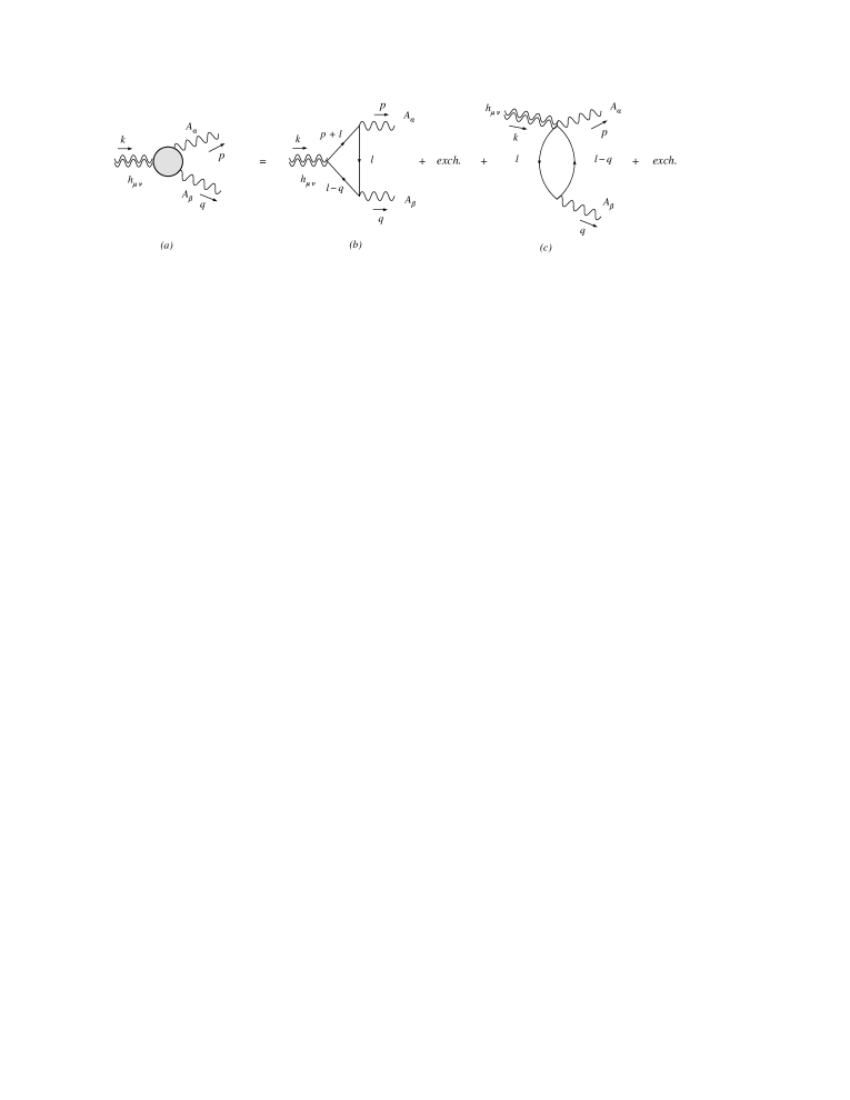
Figure 1: The complete one-loop vertex (a) given by the sum of the 1PI contributions called $V_{55}^{\mu\nu\alpha\beta}(p,q)$ (b) and $W_{55}^{\mu\nu\alpha\beta}(p,q)$ (c) with a graviton $h_{\mu\nu}$ in the initial state and two gauge bosons with axial-vector couplings $A_{\alpha},A_{\beta}$ in the final state.

The relevant diagrams responsible for the conformal anomaly are shown in Fig. 1 and take the form of eqs. (38) and (LABEL:tbubble). They consist of an amplitude with triangular topology (see Fig. 1b) and of a bubble-like diagram (called a “t-bubble”, see Fig. 1c). This has the topology of a self-energy loop inserted on each of the gauge lines and attached from one side to the T vertex. These contributions are all of $O(g^{2})$. At this point, we recall that the tree-level vertex with a graviton and a Dirac fermion, namely $V^{\prime\,\mu\nu}$, and the trilinear graviton-gauge boson-fermion coupling, i.e. $W_{5}^{\prime\,\mu\nu\alpha}$, induced by the two contributions $T_{f}$ and $T_{iA}$ are respectively given by

$$V^{\prime\,\mu\nu}(k_{1},k_{2}) = \frac{1}{4}\left[\gamma^{\mu}(k_{1}+k_{2})^{\nu}+\gamma^{\nu}(k_{1}+k_{2})^{\mu}\right]-\frac{1}{2}g^{\mu\nu}[\gamma^{\lambda}(k_{1}+k_{2})_{\lambda}-2m]$$ (69)

$$W_{5}^{\prime\,\mu\nu\alpha} = -\frac{1}{2}(\gamma^{\mu}\gamma_{5}g^{\nu\alpha}+\gamma^{\nu}\gamma_{5}g^{\mu\alpha})+g^{\mu\nu}\gamma^{\alpha}\gamma_{5}$$ (70)

where $k_{1}$ and $k_{2}$ are generic momenta, incoming and outgoing, respectively. Notice that the first contribution is vector-like, derived from (13) and, naturally, is the same appearing in the previous analysis of the $\langle TJJ\rangle$ correlator in [2]. The second one, $W_{5}^{\prime\,\mu\nu\alpha}$, due to (15), differs from the analogous vertex $W^{\prime\,\mu\nu\alpha}$ appearing in the case of the $\langle TJJ\rangle$ correlator because of the presence of the $\gamma_{5}$ matrix.
If we denote with $k$ the incoming momentum of the graviton and with $p$ and $q$ the two outgoing momenta of the $A$ gauge bosons we obtain

$$(2\,\pi)^{4}\,\delta^{4}(k-p-q)\,V_{55}^{\mu\nu\alpha\beta}(p,q)\equiv\int d^{4}x\,d^{4}y\,d^{4}z\,e^{-ik\cdot z+ip\cdot x+iq\cdot y}\,\langle T_{f}^{\mu\nu}(z)\,J_{A}^{\alpha}(x)\,J_{A}^{\beta}(y)\rangle$$ (71)

$$(2\,\pi)^{4}\,\delta^{4}(k-p-q)\,W_{5\,5}^{\mu\nu\alpha\beta}(p,q)\equiv\int d^{4}x\,d^{4}y\,d^{4}z\,e^{-ik\cdot z+ip\cdot x+iq\cdot y}\,\langle T_{iA}^{\mu\nu}(z)J_{A}^{\alpha}(x)J_{A}^{\beta}(y)\rangle.$$ (72)

Explicitly

$$V_{5\,5}^{\mu\nu\alpha\beta}(p,q)=-ig^{2}\int\frac{d^{4}l}{(2\pi)^{4}}\,\frac{{\rm tr}\left\{V^{\prime\,\mu\nu}(l+p,l-q)(l\!\!\!/-q\!\!\!/+m)\gamma^{\beta}\gamma_{5}\,(l\!\!\!/+m)\,\gamma^{\alpha}\gamma_{5}(l\!\!\!/+p\!\!\!/+m)\right\}}{[l^{2}-m^{2}]\,[(l-q)^{2}-m^{2}]\,[(l+p)^{2}-m^{2}]}\,,$$

(73)

$$W_{5\,5}^{\mu\nu\alpha\beta}(p,q)=-ig^{2}\int\frac{d^{4}l}{(2\pi)^{4}}\,\frac{{\rm tr}\left\{W_{5}^{\prime\,\mu\nu\alpha}\,(l\!\!\!/+m)\,\gamma^{\beta}\gamma_{5}(l\!\!\!/+q\!\!\!/+m)\right\}}{[l^{2}-m^{2}]\,[(l+q)^{2}-m^{2}]},$$ (74)

so that the complete one-loop amplitude (see Fig. 1) is built up by symmetrizing on the external boson lines as

$$\Gamma_{AA}^{\mu\nu\alpha\beta}(p,q)=V_{5\,5}^{\mu\nu\alpha\beta}(p,q)+V_{5\,5}^{\mu\nu\beta\alpha}(q,p)+W_{5\,5}^{\mu\nu\alpha\beta}(p,q)+W_{5\,5}^{\mu\nu\beta\alpha}(q,p).$$ (75)

5 Tensor decomposition and naive manipulations

As we have mentioned, the correlator is completely defined by a set of Ward identities, which amount to renormalization conditions which should be imposed in such a way 1) to respect its Bose symmetry and 2) the conservation of the fundamental currents of the theory. This is the case for all the anomalous correlators, both for chiral and conformal anomalies. At the same time, one needs a good regularization scheme in order to proceed with the actual implementation of these conditions, which could be obviously violated. This may require a (final) finite renormalization of the result in order to force the result to satisfy the original Ward identities. In this respect, various regularization schemes are available for chiral vertices, from a partially [11] to a totally anticommuting $\gamma_{5}$. As we have already mentioned, in the computation of the correlator we have used DRED [10], with loop momenta computed in $D$ spacetime dimensions and traces performed in 4 dimensions, and we have verified all the Ward identities formally derived in this work.

5.1 Vanishing of the $TJ_{V}J_{A}$ correlator

We start our analysis by studying the $TJ_{V}J_{A}$ correlator.

For this reason we just recall that this specific correlation function can be extracted by the generating functional

$$\langle T_{p}^{\mu\nu}(z)\rangle_{V,A} \equiv \int D\psi D\bar{\psi}\,\,T^{\mu\nu}_{p}(z)\,\,e^{i\int d^{4}x(\mathcal{L}_{k}(\psi)+g\,J_{V}\cdot V(x)+g\,J_{A}\cdot A(x))}$$ (76)

$$= \langle T^{\mu\nu}_{p}\,e^{i\int d^{4}x\,g\,(\,J_{V}\cdot V(x)+J_{A}\cdot A(x))}\rangle.$$

Here we have introduced two independent sources $J_{V}$ and $J_{A}$. The corresponding correlators are obtained via functional variations respect to the background fields $V$ and $A$, namely

$$\Gamma_{VA}^{\mu\nu\alpha\beta}(z;x,y)\equiv\frac{\delta^{2}\langle T_{p}^{\mu\nu}(z)\rangle_{V,A}}{\delta V_{\alpha}(x)\delta A_{\beta}(y)}\bigg{|}_{V,A=0}=V_{5}^{\mu\nu\alpha\beta}(z;x,y)+W_{5}^{\mu\nu\alpha\beta}(z;x,y).$$ (77)

whose expressions in momentum space are (for the direct and the exchange contributions)

$$V_{5\,dir}^{\mu\nu\alpha\beta}(p,q)=-(-ig)^{2}i^{3}\int\frac{d^{4}l}{(2\pi)^{4}}\,\frac{{\rm tr}\left\{V^{\prime\,\mu\nu}(l+p,l-q)(l\!\!\!/-q\!\!\!/+m)\gamma^{\beta}\,(l\!\!\!/+m)\,\gamma^{\alpha}\gamma_{5}(l\!\!\!/+p\!\!\!/+m)\right\}}{[l^{2}-m^{2}]\,[(l-q)^{2}-m^{2}]\,[(l+p)^{2}-m^{2}]}\,,$$

(78)

$$V_{5\,ex}^{\mu\nu\alpha\beta}(p,q)=-(-ig)^{2}i^{3}\int\frac{d^{4}l}{(2\pi)^{4}}\,\frac{{\rm tr}\left\{V^{\prime\,\mu\nu}(l-p,l+q)(l\!\!\!/-p\!\!\!/+m)\gamma^{\alpha}\gamma_{5}\,(l\!\!\!/+m)\,\gamma^{\beta}(l\!\!\!/+q\!\!\!/+m)\right\}}{[l^{2}-m^{2}]\,[(l+q)^{2}-m^{2}]\,[(l-p)^{2}-m^{2}]}\,,$$

(79)

$$W_{5\,dir}^{\mu\nu\alpha\beta}(p,q)=-(-ig)^{2}i^{3}\int\frac{d^{4}l}{(2\pi)^{4}}\,\frac{{\rm tr}\left\{W^{\prime\,\mu\nu\alpha}\gamma_{5}(l\!\!\!/+m)\gamma^{\beta}\,(l\!\!\!/+q\!\!\!/+m)\,\right\}}{[l^{2}-m^{2}]\,[(l+q)^{2}-m^{2}]}\,,$$ (80)

$$W_{5\,ex}^{\mu\nu\alpha\beta}(p,q)=-(-ig)^{2}i^{3}\int\frac{d^{4}l}{(2\pi)^{4}}\,\frac{{\rm tr}\left\{W^{\prime\,\mu\nu\beta}(l\!\!\!/+m)\gamma^{\alpha}\gamma_{5}\,(l\!\!\!/+p\!\!\!/+m)\,\right\}}{[l^{2}-m^{2}]\,[(l+p)^{2}-m^{2}]}\,,$$ (81)

and where the vertices $V^{\prime\,\mu\nu}$ and $W^{\prime\,\mu\nu\alpha}$ are defined as

$$V^{\prime\,\mu\nu}(k_{1},k_{2}) = \frac{1}{4}\left[\gamma^{\mu}(k_{1}+k_{2})^{\nu}+\gamma^{\nu}(k_{1}+k_{2})^{\mu}\right]-\frac{1}{2}g^{\mu\nu}[\gamma^{\lambda}(k_{1}+k_{2})_{\lambda}-2m],$$ (82)

$$W^{\prime\,\mu\nu\alpha} = -\frac{1}{2}(\gamma^{\mu}g^{\nu\alpha}+\gamma^{\nu}g^{\mu\alpha})+g^{\mu\nu}\gamma^{\alpha}.$$ (83)

We will use the same trick used for the proof of Furry’s theorem to show the vanishing of this correlator, which is formally divergent and therefore ill-defined. For this reason one needs some external Ward identities in order to resolve its structure. For the $TJ_{V}J_{A}$ vertex the situation is quite peculiar since one can show, using DRED and by allowing momentum shifts, that the three Ward identities are indeed homogeneous

$$k_{\mu}\Gamma_{VA}^{\mu\nu\alpha\beta}=p_{\alpha}\Gamma_{VA}^{\mu\nu\alpha\beta}=q_{\beta}\Gamma_{VA}^{\mu\nu\alpha\beta}=0,$$ (84)

while the properties of symmetry of the correlator are respected. Obviously, this indicates that there is a regularization scheme in which the anomaly of the axial-vector current $J_{A}$ does not appear. A closer inspection shows that this result is caused by a cancellation between the direct and the exchange contribution, since the $\epsilon$-tensor is present in each of the two (direct and exchange) diagrams contributing to the vertex, but not in their sum. Indeed, this clearly seems to indicate that this correlator may be vanishing identically. A second argument, based on charge conjugation invariance brings to identical conclusions.

For this reason, we take the expression of the triangle diagram and insert the identity $C^{-1}\,C=1$ - involving the charge conjugation matrix $C$ between every $\gamma$ matrix - together with the relations

$$C\,\gamma^{\mu}\,C^{-1}=-(\gamma^{\mu})^{T},\qquad\qquad C\,\gamma_{5}\,C^{-1}=\gamma_{5},$$ (85)

so that the trace in eq. (5.1) becomes

$$\mathcal{T} = {\rm tr}\left\{\tilde{V}^{\prime\,\mu\nu}(l+p,l-q)^{T}(l\!\!\!/-q\!\!\!/-m)^{T}(\gamma^{\beta})^{T}\,(l\!\!\!/-m)^{T}\,(\gamma^{\alpha})^{T}\gamma_{5}(l\!\!\!/+p\!\!\!/-m)^{T}\right\}$$ (86)

$$= -{\rm tr}\left\{\tilde{V}^{\prime\,\mu\nu}(l+p,l-q)(l\!\!\!/+p\!\!\!/-m)\gamma^{\alpha}\gamma_{5}\,(l\!\!\!/-m)\,\gamma^{\beta}\,(l\!\!\!/-q\!\!\!/-m)\right\}$$

where $\tilde{V}^{\prime\,\mu\nu}$ differs from $V^{\prime\,\mu\nu}$ only for the sign of the mass term

$$\tilde{V}^{\prime\,\mu\nu}(k_{1},k_{2})=\frac{1}{4}\left[\gamma^{\mu}(k_{1}+k_{2})^{\nu}+\gamma^{\nu}(k_{1}+k_{2})^{\mu}\right]-\frac{1}{2}g^{\mu\nu}[\gamma^{\lambda}(k_{1}+k_{2})_{\lambda}+2m].$$ (87)

Changing the integration variable $l\rightarrow-l$ in eq.(86) we get

$$\mathcal{T}=-{\rm tr}\left\{V^{\prime\,\mu\nu}(l-p,l+q)(l\!\!\!/-p\!\!\!/+m)\gamma^{\alpha}\gamma_{5}\,(l\!\!\!/+m)\,\gamma^{\beta}\,(l\!\!\!/+q\!\!\!/+m)\right\},$$ (88)

while the three denominators in eq.(5.1) change according to

$$\frac{1}{[l^{2}-m^{2}]\,[(l-q)^{2}-m^{2}]\,[(l+p)^{2}-m^{2}]}\rightarrow\frac{1}{[l^{2}-m^{2}]\,[(l+q)^{2}-m^{2}]\,[(l-p)^{2}-m^{2}]}.$$ (89)

Combining eq.(88) and (89) it is easy to recognize that

$$V_{5\,dir}^{\mu\nu\alpha\beta}(p,q)=-V_{5\,ex}^{\mu\nu\alpha\beta}(p,q)$$ (90)

so that the sum of the two triangles vanishes.
The last point to check in order to be sure of the vanishing of the vertex concerns the contributions from the t-bubble diagrams. These have been defined in eq.(80) and (81) and their topology is the one showed in Fig. 1c. These are both separately equal to zero because they consists of a combination of 2-point functions of the form $\Pi^{\alpha\beta}_{VA}(p)$ given by

$$\Pi^{\alpha\beta}_{VA}(p)=-g^{2}\,\int\frac{d^{4}l}{(2\pi)^{4}}\,\frac{{\rm tr}\left\{\gamma^{\alpha}\gamma_{5}\,(l\!\!\!/+m)\gamma^{\beta}\,(l\!\!\!/+p\!\!\!/+m)\,\right\}}{[l^{2}-m^{2}]\,[(l+p)^{2}-m^{2}]}$$ (91)

which are also identically vanishing.

$$\begin{array}[]{|c | c | c |c | c |c |}\hline\cr&&&&&\\[-14.22636pt] \begin{array}[t]{c}p^{\mu}p^{\nu}p^{\alpha}p^{\beta}\\ q^{\mu}q^{\nu}q^{\alpha}q^{\beta}\end{array}&\begin{array}[t]{c}p^{\mu}p^{\nu}p^{\alpha}q^{\beta}\\ p^{\mu}p^{\nu}q^{\alpha}p^{\beta}\\ p^{\mu}q^{\nu}p^{\alpha}p^{\beta}\\ q^{\mu}p^{\nu}p^{\alpha}p^{\beta}\end{array}&\begin{array}[t]{c}p^{\mu}p^{\nu}q^{\alpha}q^{\beta}\\ p^{\mu}q^{\nu}p^{\alpha}q^{\beta}\\ q^{\mu}p^{\nu}p^{\alpha}q^{\beta}\end{array}&\begin{array}[t]{c}p^{\mu}q^{\nu}q^{\alpha}p^{\beta}\\ q^{\mu}p^{\nu}q^{\alpha}p^{\beta}\\ q^{\mu}q^{\nu}p^{\alpha}p^{\beta}\end{array}&\begin{array}[t]{c}p^{\mu}q^{\nu}q^{\alpha}q^{\beta}\\ q^{\mu}p^{\nu}q^{\alpha}q^{\beta}\\ q^{\mu}q^{\nu}p^{\alpha}q^{\beta}\\ q^{\mu}q^{\nu}q^{\alpha}p^{\beta}\end{array}&\begin{array}[t]{c}g^{\mu\nu}g^{\alpha\beta}\\ g^{\alpha\mu}g^{\beta\nu}\\ g^{\alpha\nu}g^{\beta\mu}\end{array}\\[59.75095pt] \hline\cr&&&&&\\[-14.22636pt] \begin{array}[]{c}p^{\mu}p^{\nu}g^{\alpha\beta}\\ p^{\mu}q^{\nu}g^{\alpha\beta}\\ q^{\mu}p^{\nu}g^{\alpha\beta}\\ q^{\mu}q^{\nu}g^{\alpha\beta}\end{array}&\begin{array}[]{c}p^{\beta}p^{\nu}g^{\alpha\mu}\\ p^{\beta}q^{\nu}g^{\alpha\mu}\\ q^{\beta}p^{\nu}g^{\alpha\mu}\\ q^{\beta}q^{\nu}g^{\alpha\mu}\end{array}&\begin{array}[]{c}p^{\beta}p^{\mu}g^{\alpha\nu}\\ p^{\beta}q^{\mu}g^{\alpha\nu}\\ q^{\beta}p^{\mu}g^{\alpha\nu}\\ q^{\beta}q^{\mu}g^{\alpha\nu}\end{array}&\begin{array}[]{c}p^{\alpha}p^{\nu}g^{\beta\mu}\\ p^{\alpha}q^{\nu}g^{\beta\mu}\\ q^{\alpha}p^{\nu}g^{\beta\mu}\\ q^{\alpha}q^{\nu}g^{\beta\mu}\end{array}&\begin{array}[]{c}p^{\mu}p^{\alpha}g^{\beta\nu}\\ p^{\mu}q^{\alpha}g^{\beta\nu}\\ q^{\mu}p^{\alpha}g^{\beta\nu}\\ q^{\mu}q^{\alpha}g^{\beta\nu}\end{array}&\begin{array}[]{c}p^{\alpha}p^{\beta}g^{\mu\nu}\\ p^{\alpha}q^{\beta}g^{\mu\nu}\\ q^{\alpha}p^{\beta}g^{\mu\nu}\\ q^{\alpha}q^{\beta}g^{\mu\nu}\end{array}\\[34.14322pt] \hline\cr\end{array}$$

Table 1: The 43 tensor monomials called $l_{i}^{\mu\nu\alpha\beta}(p,q)$ built up from the metric tensor and the two independent momenta $p$ and $q$ into which a general fourth rank tensor can be expanded.

5.2 The computation of the $\langle TJ_{A}J_{A}\rangle$ correlator

We now going to address the computation of the $TJ_{A}J_{A}$ vertex, but prior to that we briefly review the vector/vector case. As discussed in [1] and in [2] the full one-loop amplitude with the energy momentum tensor coupled to two vector currents, $\Gamma^{\mu\nu\alpha\beta}_{VV}$, can be expanded on the basis provided by the 43 monomial tensors $l_{i}^{\mu\nu\alpha\beta}(p,q)$ listed in Tab. 1

$$\Gamma_{VV}^{\mu\nu\alpha\beta}(p,q)=\,\sum_{i=1}^{43}\,A_{i}(k^{2},p^{2},q^{2})\,l_{i}^{\mu\nu\alpha\beta}(p,q),$$ (92)

whose form factors $A_{i}(k^{2},p^{2},q^{2})$ are not all convergent, since the amplitude has total mass dimension equal to $2$. It has been shown in [2] that they can be divided into $3$ groups:

• $A_{1}\leq A_{i}\leq A_{16}$ - multiplied by a product of four momenta, they have mass dimension $-2$ and therefore are UV finite;

• $A_{17}\leq A_{i}\leq A_{19}$ - these have mass dimension $2$ since the four Lorentz indices of the amplitude are carried by two metric tensors

• $A_{20}\leq A_{i}\leq A_{43}$ - they appear next to a metric tensor and two momenta, have mass dimension $0$ and are divergent.

In [1] the $43$ invariant amplitudes $A_{i}(k^{2},p^{2},q^{2})$ have been cleverly reduced to the $13$ named $F_{i}(k^{2},p^{2},q^{2})$. A similar result is obtained in [2] using a different intermediate basis. This reorganization of the amplitude shows conclusively that the effective action of theories with conformal anomalies is affected by anomaly poles which contain the entire signature of the anomaly [12].

As we are going to show, a similar result holds also for the $\langle TJ_{A}J_{A}\rangle$ vertex. At the same time, we are going to demonstrate the appearance only of conformal anomalies, since the mixed anomalies cancel, and present the complete expression of this vertex.

$$\begin{array}[]{|c|c|}\hline\cr i&t_{i}^{\mu\nu\alpha\beta}(p,q)\\ \hline\cr\hline\cr 1&\left(k^{2}g^{\mu\nu}-k^{\mu}k^{\nu}\right)u^{\alpha\beta}(p.q)\\ \hline\cr 2&\left(k^{2}g^{\mu\nu}-k^{\mu}k^{\nu}\right)w^{\alpha\beta}(p.q)\\ \hline\cr 3&\left(p^{2}g^{\mu\nu}-4p^{\mu}p^{\nu}\right)u^{\alpha\beta}(p.q)\\ \hline\cr 4&\left(p^{2}g^{\mu\nu}-4p^{\mu}p^{\nu}\right)w^{\alpha\beta}(p.q)\\ \hline\cr 5&\left(q^{2}g^{\mu\nu}-4q^{\mu}q^{\nu}\right)u^{\alpha\beta}(p.q)\\ \hline\cr 6&\left(q^{2}g^{\mu\nu}-4q^{\mu}q^{\nu}\right)w^{\alpha\beta}(p.q)\\ \hline\cr 7&\left[p\cdot q\,g^{\mu\nu}-2(q^{\mu}p^{\nu}+p^{\mu}q^{\nu})\right]u^{\alpha\beta}(p.q)\\ \hline\cr 8&\left[p\cdot q\,g^{\mu\nu}-2(q^{\mu}p^{\nu}+p^{\mu}q^{\nu})\right]w^{\alpha\beta}(p.q)\\ \hline\cr 9&\left(p\cdot q\,p^{\alpha}-p^{2}q^{\alpha}\right)\big{[}p^{\beta}\left(q^{\mu}p^{\nu}+p^{\mu}q^{\nu}\right)-p\cdot q\,(g^{\beta\nu}p^{\mu}+g^{\beta\mu}p^{\nu})\big{]}\\ \hline\cr 10&\big{(}p\cdot q\,q^{\beta}-q^{2}p^{\beta}\big{)}\,\big{[}q^{\alpha}\left(q^{\mu}p^{\nu}+p^{\mu}q^{\nu}\right)-p\cdot q\,(g^{\alpha\nu}q^{\mu}+g^{\alpha\mu}q^{\nu})\big{]}\\ \hline\cr 11&\left(p\cdot q\,p^{\alpha}-p^{2}q^{\alpha}\right)\big{[}2\,q^{\beta}q^{\mu}q^{\nu}-q^{2}(g^{\beta\nu}q^{\mu}+g^{\beta\mu}q^{\nu})\big{]}\\ \hline\cr 12&\big{(}p\cdot q\,q^{\beta}-q^{2}p^{\beta}\big{)}\,\big{[}2\,p^{\alpha}p^{\mu}p^{\nu}-p^{2}(g^{\alpha\nu}p^{\mu}+g^{\alpha\mu}p^{\nu})\big{]}\\ \hline\cr 13&\big{(}p^{\mu}q^{\nu}+p^{\nu}q^{\mu}\big{)}g^{\alpha\beta}+p\cdot q\,\big{(}g^{\alpha\nu}g^{\beta\mu}+g^{\alpha\mu}g^{\beta\nu}\big{)}-g^{\mu\nu}u^{\alpha\beta}\\ &-\big{(}g^{\beta\nu}p^{\mu}+g^{\beta\mu}p^{\nu}\big{)}q^{\alpha}-\big{(}g^{\alpha\nu}q^{\mu}+g^{\alpha\mu}q^{\nu}\big{)}p^{\beta}\\ \hline\cr\end{array}$$

Table 2: The 13 fourth rank tensors $t_{i}^{\mu\nu\alpha\beta}(p,q)$ satisfying the vector current conservation on the external lines with momenta $p$ and $q$.

To illustrate this point, we observe that the insertion of the non-chiral component of $T^{\mu\nu}$ (represented by $T_{f}^{\mu\nu}$) in the correlator $V_{55}$, defines one of the two subamplitudes which may potentially generate mixed anomalies. On the other hand, it is however obvious - by a glance at the structure of the correlator - that we could remove symmetrically the chiral matrix all together. Therefore, the $\langle TJ_{A}J_{A}\rangle$ correlator can be split in two terms, the first being the correlator with two vector currents called $TJ_{V}J_{V}$, while the second is an extra contribution, proportional to the fermion mass $m$, denoted by $\Omega$

$$\Gamma_{AA}^{\mu\nu\alpha\beta}(p,q)=\Gamma_{VV}^{\mu\nu\alpha\beta}(p,q)+\Omega^{\mu\nu\alpha\beta}(p,q).$$ (93)

The explicit computation of the correlator with two vector currents $\Gamma_{VV}^{\mu\nu\alpha\beta}$ can be borrowed from [2], but the computation of the extra terms is very involved, due to the need to select a specific number of tensor structures in its expansion. Notice that the decomposition in eq. (93) is particularly useful because shows that the vector and axial-vector cases coincide in the chiral limit, i.e. for $\Omega^{\mu\nu\alpha\beta}=0$.
As we have just mentioned above, the amplitude $\Gamma^{\mu\nu\alpha\beta}_{VV}$ can be expanded in the reduced basis given in Tab. 2

$$\Gamma_{VV}^{\mu\nu\alpha\beta}(p,q)=\,\sum_{i=1}^{13}F_{i}(s;s_{1},s_{2},m^{2})\ t_{i}^{\mu\nu\alpha\beta}(p,q)\,,$$ (94)

where the invariant amplitudes $F_{i}(s;s_{1},s_{2},m^{2})$ are functions of the kinematical invariants $s=k^{2}=(p+q)^{2}$, $s_{1}=p^{2}$, $s_{2}=q^{2}$. Their explicit expressions in the general case have been given in [2]. In the simplest case, i.e. for an internal zero mass fermion ($m=0$) and on-shell photons on the external lines ($s_{1}=s_{2}=0$), the only non-vanishing $F_{i}(s;s_{1},s_{2},m^{2})$ are given by

$$F_{1}(s,0,0,0) = -\frac{g^{2}}{18\pi^{2}s},$$ (95)

$$F_{3}(s,0,0,0) = F_{5}(s,0,0,0)=-\frac{g^{2}}{144\pi^{2}\,s},$$ (96)

$$F_{7}(s,0,0,0) = -4\,F_{3}(s,0,0,0),$$ (97)

$$F_{13,R}(s,0,0,0) = -\frac{g^{2}}{144\pi^{2}}\,\left[12\log\left(-\frac{s}{\mu^{2}}\right)-35\right],$$ (98)

(with $s<0$) where $F_{13}$ is affected by charge renormalization (with a scale $\mu$). As we are going to discuss next, $F_{1}$ is the only form factor contributing to the trace anomaly in the massless case, and contains an anomaly pole. In this sense we can say that the pole saturates the anomaly and completely accounts for it. In [1] this $1/s$ terms is identified by a spectral analysis of the correlator, while the same structure emerges form the complete expressions of the form factors derived in [2] and presented above.

Coming instead to the new contribution $\Omega^{\mu\nu\alpha\beta}$ appearing in eq. (93), this can be written as

$$\Omega^{\mu\nu\alpha\beta}(p,q)=\Omega_{V}^{\mu\nu\alpha\beta}(p,q)+\Omega_{V}^{\mu\nu\beta\alpha}(q,p)+\Omega_{W}^{\mu\nu\alpha\beta}(p,q)+\Omega_{W}^{\mu\nu\beta\alpha}(q,p),$$ (99)

where the amplitudes $\Omega_{V}^{\mu\nu\alpha\beta}$ and $\Omega_{W}^{\mu\nu\alpha\beta}$ are given by

$$\Omega_{V}^{\mu\nu\alpha\beta}(p,q)=-2m(-ig^{2})\int\frac{d^{4}l}{(2\pi)^{4}}\,\frac{{\rm tr}\left\{V^{\prime\,\mu\nu}(l+p,l-q)(l\!\!\!/-q\!\!\!/+m)\gamma^{\beta}\gamma^{\alpha}(l\!\!\!/+p\!\!\!/+m)\right\}}{[l^{2}-m^{2}]\,[(l-q)^{2}-m^{2}]\,[(l+p)^{2}-m^{2}]}\,,$$

(100)

$$\Omega_{W}^{\mu\nu\alpha\beta}(p,q)=-2m(-ig^{2})\int\frac{d^{4}l}{(2\pi)^{4}}\,\frac{{\rm tr}\left\{W^{\prime\,\mu\nu\alpha}\,\gamma^{\beta}(l\!\!\!/+q\!\!\!/+m)\right\}}{[l^{2}-m^{2}]\,[(l+q)^{2}-m^{2}]},$$ (101)

with the $V^{\prime\,\mu\nu}$ and $W^{\prime\,\mu\nu\alpha}$ defined in eqs (82) and (83). The remaining two terms in eq. (99) are simply the Bose symmetric amplitudes obtained exchanging the indices $\alpha$ and $\beta$ and the momenta $p$ and $q$ of (5.2) and (101). The extra term $\Omega^{\mu\nu\alpha\beta}$ can be expanded on the basis provided by the 43 monomial tensors $l_{i}^{\mu\nu\alpha\beta}(p,q)$ listed in Tab. 1

$$\Omega^{\mu\nu\alpha\beta}(p,q)=\,\sum_{i=1}^{43}\,E_{i}(k^{2},p^{2},q^{2},m^{2})\,l_{i}^{\mu\nu\alpha\beta}(p,q),$$ (102)

where the form factors $E_{i}(k^{2},p^{2},q^{2},m^{2})$ are some functions of the kinematical variables and of the mass of the fermion in the loop. This needs to be identified by a direct inspection. The explicit computation shows that not all the 43 invariant amplitudes $E_{i}(k^{2},p^{2},q^{2},m^{2})$ are really present in this expansion and therefore the surviving ones can be appropriately combined in a lower number of composite tensor structures. This result can be organized in a more compact form after introducing a new tensor basis whose elements $f_{i}^{\mu\nu\alpha\beta}(p,q)$ ($i=1,\dots,9$) are listed in Tab.3. We obtain

$$\Omega^{\mu\nu\alpha\beta}(p,q)=\,\sum_{i=1}^{9}\,R_{i}(s,s_{1},s_{2},m^{2})\,f_{i}^{\mu\nu\alpha\beta}(p,q),$$ (103)

where the invariant amplitudes $R_{i}(s,s_{1},s_{2},m^{2})$ depend on the kinematical variables $s=k^{2}=(p+q)^{2}$, $s_{1}=p^{2}$, $s_{2}=q^{2}$ besides the fermion mass $m$.
Three of the nine tensors are Bose symmetric, namely,

$$f_{i}^{\mu\nu\alpha\beta}(p,q)=f_{i}^{\mu\nu\beta\alpha}(q,p)\,,\qquad i=1,6,9\,,$$ (104)

while the remaining ones form three pairs related by Bose symmetry

$$f_{2}^{\mu\nu\alpha\beta}(p,q)=f_{3}^{\mu\nu\beta\alpha}(q,p)\,,$$ (105)

$$f_{4}^{\mu\nu\alpha\beta}(p,q)=f_{5}^{\mu\nu\beta\alpha}(q,p)\,,$$ (106)

$$f_{7}^{\mu\nu\alpha\beta}(p,q)=f_{8}^{\mu\nu\beta\alpha}(q,p)\,.$$ (107)

This basis is particularly useful because only the first three of the nine tensors have a non-zero trace

$$g_{\mu\nu}f_{1}^{\mu\nu\alpha\beta}(p,q) = 3k^{2}g^{\alpha\beta}\,,$$ (108)

$$g_{\mu\nu}f_{2}^{\mu\nu\alpha\beta}(p,q) = g_{\mu\nu}f_{3}^{\mu\nu\alpha\beta}(p,q)=2(p^{\alpha}q^{\beta}-p^{\beta}q^{\alpha})\,,$$ (109)

while the remaining six tensors are traceless

$$g_{\mu\nu}f_{i}^{\mu\nu\alpha\beta}(p,q)=0\,,\qquad i=4,5,6,7,8,9\,.$$ (110)

At this point, the goal is to express the amplitude $\Omega^{\mu\nu\alpha\beta}(p,q)$ in an analytical form. We start from the evaluation of the integrals in eqs. (5.2) and (101), obtaining the form factors $E_{i}$. At a second stage we map them into the new parameterization defined in eq. (103), determining in this way the coefficients $R_{i}$. The relations between the two sets $\{E_{i}\}_{i=1,\dots,43}$ and $\{R_{i}\}_{i=1,\dots,9}$, for the most general external momenta are

$$R_{1} = \frac{1}{3k^{2}}\left(E_{20}\,p^{2}+2E_{21}\,p\cdot q+E_{23}\,q^{2}+4E_{17}+2E_{18}\right),$$ (111)

$$R_{2} = E_{26},$$ (112)

$$R_{3} = E_{33},$$ (113)

$$R_{4} = E_{26},$$ (114)

$$R_{5} = E_{33},$$ (115)

$$R_{6} = \frac{E_{18}}{p\cdot q},$$ (116)

$$R_{7} = -\frac{1}{12k^{2}}\left(E_{20}\,p^{2}+2E_{21}\,p\cdot q+E_{23}\,q^{2}+4E_{17}+2E_{18}\right)-\frac{E_{20}}{4},$$ (117)

$$R_{8} = -\frac{1}{12k^{2}}\left(E_{20}\,p^{2}+2E_{21}\,p\cdot q+E_{23}\,q^{2}+4E_{17}+2E_{18}\right)-\frac{E_{23}}{4},$$ (118)

$$R_{9} = -\frac{1}{6k^{2}}\left(E_{20}\,p^{2}+2E_{21}\,p\cdot q+E_{23}\,q^{2}+4E_{17}+2E_{18}\right)+\frac{E_{18}}{2p\cdot q}-\frac{E_{21}}{2},$$ (119)

$$\begin{array}[]{|c|c|}\hline\cr i&f_{i}^{\mu\nu\alpha\beta}(p,q)\\ \hline\cr\hline\cr 1&\left(k^{2}g^{\mu\nu}-k^{\mu}k^{\nu}\right)g^{\alpha\beta}\\ \hline\cr 2&p^{\nu}q^{\beta}g^{\alpha\mu}+p^{\mu}q^{\beta}g^{\alpha\nu}-p^{\nu}q^{\alpha}g^{\beta\mu}-p^{\mu}q^{\alpha}g^{\beta\nu}\\ \hline\cr 3&p^{\alpha}q^{\nu}g^{\beta\mu}+p^{\alpha}q^{\mu}g^{\beta\nu}-p^{\beta}q^{\nu}g^{\alpha\mu}-p^{\beta}q^{\mu}g^{\alpha\nu}\\ \hline\cr 4&p^{\nu}p^{\beta}g^{\alpha\mu}+p^{\mu}p^{\beta}g^{\alpha\nu}-p^{\nu}p^{\alpha}g^{\beta\mu}-p^{\mu}p^{\alpha}g^{\beta\nu}\\ \hline\cr 5&q^{\alpha}q^{\nu}g^{\beta\mu}+q^{\alpha}q^{\mu}g^{\beta\nu}-q^{\beta}q^{\nu}g^{\alpha\mu}-q^{\beta}q^{\mu}g^{\alpha\nu}\\ \hline\cr 6&(p^{\mu}q^{\nu}+q^{\mu}p^{\nu})g^{\alpha\beta}+p\cdot q\,(g^{\alpha\nu}g^{\beta\mu}+g^{\alpha\mu}g^{\beta\nu}-g^{\alpha\beta}g^{\mu\nu})\\ \hline\cr 7&\left(p^{2}g^{\mu\nu}-4p^{\mu}p^{\nu}\right)g^{\alpha\beta}\\ \hline\cr 8&\left(q^{2}g^{\mu\nu}-4q^{\mu}q^{\nu}\right)g^{\alpha\beta}\\ \hline\cr 9&\left(p\cdot qg^{\mu\nu}-2(q^{\mu}p^{\nu}+p^{\mu}q^{\nu})\right)g^{\alpha\beta}\\ \hline\cr\end{array}$$

Table 3: Basis of 9 fourth rank tensors called $f_{i}^{\mu\nu\alpha\beta}(p,q)$.

where all the dependence on the kinematical invariants $k^{2},p^{2},q^{2}$ and $m^{2}$ appearing in the sets $R_{i}$ and $E_{i}$ has been omitted. The explicit expressions in DRED of the form factors $R_{i}$ have been collected in Appendix B and represent an important step in the computation of the $\langle TJ_{A}J_{A}\rangle$ correlator. These form factors are affected by the usual ultraviolet singularities, which in a renormalizable theory would be removed by standard renormalization counterterms. In our case they turn out to be proportional to 2-point functions.

Except for these possible counterterms, the main techniques and methods used in this analysis remain invariant and are of an easy application also in the case of the Standard Model. Notice, in particular, that the main equation (93) implies that the non-renormalizable contributions are proportional to mass corrections contributing to $\Omega$, and the non-renormalizable terms indeed involve correlators of two axial-vector currents, as just mentioned above. The renormalization of the first contribution $\Gamma_{VV}$ is canonical, and is attributed to the form factor $F_{13}$ of Eq. (98), which is induced by a renormalization of 2-point functions of vector currents.

Figure 2: Chiral decomposition of the correlator.

Before coming to the analysis of the other vertices, in closing this section we just remark that our analysis in the V/A basis can be rewritten completely in terms of chiral L/R currents, since the following relations hold for nonzero $m$

$$\langle TJ_{V}J_{V}\rangle = \langle TJ_{L}J_{L}\rangle+\langle TJ_{R}J_{R}\rangle+\langle TJ_{L}J_{R}\rangle+\langle TJ_{R}J_{L}\rangle,$$ (120)

$$\langle TJ_{A}J_{A}\rangle = \langle TJ_{L}J_{L}\rangle+\langle TJ_{R}J_{R}\rangle-\langle TJ_{L}J_{R}\rangle-\langle TJ_{R}J_{L}\rangle,$$ (121)

$$\langle TJ_{A}J_{A}\rangle=\langle TJ_{V}J_{V}\rangle-2\left(\langle TJ_{L}J_{R}\rangle+\langle TJ_{R}J_{L}\rangle\right).$$ (122)

$$\langle TJ_{L}J_{L}\rangle=\langle TJ_{R}J_{R}\rangle=\frac{1}{4}\left(\langle TJJ\rangle+\langle TJ_{A}J_{A}\rangle\right),$$ (123)

while

$$\langle T_{L}J_{L}J_{L}\rangle=\langle T_{R}J_{R}J_{R}\rangle=\frac{1}{2}\langle TJJ\rangle$$ (124)

is valid for a vanishing fermion mass $m$. The formulation in terms of L/R currents is the most convenient for the study of vertices containing trace anomalies, in the case of realistic theories such as the Standard Model.

6 Trace anomaly of the $\langle TJ_{A}J_{A}\rangle$ correlator

We now move to analyze the trace of the $\langle TJ_{A}J_{A}\rangle$ correlator. We consider generic virtualities of the external lines and a massive fermion.

In the absence of anomalies, the naive trace of the $\Gamma_{AA}^{\mu\nu\alpha\beta}$ amplitude is simply obtained by replacing the partial energy-momentum tensor $T_{p}^{\mu\nu}$ in the $\langle TJ_{A}J_{A}\rangle$ correlator with its classical trace $T_{p\,\mu}^{\mu}=-m\bar{\psi}\psi$ and it is given by

$$\Lambda_{AA}^{\alpha\beta}(p,q) = -m\,(ig)^{2}\int d^{4}x\,d^{4}y\,e^{ip\cdot x+iq\cdot y}\langle\bar{\psi}\psi J_{A}^{\alpha}(x)J_{A}^{\beta}(y)\rangle$$ (125)

$$= -m\,g^{2}\,\int\frac{d^{4}l}{(2\pi)^{4}}\,tr\left\{\frac{i}{l\!\!\!/-q\!\!\!/-m}\gamma^{\beta}\gamma_{5}\frac{i}{l\!\!\!/-m}\gamma^{\alpha}\gamma_{5}\frac{i}{l\!\!\!/+p\!\!\!/-m}\right\}+\textrm{exch.}$$

As in eq. (93) we can split the $\Lambda_{A\,A}^{\alpha\beta}$ into two terms: the first, $\Lambda_{VV}^{\alpha\beta}$, being the classical trace obtained from the $\langle TJ_{V}J_{V}\rangle$ correlator, whereas the second, $\Lambda_{\Omega}^{\alpha\beta}$, takes into account the axial contribution to the amplitude as

$$\Lambda_{AA}^{\alpha\beta}(p,q)=\Lambda_{VV}^{\alpha\beta}(p,q)+\Lambda_{\Omega}^{\alpha\beta}(p,q).$$ (126)

The $\Lambda^{\alpha\beta}_{VV}$ amplitude refers to the $\langle TJ_{V}J_{V}\rangle$ correlator. It can be written in the form

$$\Lambda_{VV}^{\alpha\beta}(p,q)=G_{1}(s,s_{1},s_{2},m^{2})\,u^{\alpha\beta}(p,q)+G_{2}(s,s_{1},s_{2},m^{2})\,w^{\alpha\beta}(p,q),$$ (127)

where the rank-2 tensors are defined by

$$u^{\alpha\beta}(p,q)\equiv(p\cdot q)\,g^{\alpha\beta}-q^{\alpha}\,p^{\beta}\,,$$ (128)

$$w^{\alpha\beta}(p,q)\equiv p^{2}\,q^{2}\,g^{\alpha\beta}+(p\cdot q)\,p^{\alpha}\,q^{\beta}-q^{2}\,p^{\alpha}\,p^{\beta}-p^{2}\,q^{\alpha}\,q^{\beta},$$ (129)

with coefficients $G_{i}(s,s_{1},s_{2},m^{2})$ which are left to an Appendix (Appendix C).
The second term $\Lambda_{\Omega}^{\alpha\beta}$ in eq.(126) can be decomposed into two tensorial structures as

$$\Lambda_{\Omega}^{\alpha\beta}(p,q)=H_{1}(s,s_{1},s_{2},m^{2})g^{\alpha\beta}+H_{2}(s,s_{1},s_{2},m^{2})(p^{\alpha}q^{\beta}-q^{\alpha}p^{\beta})$$ (130)

where the functions $H_{i}$ are related to the invariant amplitudes $R_{i}$ listed in Appendix B by the relations

$$3sR_{1}(s,s_{1},s_{2},m^{2})=H_{1}(s,s_{1},s_{2},m^{2})-\frac{g^{2}m^{2}}{\pi^{2}}\,,$$ (131)

$$2R_{2}(s,s_{1},s_{2},m^{2})+2R_{3}(s,s_{1},s_{2},m^{2})=H_{2}(s,s_{1},s_{2},m^{2})\,.$$ (132)

The analytical expressions of the off-shell $H_{i}(s,s_{1},s_{2},m^{2})$ form factors are given by

$$H_{1}(s,s_{1},s_{2},m^{2}) = \frac{g^{2}\,m^{2}}{2\pi^{2}}\bigg{[}\mathcal{D}_{1}(s,s_{1},m^{2})+\mathcal{D}_{2}(s,s_{2},m^{2})-2\mathcal{B}_{0}(s^{2},m^{2})+(s-4m^{2})\mathcal{C}_{0}(s,s_{1},s_{2},m^{2})\bigg{]},$$

$$H_{2}(s,s_{1},s_{2},m^{2}) = \frac{g^{2}m^{2}}{\pi^{2}\sigma}\bigg{[}(s+s_{1}-s_{2})\mathcal{D}_{1}(s,s_{1},m^{2})+(s-s_{1}+s_{2})\mathcal{D}_{2}(s,s_{2},m^{2})$$ (133)

$$+ s(s-s_{1}-s_{2})\mathcal{C}_{0}(s,s_{1},s_{2},m^{2})\bigg{]},$$

where $\sigma\equiv s^{2}-2(s_{1}+s_{2})\,s+(s_{1}-s_{2})^{2}$ and the scalar integrals $\mathcal{B}_{0}(s^{2},m^{2})$, $\mathcal{D}_{1}(s,s_{1},m^{2})$, $\mathcal{D}_{2}(s,s_{1},m^{2})$, $\mathcal{C}_{0}(s,s_{1},s_{2},m^{2})$ for generic virtualities and masses are defined in Appendix A.

Tracing the $\Gamma_{AA}^{\mu\nu\alpha\beta}$ correlator we obtain the relation

$$g_{\mu\nu}\Gamma_{AA}^{\mu\nu\alpha\beta}(p,q)=\Lambda_{AA}^{\alpha\beta}(p,q)-\frac{g^{2}}{6\pi^{2}}u^{\alpha\beta}(p,q)-\frac{g^{2}m^{2}}{\pi^{2}}g^{\alpha\beta},$$ (134)

where the first term on the right-hand-sice is the trace anomaly appearing already in the $\langle TJ_{V}J_{V}\rangle$ correlator. The second term, proportional to $m^{2}$, comes from the axial extra term $\Omega^{\mu\nu\alpha\beta}$ and denotes an additional explicit breaking related to the fermion mass. In particular, the anomaly $-\frac{g^{2}}{6\pi^{2}}u^{\alpha\beta}$ is carried by the form factor $F_{1}$, whose expression is given in [2], whereas the mass correction $-{g^{2}m^{2}}/{\pi^{2}}g^{\alpha\beta}$ is induced by $R_{1}$. This additional contribution is gauge variant and its origin can be traced back to the breaking of the $U(1)_{A}$ gauge symmetry due to the fermion mass term.
In the conformal limit the anomalous trace equation (134) takes a simpler form because, as we have already discussed in the previous sections, the $\langle TJ_{A}J_{A}\rangle$ correlator reduces to the $\langle TJ_{V}J_{V}\rangle$ and we obtain

Figure 3: Polar form of the correlator for external on-shell lines: (a) the contribution to the spectral density from the collinear on-shell region of the anomaly loop; (b) the pole as virtual exchange in $\Gamma^{anom}$.

$$g_{\mu\nu}\Gamma_{AA}^{\mu\nu\alpha\beta}(p,q)\bigg{|}_{m=0}=g_{\mu\nu}\Gamma_{VV}^{\mu\nu\alpha\beta}(p,q)\bigg{|}_{m=0}=-\frac{g^{2}}{6\pi^{2}}u^{\alpha\beta}(p,q).$$ (135)

We give in Appendix B the general expression of the form factors $R_{i}$ ($i=1,\dots,9$), which, combined with the results of the 13 form factors $F_{j}$, characterize completely the contributions to the effective action of a vector/axial-vector abelian theory mediated by the conformal anomaly.

Concerning the connection between the anomalous contribution and the $\beta$ function of the theory, also in this case remain valid our previous conclusions, given in [1, 2]. Specifically, we just recall, at this point, that in the (mass independent) regularization scheme $\overline{MS}$ scheme, the $e^{2}$ term in the trace is directly related to the $\beta$ function in this scheme since $\beta(g)={g^{3}}/{(12\pi^{2})}$. In particular, the form factor $F_{13}$ is affected by renormalization via the electric charge [1] [2].

We close this section with few remarks concerning the structure of the effective action for these types of theories, which can be identified from the variational integration of the anomaly equation [13]. This approach is, in a way, complementary to the strategy that we follow, based on a direct computation. As shown in [1] there is perfect agreement between the operatorial structure of variational solution, which also exhibits a $1/\square$ effective interaction, and the anomaly pole found in our analysis. In the variational solution of [13], the $1/s$ massless exchange appears after a linearization of the same solution around the flat spacetime limit, as pointed out in [1]. In fact, one obtains in the weak gravitational field limit

$$S_{anom}[g,A]=-\frac{c}{6}\int d^{4}x\sqrt{-g}\int d^{4}x^{\prime}\sqrt{-g^{\prime}}\,R^{(1)}_{x}\,\square^{-1}_{x,x^{\prime}}\,[F_{\alpha\beta}F^{\alpha\beta}]_{x^{\prime}}\,,$$ (136)

$(c=-g^{2}/(24\pi^{2}))$. In this case

$$R^{(1)}_{x}\equiv\partial^{x}_{\mu}\,\partial^{x}_{\nu}\,h^{\mu\nu}-\square\,h,\qquad h=\eta_{\mu\nu}\,h^{\mu\nu}$$ (137)

is the linearized scalar curvature. As in the case of the TJJ correlator [1] the anomalous contribution to the trace is all contained in the (conformal) anomaly pole (Fig. 3 b)

$$\Gamma_{anom}^{\mu\nu\alpha\beta}(p,q)=\int\,d^{4}x\,\int\,d^{4}y\,e^{ip\cdot x+iq\cdot y}\,\frac{\delta^{2}T^{\mu\nu}_{anom}(0)}{\delta A_{\alpha}(x)\delta A_{\beta}(y)}=\frac{g^{2}}{18\pi^{2}}\frac{1}{k^{2}}\left(g^{\mu\nu}k^{2}-k^{\mu}k^{\nu}\right)u^{\alpha\beta}(p,q)\,,$$ (138)

where [1]

$$T^{\mu\nu}_{anom}(z)=\frac{c}{3}\left(g^{\mu\nu}\square-\partial^{\mu}\partial^{\nu}\right)_{z}\int\,d^{4}x^{\prime}\,\square_{z,x^{\prime}}^{-1}\left[F_{\alpha\beta}F^{\alpha\beta}\right]_{x^{\prime}}.$$ (139)

This effective action is trivially obtained from the tensor structure $F_{1}t_{1}^{\mu\nu\alpha\beta}$, present in the expansion of $\Gamma^{\mu\nu\alpha\beta}$ and accounts for the full trace of the correlator in the massless fermion limit, as shown in Eq. (135).

6.1 Infrared couplings of the anomaly poles and UV behaviour

Before coming to conclusions, we pause here in order to comment on these results and on their meaning on a wider perspective.

We recall that a similar analysis in the QED case [1, 2] also manifests such pole singularities, which appear to be rather generic in anomaly amplitudes. They can be attributed, diagrammatically, to specific configurations of the loop momenta, as illustrated in Fig. (3). The diagram in this figure describes a massive external line decaying into two massless intermediate fermions, in turn decaying into two on-shell axial (or vector) lines (the equivalence between the axial and the vector case in the massless limit is the content of Eq. 93 ($\Omega\to 0$)).

The pole is detected by a computation of the spectral density ($\rho(s)$), which turns out to be proportional to a delta-function $(\rho(s)\sim\delta(s))$. $\rho(s)$ can be found just by evaluating the $s$-channel cut of the anomalous graph using Cutkovsky rules. This approach, as discussed before [1, 2], allows to identify the anomaly poles which are of infrared origin ($s\sim 0$). Other contributions, also characterized by form factors of the form $1/s$, as we have shown, appear in the anomalous amplitude when one performs an off-shell computation of the anomalous correlator. These contributions describe the UV behaviour of an anomalous amplitude ($s\to\infty$) and as such they are usually referred to as “ultraviolet poles”, although the name is slightly misleading, being only generated after an asymptotic expansion of the massive correlator. In fact, the residue of the correlator as $s\to 0$ is indeed vanishing in the massive fermion case [2], showing that no pole is coupled in this limit. Apart from this important detail, it is however correct to retain their appearance in a perturbative computation - even in the UV region - as a manifestation of the same phenomenon of the trace anomaly. In the case of the chiral anomaly the situation is identical.

These computations [2] show that the asymptotic expansion - at large energy - of the regulated graphs responsible for the trace anomaly can be accompanied by corrections which are suppressed as $m^{2}/s^{2}$ (as $s\gg m^{2}$) in the high energy limit, where $m$ is the mass of the fermion in the virtual loop. This organization of the effective action in the UV region allows to recover the ordinary radiative breaking of scale invariance at high energy, being mass corrections negligible in this regime. The use of a mass-independent regularization scheme, such as DRED or DR, is perfectly well taylored in this case, since the separation between pole term and mass corrections involves an asymptotic expansion (at high energy). In particular the $\beta$ function computed in such schemes consistently accounts for the UV running of the coupling [2].

We have described this point at length in the case of the gauge anomaly in [14], to which we refer for more details. This implies that the anomaly is saturated by a pole in very different kinematical regions, in agreement with previous analysis performed in chiral theories [14, 15].

These conclusions show that the description of the effective action in terms of two auxiliary fields - which are introduced in order to recover the local form of the Lagrangian - is significant both in massless theories [1, 16] (for instance on null surfaces, i.e. $s=0$), but also in the high energy domain, for large values of $s$. We refer to [1, 16] for a discussion of the auxiliary field formulation. Similar arguments have been presented in [8, 14, 17] for the axion pole in the chiral coupling of anomalous $U(1)$’s (in the $AVV$ vertex), proving that these auxiliary degrees of freedom are the most significant signature of chiral and conformal anomalies.

7 Conclusions

We have presented an off-shell computation of the correlator of the energy momentum tensor and two vector/axial-vector currents in a chiral theory with an anomalous fermion spectrum, useful for the study of the coupling of anomalous $U(1)$’s to gravity. These interactions are mediated by the trace anomaly. Starting directly from the functional integral, we have derived the Ward identities for the corresponding vertices. These apply, in general, to any correlator of similar type. All the computations have been performed using DRED, and we have shown the cancellation of mixed chiral/conformal anomalies for these types of vertices.

Our computation can be viewed as the generalization of the classical analysis of the $AVV$ diagram to these new vertices. We have allowed explicit mass breaking terms to investigate the most general form of the Ward identities for these correlators, that we anticipate of being of crucial importance for the more general analysis in the Standard Model case.

Obviously, the inclusion of our current study into a theory with spontaneous symmetry breaking and Yukawa couplings, such as the Standard Model, would allow to relate the explicit chiral symmetry breaking terms (mass terms) to the extra interactions of the theory, in particular to the Higgs sector.

We have also shown that, similarly to the case of a vector-like theory, also in the case of a mixed vector/axial-vector theory, the effective action obtained by coupling gravity to the gauge currents is characterized by effective massless degrees of freedom. A more general analysis of these issues and, in particular, an application of the methods developed in this work in the analysis of anomaly mediation in the Standard Model will be presented in a related work.

Acknowledgements

We thank Emil Mottola for discussions during recent visits at CERN. This work is supported in part by the European Union through the Marie Curie Research and Training Network Universenet (MRTN-CT-2006-035863).

Appendix A Appendix. Definitions and conventions for the scalar integrals

We collect here the expressions of the three master integrals which appear in the computation in order to be self-contained. The one-, two- and three-point functions are respectively given by

$$\mathcal{A}_{0}(m^{2}) = \frac{1}{i\pi^{2}}\int d^{n}l\,\frac{1}{l^{2}-m^{2}}=m^{2}\left[\frac{1}{\bar{\epsilon}}+1-\log\left(\frac{m^{2}}{\mu^{2}}\right)\right],$$ (140)

$$\mathcal{B}_{0}(k^{2},m^{2}) = \frac{1}{i\pi^{2}}\int d^{n}l\,\frac{1}{(l^{2}-m^{2})\,((l-k)^{2}-m^{2})}$$ (141)

$$= \frac{1}{\bar{\epsilon}}+2-\log\left(\frac{m^{2}}{\mu^{2}}\right)-a_{3}\log\left(\frac{a_{3}+1}{a_{3}-1}\right),$$

$$\mathcal{C}_{0}(s,s_{1},s_{2},m^{2}) = \frac{1}{i\pi^{2}}\int d^{n}l\,\frac{1}{(l^{2}-m^{2})\,((l-q)^{2}-m^{2})\,((l+p)^{2}-m^{2})}$$ (142)

$$= -\frac{1}{\sqrt{\sigma}}\sum_{i=1}^{3}\left[Li_{2}\frac{b_{i}-1}{a_{i}+b_{i}}-Li_{2}\frac{-b_{i}-1}{a_{i}-b_{i}}+Li_{2}\frac{-b_{i}+1}{a_{i}-b_{i}}-Li_{2}\frac{b_{i}+1}{a_{i}+b_{i}}\right],$$

with $\sigma\equiv s^{2}-2(s_{1}+s_{2})\,s+(s_{1}-s_{2})^{2}$,

$$\frac{1}{\bar{\epsilon}}=\frac{1}{\epsilon}-\gamma-\log\pi,\qquad\qquad a_{i}=\sqrt{1-\frac{4m^{2}}{s_{i}}},\qquad\qquad b_{i}=\frac{-s_{i}+s_{j}+s_{k}}{\sqrt{\sigma}},$$ (143)

where $s_{3}=s$ and in the last equation $i=1,2,3$ and $j,k\neq i$.

We organize the perturbative expansion in terms of two finite combinations of scalar functions given by

$$\mathcal{B}_{0}(s,m^{2})\,m^{2}-\mathcal{A}_{0}(m^{2})=m^{2}\left[1-a_{3}\log\frac{a_{3}+1}{a_{3}-1}\right],$$ (144)

$$\mathcal{D}_{i}\equiv\mathcal{D}_{i}(s,s_{i},m^{2})=\mathcal{B}_{0}(s,m^{2})-\mathcal{B}_{0}(s_{i},m^{2})=\left[a_{i}\log\frac{a_{i}+1}{a_{i}-1}-a_{3}\log\frac{a_{3}+1}{a_{3}-1}\right]\qquad i=1,2.$$

Appendix B Appendix. Form factors for the off-shell $\langle TJ_{A}J_{A}\rangle$ correlator

This appendix contains the form factors involved in the decomposition of the $\langle TJ_{A}J_{A}\rangle$ correlator, as in eq.(103), expressed in terms of scalar integrals after the tensorial reduction

$$R_{1}(s,s_{1},s_{2},m^{2}) =\frac{g^{2}\,m^{2}}{6\pi^{2}\,s}\bigg{[}\mathcal{D}_{1}(s,s_{1},m^{2})+\mathcal{D}_{2}(s,s_{2},m^{2})-2\mathcal{B}_{0}(s^{2},m^{2})-2$$

$$+(s-4m^{2})\mathcal{C}_{0}(s,s_{1},s_{2},m^{2})\bigg{]}$$ (146)

$$R_{2}(s,s_{1},s_{2},m^{2}) =\frac{g^{2}\,m^{2}}{4\pi^{2}\,\sigma}\bigg{[}2(s-s_{1}-s_{2})\mathcal{D}_{1}(s,s_{1},m^{2})+4s_{2}\mathcal{D}_{2}(s,s_{2},m^{2})$$

$$+((s-s_{1})^{2}-s_{2}^{2})\mathcal{C}_{0}(s,s_{1},s_{2},m^{2})\bigg{]}$$ (147)

$$R_{3}(s,s_{1},s_{2},m^{2}) =\frac{g^{2}\,m^{2}}{4\pi^{2}\,\sigma}\bigg{[}4s_{1}\mathcal{D}_{1}(s,s_{1},m^{2})+2(s-s_{1}-s_{2})\mathcal{D}_{2}(s,s_{2},m^{2})$$

$$+((s-s_{2})^{2}-s_{1}^{2})\mathcal{C}_{0}(s,s_{1},s_{2},m^{2})\bigg{]}$$

$$R_{4}(s,s_{1},s_{2},m^{2}) =R_{2}(s,s_{1},s_{2},m^{2})$$ (148)

$$R_{5}(s,s_{1},s_{2},m^{2}) =R_{3}(s,s_{1},s_{2},m^{2})$$ (149)

$$R_{6}(s,s_{1},s_{2},m^{2}) =\frac{g^{2}m^{2}}{2\pi^{2}(s-s_{1}-s_{2})}\bigg{[}2\mathcal{B}_{0}(s,m^{2})-\mathcal{D}_{1}(s,s_{1},m^{2})-\mathcal{D}_{2}(s,s_{2},m^{2})\bigg{]}$$ (150)

$$R_{7}(s,s_{1},s_{2},m^{2}) =\frac{g^{2}m^{2}}{24\pi^{2}s}\bigg{[}2\mathcal{B}_{0}(s,m^{2})+\frac{2}{\sigma^{2}}\mathcal{C}_{0}(s,s_{1},s_{2},m^{2})\left(\left(s-s_{1}\right){}^{2}+s_{2}^{2}+4ss_{2}-2s_{1}s_{2}\right)\times$$

$$\left(2m^{2}\left(s^{2}-2\left(s_{1}+s_{2}\right)s+\left(s_{1}-s_{2}\right){}^{2}\right)+s\left(s^{2}-2\left(s_{1}+s_{2}\right)s+s_{1}^{2}+s_{2}^{2}+4s_{1}s_{2}\right)\right)$$

$$+\frac{\mathcal{D}_{1}(s,s_{1},m^{2})}{\sigma^{2}}\bigg{(}5s^{4}-2\left(7s_{1}+s_{2}\right)s^{3}+4\left(3s_{1}^{2}+5s_{2}s_{1}-3s_{2}^{2}\right)s^{2}$$

$$-2\left(s_{1}-s_{2}\right)\left(s_{1}^{2}+12s_{2}s_{1}+5s_{2}^{2}\right)s-\left(s_{1}-s_{2}\right){}^{4}\bigg{)}$$

$$+\frac{\mathcal{D}_{2}(s,s_{2},m^{2})}{\sigma^{2}}\bigg{(}-2\left(9s^{2}+8s_{1}s+3s_{1}^{2}\right)s_{2}^{2}-\left(s-s_{1}\right){}^{4}+4\left(7s+s_{1}\right)s_{2}\left(s-s_{1}\right){}^{2}$$

$$-s_{2}^{4}+4\left(s_{1}-2s\right)s_{2}^{3}\bigg{)}+\frac{2\left(\left(s-s_{1}\right){}^{2}+s_{2}^{2}+4ss_{2}-2s_{1}s_{2}\right)}{\sigma}\bigg{]}$$ (151)

$$R_{8}(s,s_{1},s_{2},m^{2}) =\frac{g^{2}m^{2}}{24\pi^{2}s}\bigg{[}2\mathcal{B}_{0}(s,m^{2})+\frac{2\mathcal{C}_{0}(s,s_{1},s_{2},m^{2})}{\sigma^{2}}\left(s^{2}+4s_{1}s+s_{1}^{2}+s_{2}^{2}-2\left(s+s_{1}\right)s_{2}\right)\times$$

$$\left(2m^{2}\left(s^{2}-2\left(s_{1}+s_{2}\right)s+\left(s_{1}-s_{2}\right){}^{2}\right)+s\left(s^{2}-2\left(s_{1}+s_{2}\right)s+s_{1}^{2}+s_{2}^{2}+4s_{1}s_{2}\right)\right)$$

$$-\frac{\mathcal{D}_{1}(s,s_{1},m^{2})}{\sigma^{2}}\bigg{(}s^{4}-4\left(7s_{1}+s_{2}\right)s^{3}+2\left(9s_{1}^{2}+26s_{2}s_{1}+3s_{2}^{2}\right)s^{2}$$

$$+4\left(s_{1}-s_{2}\right)\left(2s_{1}^{2}+6s_{2}s_{1}+s_{2}^{2}\right)s+\left(s_{1}-s_{2}\right){}^{4}\bigg{)}$$

$$+\frac{\mathcal{D}_{2}(s,s_{2},m^{2})}{\sigma^{2}}\bigg{(}5s^{4}-2\left(s_{1}+7s_{2}\right)s^{3}+4\left(-3s_{1}^{2}+5s_{2}s_{1}+3s_{2}^{2}\right)s^{2}-\left(s_{1}-s_{2}\right){}^{4}$$

$$+2\left(s_{1}-s_{2}\right)\left(5s_{1}^{2}+12s_{2}s_{1}+s_{2}^{2}\right)s\bigg{)}+\frac{2\left(s^{2}+4s_{1}s+s_{1}^{2}+s_{2}^{2}-2\left(s+s_{1}\right)s_{2}\right)}{\sigma}\bigg{]}$$

$$R_{9}(s,s_{1},s_{2},m^{2}) =\frac{g^{2}m^{2}}{12\pi^{2}s}\bigg{[}2\mathcal{B}_{0}(s,m^{2})\left(1+\frac{3s}{\gamma}\right)-\frac{2\mathcal{C}_{0}(s,s_{1},s_{2},m^{2})}{\sigma^{2}}\left(2s^{2}-\left(s_{1}+s_{2}\right)s-\left(s_{1}-s_{2}\right){}^{2}\right)\times$$

$$\left(2m^{2}\left(s^{2}-2\left(s_{1}+s_{2}\right)s+\left(s_{1}-s_{2}\right){}^{2}\right)+s\left(s^{2}-2\left(s_{1}+s_{2}\right)s+s_{1}^{2}+s_{2}^{2}+4s_{1}s_{2}\right)\right)$$

$$+\frac{\mathcal{D}_{1}(s,s_{1},m^{2})}{\gamma\,\sigma^{2}}\bigg{(}-10s^{5}+\left(23s_{1}+41s_{2}\right)s^{4}-2\left(5s_{1}^{2}+27s_{2}s_{1}+32s_{2}^{2}\right)s^{3}$$

$$-2\left(s_{1}+s_{2}\right)\left(4s_{1}^{2}+5s_{2}s_{1}-23s_{2}^{2}\right)s^{2}+2\left(s_{1}-s_{2}\right)\left(2s_{1}^{3}+19s_{2}s_{1}^{2}+8s_{2}^{2}s_{1}+7s_{2}^{3}\right)s$$

$$+\left(s_{1}-s_{2}\right){}^{4}\left(s_{1}+s_{2}\right)\bigg{)}$$

$$+\frac{\mathcal{D}_{2}(s,s_{2},m^{2})}{\gamma\,\sigma^{2}}\bigg{(}2\left(-4s^{2}+17s_{1}s+s_{1}^{2}\right)s_{2}^{3}+\left(s-s_{1}\right){}^{2}\left(23s^{2}-8s_{1}s-3s_{1}^{2}\right)s_{2}$$

$$-2\left(5s^{3}+9s_{1}s^{2}+11s_{1}^{2}s-s_{1}^{3}\right)s_{2}^{2}+s_{2}^{5}+\left(4s-3s_{1}\right)s_{2}^{4}-\left(s-s_{1}\right){}^{4}\left(10s-s_{1}\right)\bigg{)}$$

$$+\frac{2\left(-2s^{2}+\left(s_{1}+s_{2}\right)s+\left(s_{1}-s_{2}\right){}^{2}\right)}{\sigma}\bigg{]},$$ (153)

where $s=k^{2}=(p+q)^{2}$, $s_{1}=p^{2}$, $s_{2}=q^{2}$, $\gamma\equiv s-s_{1}-s_{2}$, $\sigma\equiv s^{2}-2(s_{1}+s_{2})\,s+(s_{1}-s_{2})^{2}$ and the scalar integrals $\mathcal{B}_{0}(s^{2},m^{2})$, $\mathcal{D}_{1}(s,s_{1},m^{2})$, $\mathcal{D}_{2}(s,s_{1},m^{2})$, $\mathcal{C}_{0}(s,s_{1},s_{2},m^{2})$ for generic virtualities and masses are defined in Appendix A.

Appendix C Appendix. Form factors for the $\Lambda_{VV}^{\alpha\beta}$ amplitude

We write in this appendix the form factors $G_{1}$ and $G_{2}$ appearing in eq. 127 as contributions to the classical trace obtained for the $\langle TJ_{V}J_{V}\rangle$ correlator

$$G_{1}(s,s_{1},s_{2},m^{2}) = \frac{g^{2}\gamma m^{2}}{\pi^{2}\sigma}+\frac{g^{2}\,\mathcal{D}_{2}(s,s_{2},m^{2})\,s_{2}m^{2}}{\pi^{2}\sigma^{2}}\left[s^{2}+4s_{1}s-2s_{2}s-5s_{1}^{2}+s_{2}^{2}+4s_{1}s_{2}\right]$$

$$-\frac{g^{2}\,\mathcal{D}_{1}(s,s_{1},m^{2})\,s_{1}m^{2}}{\pi^{2}\sigma^{2}}\left[-\left(s-s_{1}\right){}^{2}+5s_{2}^{2}-4\left(s+s_{1}\right)s_{2}\right]$$

$$-g^{2}\,\mathcal{C}_{0}(s,s_{1},s_{2},m^{2})\,\left[\frac{m^{2}\gamma}{2\pi^{2}\sigma^{2}}\left[\left(s-s_{1}\right){}^{3}-s_{2}^{3}+\left(3s+s_{1}\right)s_{2}^{2}+\left(-3s^{2}-10s_{1}s+s_{1}^{2}\right)s_{2}\right]-\frac{2m^{4}\gamma}{\pi^{2}\sigma}\right],$$

$$G_{2}(s,s_{1},s_{2},m^{2}) = -\frac{2g^{2}m^{2}}{\pi^{2}\sigma}-\frac{2g^{2}\,\mathcal{D}_{2}(s,s_{2},m^{2})m^{2}}{\pi^{2}\sigma^{2}}\,\left[\left(s-s_{1}\right){}^{2}-2s_{2}^{2}+\left(s+s_{1}\right)s_{2}\right]$$ (155)

$$-\,\frac{2\,g^{2}\mathcal{D}_{1}(s,s_{1},m^{2})\,m^{2}}{\pi^{2}\sigma^{2}}\left[s^{2}+\left(s_{1}-2s_{2}\right)s-2s_{1}^{2}+s_{2}^{2}+s_{1}s_{2}\right]$$

$$-\,g^{2}\mathcal{C}_{0}(s,s_{1},s_{2},m^{2})\,\biggl{[}\frac{4m^{4}}{\pi^{2}\sigma}+\frac{m^{2}}{\pi^{2}\sigma^{2}}\,\left[s^{3}-\left(s_{1}+s_{2}\right)s^{2}-\left(s_{1}^{2}-6s_{2}s_{1}+s_{2}^{2}\right)\right.s$$

$$\hskip 85.35826pt+\left.\left(s_{1}-s_{2}\right){}^{2}\left(s_{1}+s_{2}\right)\right]\biggr{]},$$

where $\gamma\equiv s-s_{1}-s_{2}$, $\sigma\equiv s^{2}-2(s_{1}+s_{2})\,s+(s_{1}-s_{2})^{2}$ and the scalar integrals $\mathcal{D}_{1}(s,s_{1},m^{2})$, $\mathcal{D}_{2}(s,s_{1},m^{2})$ and $\mathcal{C}_{0}(s,s_{1},s_{2},m^{2})$ have been already defined in Appendix A.

References

• [1] M. Giannotti and E. Mottola, Phys. Rev. D79, 045014 (2009), arXiv:0812.0351.
• [2] R. Armillis, C. Coriano, and L. Delle Rose, Phys. Rev. D81, 085001 (2010), arXiv:0910.3381.
• [3] F. A. Berends and R. Gastmans, Ann. Phys. 98, 225 (1976).
• [4] I. T. Drummond and S. J. Hathrell, Phys. Rev. D21, 958 (1980).
• [5] I. T. Drummond and S. J. Hathrell, Phys. Rev. D22, 343 (1980).
• [6] A. D. Dolgov, Sov. Phys. JETP 54, 223 (1981).
• [7] A. D. Dolgov and V. I. Zakharov, Nucl. Phys. B27, 525 (1971).
• [8] C. Corianò, M. Guzzi, and S. Morelli, Eur. Phys. J. C55, 629 (2008), arXiv:0801.2949.
• [9] E. Mottola, Acta Physica Polonica 2010 (2010), arXiv:1008.5006.
• [10] W. Siegel, Phys. Lett. B84, 193 (1979).
• [11] G. ’t Hooft and M. J. G. Veltman, Nucl. Phys. B44, 189 (1972).
• [12] R. Armillis, C. Corianò, and L. D. Rose, Phys. Lett. B682, 322 (2009), arXiv:0909.4522.
• [13] R. J. Riegert, Phys. Lett. B134, 56 (1984).
• [14] R. Armillis, C. Corianò, L. Delle Rose, and M. Guzzi, JHEP 12, 029 (2009), arXiv:0905.0865.
• [15] M. Knecht, S. Peris, M. Perrottet, and E. de Rafael, JHEP 03, 035 (2004), arXiv:hep-ph/0311100.
• [16] E. Mottola and R. Vaulin, Phys. Rev. D74, 064004 (2006), arXiv:gr-qc/0604051.
• [17] R. Armillis, C. Corianò, M. Guzzi, and S. Morelli, JHEP 10, 034 (2008), arXiv:0808.1882.