Stochastic incoherence in the response of rebound bursters

Abstract

At an optimal value of the noise intensity, the maximum variability in rebound burst durations is observed and referred to as a response stochastic incoherence. A general mechanism underlying this phenomenon is given, being different from those reported so far in excitable systems. It is shown to be determined by (i) the monotonous reduction of the hysteresis responsible for bursting caused by noise and consequent transformation of responses from rebound bursts to single spikes, and (ii) a symmetry breaking in distributions of burst durations caused by existence of the minimum response length. The phenomenon is studied numerically in a Morris-Lecar model for neurons and its mechanism is explained with the use of canonical models describing hard excitation states.

I Introduction

The presence of noise in nonlinear systems has been shown to induce non-trivial behavior in their dynamics lefever . Stochastic resonance jung occurs when the system is driven by both a periodic signal and noisy fluctuations. At an optimal value of the noise amplitude, the system exhibits the maximum correlation with the periodic signal. This phenomenon has been exhaustively studied theoretically and demonstrated experimentally in different kinds of nonlinear systems 30 , e.g. in excitable franci and bistable bistSR ones. It may occur, however, that even in the absence of periodic forcing the system reveals coherent oscillations at an optimum noise amplitude. This is the case of stochastic coherence (or coherence resonance) haken ; 4 ; orderNoise . The reason for occurrence of stochastic coherence in excitable systems has been attributed to the existence of two different characteristic times pakdaman , activation and excursion times, which induce a coherence maximum in the inter spike intervals when they both reach a mutual minimum. Another proposed mechanism given in stone associates the appearance of coherence maximum with the noise induced bifurcation from the excitable to oscillatory regime. Stochastic coherence has been demonstrated theoretically in many systems including excitable 3 and autonomous bursting systems hindRose ; cohResML . It has also been demonstrated experimentally in various physical systems 23 ; 25 ; 29 .

While stochastic resonance can appear in systems exhibiting various dynamical regimes, stochastic coherence can appear only in excitable systems, since it requires the existence of a refractory period. Excitability is a crucial feature of neurons which enables an easy and efficient interaction between them izhikReview . In two-dimensional excitable systems, an above-threshold perturbation applied at time $t=t_{0}$, triggers a large excursion in phase space, until it finally returns back to the stable fixed point. During the spike duration the system is unsensitive to external perturbations. This temporal period marks a refractory period of the system. Higher-dimensional systems can give rise to a different type of excitability, namely, excitable or rebound bursting. The system being in the state of excitable bursting (at $t>t_{0}$), with the difference to standard excitable systems (e. g. FitzHugh-Nagumo model fhn ), is susceptible to noisy fluctuations. Thus it has rather a pseudo-refractory period (pseudo, since it can be modified by the presence of noise). On the other side, in the absence of noisy fluctuations at $t>t_{0}$, the excitable burst has a well defined width determined by system parameters.

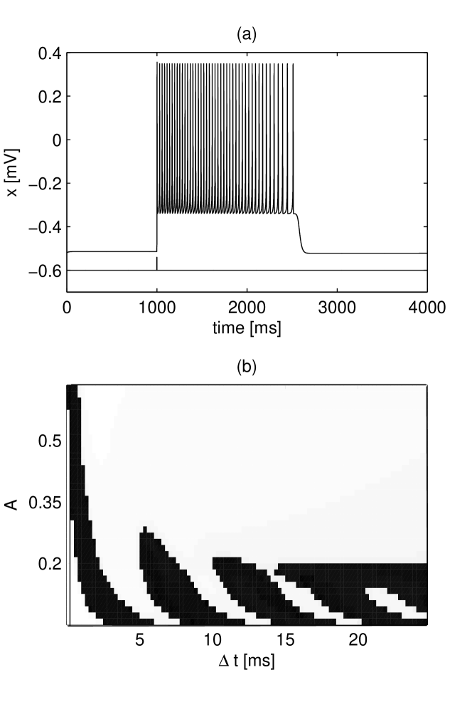
Figure 1: (a) Excitable burst (upper time series) evoked by noiseless external stimulation $S$ (lower time series plotted out of scale). (b) Response characteristics of the system to external stimulations of amplitude $A$ and duration $\Delta t$. White color corresponds to a single spike response, and black color corresponds to fixed duration bursts. In (a) and (b) the Morris-Lecar system with $c=0.28$ is considered.

In addition to the stochastic coherence, the phenomenon of stochastic incoherence (SI) has been reported, showing that in excitable systems exists a range of noise amplitudes at which the maximum inter-spike variability is observed. The phenomenon has been demonstrated in leaky integrate-and-fire model lindner where the mechanism of occurrence has been attributed to the third time scale existing in excitable systems, the absolute refractory period. SI has been also shown to occur in FitzHugh-Nagumo model sancho where the underlying mechanism has been associated with the nonmonotonous relaxational behaviour of the system near the oscillatory regime.

In this work a different type of stochastic incoherence is reported, namely, response stochastic incoherence (RSI). Its occurrence is found in a dynamical regime of excitable bursting. In the case of two dimensional excitable systems the spike duration (refractory period) is approximately fixed while the inter-spike interval is extremely sensitive to noise. In the case of bursting systems subject to noise, maximal variability is observed both in the inter-burst intervals and in burst durations. However, the two phenomena are observed in different range of noise amplitudes. In particular, the maximal variability in the inter-burst interval occurs for higher noise levels and refers to stochastic incoherence. In this study, the generation of bursts is triggered by a stimulus and not by the accompanying noise, whose only role is that of inducing variability in the duration of the elicited burst. It is shown, that the variability of excitable burst durations $T_{B}$ manifests a pronounced maximum at the optimal amplitude of fluctuations. The phenomenon is referred to as an incoherent in order to maintain a close relation with a well-known SI observed in excitable systems. The meaning of an incoherence in the case of RSI is associated with a maximum irregularity observed in $T_{B}$ as the noise intensity is varied. It is demonstrated that the mechanism of the variability maximization in response duration is mainly determined by the sensitivity of the system hysteresis, which determines bursting regimes, to noise. During a decrease of the mean burst duration, or equivalently, a decrease of the hysteresis depth, the system transforms from hard excitation state (hysteretic) into a soft excitation state (non-hysteretic), leading to a single spike mean responses at larger noise amplitudes. The maximum variability occurs when the symmetry breaking in the distributions for burst durations takes place. This symmetry breaking is caused by the existence of the minimum possible response length (single spike) which becomes highly probable at larger noise amplitudes. The occurrence of the phenomenon is demonstrated in the Morris-Lecar model equations. Its underlying mechanism is explained on examples of canonical systems containing hysteresis. In particular, in models describing stabilized subcritical pitchfork bifurcation (or subcritical Hopf bifurcation), and in a model describing a damped pendulum.

II Model

The general model equations are considered:

$$\{\epsilon_{1}\dot{x},\epsilon_{2}\dot{y},\epsilon_{3}\dot{z}\}=\{f(x,y,z)+S(t),g(x,y),h(x,z)\}$$ (1)

where $x-y$ is the fast subsystem and $z$ is the slow variable. The fast subsystem $x-y$ gives autonomous spiking, meanwhile variable $z$ rebounds spikes and enables bursting regimes, including excitable bursts. $S(t)$ is an external perturbation acting as an external stimulus provoking the excitable response of a neuron and has the form of the Dirac $\delta$ function. One chosen system parameter is then assumed to fluctuate following an independent white noise process $\xi(t)$ with correlations $\langle\xi(t)\xi(t^{\prime})\rangle=2D\delta(t-t^{\prime})$ and zero mean. The choice of the random process type is motivated by results reported in Ref. rowat which show that Gaussian noise has the same effect as channel or synaptic noise.

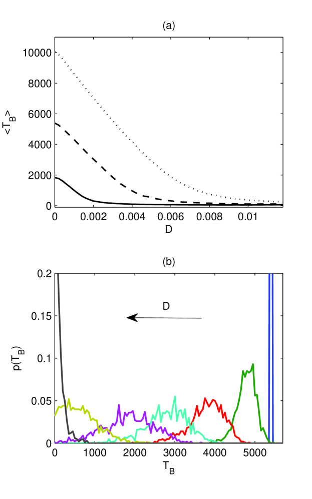
Figure 2: (a) Mean response durations for different values of the control parameter: $c=0.291$ (solid line), $c=0.326$ (dashed line) and $c=0.368$ (dotted line). (b) Normalized distributions of the response durations in the case of $c=0.326$ shown for increasing noise amplitudes (from right to left): $D=\{0,6\times 10^{-4},0.0014,0.0022,0.003,0.0046,0.0118\}$ (the distributions for $D=0$ and $D=0.0118$ are shown partially).

II.1 Rebound bursting in Morris-Lecar system

A special case of the general model in Eq. (1) is the modified Morris-Lecar model lecar :

$$\epsilon_{1}\dot{x} = \Gamma(x)-2y(x+0.7)-0.01z(x+0.885)+S(t)$$

$$\epsilon_{2}\dot{y} = c(-y+1/(1+e^{-(x-0.1)/0.07})$$

$$\epsilon_{3}\dot{z} = -z+9.3(x+0.6)$$ (2)

where $\Gamma(x)=-(1+e^{(-(x+0.01)/0.075)})^{-1}(x-1)-0.065(x+0.5)$, $\epsilon_{1}=0.97$, $\epsilon_{2}=1/\cosh((x-0.1)/0.14)$ and $\epsilon_{3}=30550$. The Morris-Lecar model is a conductance-based model of voltage oscillations in the barnacle giant muscle fiber which is often used as a qualitatively accurate model of neuronal spiking. In order to obtain a rebound burst, the additional variable $z$ is added to the subsystem $x-y$. An example of such a bursting response is shown in Fig. 1 (a). The system in Eq. (2) contains a dynamical hysteresis, i.e. a regime with transient bistability between a fixed point and repetitive spiking. The existence of such a dynamical hysteresis is responsible for bursting dynamics. The rest state disappears via fold bifurcation, and the periodic spiking disappears via saddle-homoclinic orbit bifurcation terman . The latter bifurcation allows class I neural excitability, since it manifests in low frequencies appearing at the transition to a rest state onset.

As already mentioned in the Introduction, the rebound bursting system has a rather pseudo-refractory period, since it can be influenced by the slight external fluctuations. On the other hand, the external stimulation has to be strong enough to elicit the rebound bursting response. Let consider the noiseless case when the system is stimulated with a rectangular single pulse of amplitude $A$ and duration $\Delta t$. Numerical simulations show that the system responses have a form of a fix duration burst or single spike. The nonlinear responses characteristics to such external stimulation are shown in Fig. 1 (b). It can be seen that the response of the system is bistable (coexistence of single spike and fixed duration bursting responses). A lack of variability in the burst durations and the two state responses of the system to stimuli with different parameters ($A$ and $\Delta t$) suggest, that the system is rather unsensitive to fluctuations in external stimulation eliciting excitable burst. As a consequence, only fluctuations present in an upper spiking state can give rise to a variability in the response durations. In the presence of noiseless stimulus $S$, the system fires a burst of a fixed duration, with a well-defined passage from the lower to the upper state and vice versa, determined by internal system parameters. In Eq. (2) the burst duration can be controlled by modulation of the parameter $c$.

II.2 RSI in rebound burster

Two cases are considered: i) the parameter $c$ is chosen to fluctuate $c\rightarrow c+D\xi(t)$, modelling the internal noise or ii) the stimulus $S$ is chosen to be accompanied by external fluctuations $S\rightarrow S+D\xi(t)$. The rebound bursting can be measured in different manners. One way is to estimate the total time during which the repetitive spiking takes place. Another way is to count the number of spikes in a given burst, as usually done in experiments experRebound . In the present work, the former way for measuring the burst durations $T_{B}$ is used, namely, the estimation of temporal intervals during which the system fires spikes repetitively. In order to describe qualitatively the variability of the response durations, standard deviation is considered $\sigma_{T_{B}}=(\langle T_{B}^{2}\rangle-\langle T_{B}\rangle^{2})^{\frac{1}{2}}$ where $\langle\rangle$ stands for mean. The statistical measurements are done on an ensemble of excited bursts in the presence of different realizations of noise. The noise intensities taken into consideration are small enough to keep $FAR=0$ (FAR-false alarm rate) at $S=0$. This is done in order to study the specific response of the system to external stimulation. It is observed, that the mean burst duration decreases with increasing of noise intensity. In Fig. 2 (a) the effect of noise on the mean burst duration for different values of the parameter $c$ is shown. This implies that in the presence of noise, the passage from the upper to the lower state becomes faster, and the transition time decreases as noise amplitude increases. The same behaviour is observed for both types of fluctuations present in the system. In view of the above results, it can be hypothesized that noise destroys the transiently existing bistability region in the bursting system, and transforms the hard excitation system into a standard excitable one-spike system or soft excitation system. This is clearly shown in Fig. 2 (b) where the distributions of the burst durations are plotted for different values of noise amplitude. From these distributions $\sigma_{T_{B}}$ is calculated and plotted in Fig. 3 (a) for various noise intensities $D$. The maximum of $\sigma_{T_{B}}$ corresponds to a maximum variation in excitable burst durations. The choice of $\sigma_{T_{B}}$ to describe the variability of $T_{B}$ instead of the usually used coefficient of variation $CV=\sigma_{T_{B}}/<T_{B}>$ is caused by the fact that $<T_{B}>$ decreases with the increase of $D$. Thus, having a division by decreasing quantity, $CV$ hides the useful information about $T_{B}$ variability. In fact, it has been already pointed out in lindner2002 , that $CV$ sometimes fails as an indicator of coherence.

It has been shown that the burst duration can be modified either by modulation of a control parameter $c$, either by varying the noise intensity. In fact, both, the effects of a control parameter $c$ and noise amplitude $D$ on the burst duration, are shown to be equivalent (see Fig. 3 (b)). This implies that random fluctuations in the rebound burster can play a role of a control parameter.

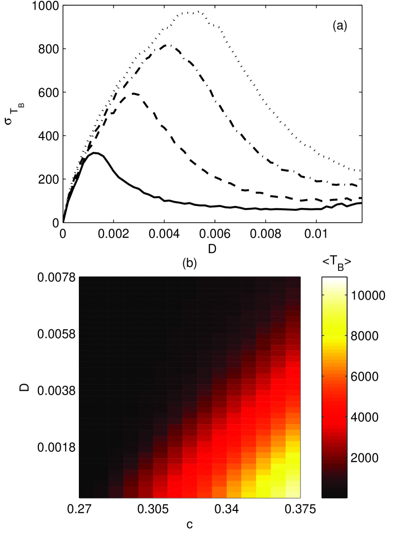
Figure 3: (a) Standard deviation $\sigma_{T_{B}}$ versus noise amplitude $D$ for different values of the control parameter: $c=0.291$, $c=0.319$, $c=0.347$ and $c=0.368$. (b) Dependence of $\langle T_{B}\rangle$ on noise amplitude $D$ and control parameter $c$.

III Mechanism of RSI

III.1 Sensitivity of hard excitation states to noise

In order to understand the effects of noise on the burst duration in the Morris-Lecar system let consider a canonical model of a system containing hysteresis which describes a stabilized subcritical pitchfork bifurcation strogatz :

$$\dot{x}=rx+x^{3}-x^{5}$$ (3)

In the case, when the additional subsystem equation $\dot{\phi}=2\pi$ is added to Eq. (3) and $x$ is considered as a radial variable, the system undergoes subcritical Hopf bifurcation mackey . In the absence of the stabilizing term $x^{5}$ the system in Eq. (3) undergoes a supercritical pitchfork bifurcation when one unstable fixed point bifurcates to three fixed points, one stable and two unstable. The stabilizing term allows the re-occurrence of the two stable and one unstable fixed points. The common feature between the saddle-node (occurring in the Morris-Lecar model) and stabilized subcritical pitchfork bifurcations is the existence of low frequencies (in the case of saddle-node bifurcation) or low amplitudes (in the case of pitchfork bifurcation) appearing at the bifurcation onset. The two backward-bending branches of unstable fixed points bifurcate from the origin when $r=r_{0}=0$. Due to a stabilizing term $x^{5}$, the unstable branches bend and become stable at $r=r_{s}$, where $r_{s}<0$. The stable large-amplitude branches exist for all $r>r_{s}$. In the range $r_{s}<r<0$, two different stable states coexist, the origin and the large-amplitude fixed points, which marks the hysteresis region. Inside this hysteretic region, the initial condition $x_{0}$ determines which fixed point is approached as $t\rightarrow\infty$. In the white noise environment, the following stochastic differential equation is obtained for Eq. (3):

$$dx_{t}=(rx_{t}+x_{t}^{3}-x_{t}^{5})dt+Dx_{t}dW_{t}$$ (4)

where the parameter $r$ is assumed to fluctuate as $r_{t}=r+D\xi_{t}$, where $r$ is an average value, $\xi_{t}$ is a Gaussian white noise and $D$ is the intensity of the fluctuations. Numerical simulations of Eq. (4) for different realization of noises reveal, that the same phenomenon as in the Morris-Lecar system occurs: the reduction of the mean hysteresis length (corresponding to the burst duration in the Morris-Lecar system) with increasing noise intensity. The bifurcation diagrams for a system with and without noise are shown in Fig. 4 (a) and the distribution of the hysteresis lengths $\Delta r$ for different noise amplitudes are plotted in Fig. 4 (b). The mean hysteresis lengths $\langle\Delta r\rangle$ calculated from the distributions reveal the monotonous decrease until they reach $\langle\Delta r\rangle=0$. The mean values and its standard deviations $\sigma_{\langle\Delta r\rangle}$ are shown in Fig. 4 (c). This implies the existence of a general mechanism of hysteresis reduction induced by noise.

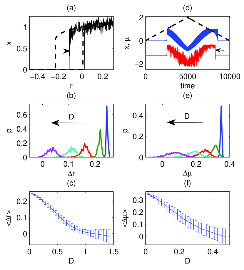
Figure 4: A canonical model for stabilized subcritical pitchfork bifurcation: (a) bifurcation diagram for a system without (dashed line) and with noise (solid line); the arrow marks the hysteresis reduction; (b) normalized distributions of the hysteresis lengths $\Delta r$ for selected noise amplitudes (from right to left): $D=\{0.0474,0.1897,0.3795,0.5218,0.8064\}$; (c) mean hysteresis length $\langle\Delta r\rangle$ and its standard deviation $\sigma_{\langle\Delta r\rangle}$. Model describing damped pendulum: (d) response of the system to a variation of internal parameter $\mu$ (dashed line); upper trace corresponds to the system without noise and the lower to the system with noise; the arrow shows the hysteresis reduction; (e) normalized distributions of the hysteresis lengths $\Delta\mu$ for selected noise amplitudes (from right to left): $D=\{0.0158,0.0632,0.1265,0.1897,0.3162\}$; (f) analogue to (c).

Another example of a system with hysteresis is the equation describing the dynamics of a pendulum with viscous damping (or a Josephson junction) strogatz :

$$\dot{\phi} = x$$

$$\dot{x} = \mu-\sin\phi-\alpha x$$ (5)

where $\alpha$ and $\mu$ are dimensionless control parameters. The parameter $\mu$ is assumed to fluctuate as $\mu_{t}=\mu+D\xi_{t}$, where $\mu$ is an average value, $\xi_{t}$ is a Gaussian white noise and $D$ is the intensity of the fluctuations. At small $\alpha$ and in the absence of noise ($D=0$), as the parameter $\mu$ is increased the initially stable fixed point disappears in a saddle-node bifurcation at $\mu=1$ giving a limit cycle. If $\mu$ is brought back down, the limit cycle persists for $\mu<1$ and its frequency tends to zero as $\mu=\mu_{c}$. This change in $\mu$ values as the bifurcation point is reached from different sides marks the hysteresis region. Now, when the internal parameter $\alpha$ is made fluctuating, the hysteretic region is seen to decrease with increasing noise amplitude (see Fig. 4 (d)). The same phenomenology of hysteresis reduction is observed also in this case (see Fig. 4 (e)). The averaged hysteresis depths $\langle\Delta\mu\rangle$ for different noise amplitudes are shown in Fig. 4 (f).

III.2 Existence of a minimum mean response duration in the bursting system

In the case of the Eqs. (3) and (5) the drift and diffusion processes continue until the averaged value $\langle\Delta r\rangle=0$ and $\langle\Delta\mu\rangle=0$ are reached, respectively. Then, when noise still increases, the drift disappears and only the amplitude of fluctuations around the states $\langle\Delta r\rangle=0$ and $\langle\Delta\mu\rangle=0$ increases (i.e. the diffusion increases with increasing $D$). In the case of a rebound burster, however, in which the hysteresis is a dynamic process allowing the transient spiking activity, the burst duration cannot be negative. Thus not only the drift stops but also the diffusion does. It occurs when the minimum possible burst duration $T_{B}^{min}$, being a single-spike response like in a standard excitable system, is reached (see Fig. 5 (a)). The maximum variance is observed when the distribution is situated in the intermediate distance between two stable states: single spike and a maximum rebound burst defined at $D=0$. Such a situation permits the system responses to visit all possible intermediate states giving the maximal variance. At larger noise amplitudes (but small enough to keep $FAR=0$), the single spike responses become more probable giving rise to a $T_{B}$ variability minimization. The value $T_{B}^{min}$ is a kind of a barrier which suppresses further increase of $\sigma_{T_{B}}$. The variability increases with $D$ until one tail of a distribution starts to disappear due to a collision with this barrier. In other words, the maximum variability of $T_{B}$ is associated with the symmetry breaking in the form of distributions for $T_{B}$’s consisting on the transitions from a normal to an exponential distribution form (see Fig. 2 (b)). The symmetry of the probability distributions can be measured by the skewness coefficient $\gamma_{1}$, the standardized moment, defined as follows:

$$\gamma_{1}=\frac{\mu_{3}}{\sigma_{T_{B}}^{3}}$$ (6)

where $\mu_{3}$ is the third moment about the mean $\langle T_{B}\rangle$ and $\sigma_{T_{B}}$ is the standard deviation. The skewness of the normal distribution (or any perfectly symmetric distribution) is zero. The symmetry breaking in the distributions described by skewness coefficient $\gamma_{1}$ is shown in Fig. 5 (b). The correlation between minimum of $\gamma_{1}$ (tendency to a normal distribution form) and maximum of $\sigma_{T_{B}}$ is clearly seen.

(a)

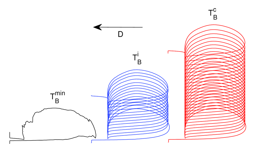
(b)

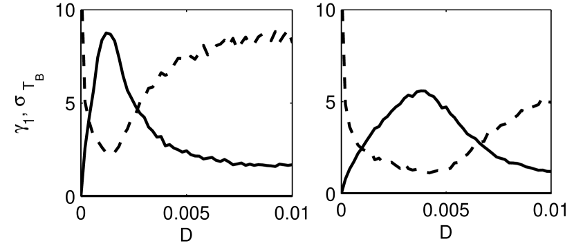
Figure 5: (a) Burst durations in the presence of noise: minimum possible $T_{B}^{min}$ (one spike) for $D=0.06$, intermediate $T_{B}^{i}$ for $D=0.005$ and in the absence of noise: $T_{B}^{c}$ determined by the value of parameter $c$, in this case $c=0.275$. (b) Correlation between the standard deviation $\sigma_{T_{B}}$ (solid line, plotted out of scale) and skewness $\gamma_{1}$ (dashed line). Left panel corresponds to Eq. 2 with $c=0.284$ and the right panel to $c=0.333$.

In the case of Eq. 5 describing the dynamics of a pendulum with viscous damping, the distributions for the hysteresis depth tend to be symmetric as the noise amplitude increases. This is indicated by the skewness coefficient shown in Fig. 6, which at difference to the case of the bursting system, remains small and constant.

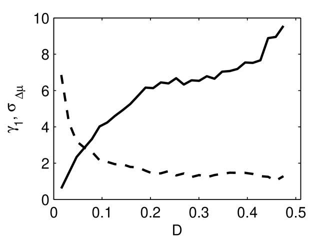
Figure 6: Correlation between the standard deviation $\sigma_{\Delta\mu}$ (solid line, plotted out of scale) and skewness $\gamma_{1}$ (dashed line) in the case of the equation describing the dynamics of a pendulum with viscous damping (Eq. 5).

IV Discussion

In this work the phenomenon of response stochastic incoherence in rebound bursters has been reported. The crucial ingredients for RSI to appear are the existence of hysteresis in the system and at least three dimensions, allowing a fast-slow configuration and rebound bursting regime. The underlying mechanism has been provided, showing that the maximum variability in burst durations is caused by the sensitivity of the system hysteresis responsible for bursting dynamics to noise and by the symmetry breaking in distributions for the burst durations occurring as the barrier situated at the minimum value of the response duration (single spike response) is reached. The hysteresis vulnerability to noise has been demonstrated on examples of canonical systems describing hard excitation states. The implications of this finding is that the bursting responses to external stimulation are not necessarily well-determined and fixed, but depend strongly on the slight presence of random fluctuations. From the physical point of view the phenomenon of RSI here presented regards a different kind of stochastic incoherence, namely, the variance of the burst durations instead of interspike intervals as reported so far in the literature.

The results on the hysteresis reduction could contribute to the understanding of some phenomena observed in models for bursting dynamics like the decreasing burst durations in the presence of noise pancreas . On the other hand, RSI may be relevant in asynchronous firing patterns as already proposed for the case of SI in Ref. 30 .

References

References

- (1) W. Horsthemke and R. Lefever, Noise-Induced Transitions. Theory and Applications in Physics, chemistry, and Biology, Springer Series in Synergetics, 2006.
- (2) L. Gammaitoni, P. Hänggi, P. Jung, and F. Marchesoni, Rev. Mod. Phys. 70 (1998) 223.
- (3) B. Lindner, J. Garc a-Ojalvo, A. Neiman, and L. Schimansky-Geier, Phys. Rep. 392 (2004) 321.
- (4) K. Wiesenfeld, D. Pierson, E. Pantazelou, C. Dames, and F. Moss, Phys. Rev. Lett. 72 (1994) 2125; F. Marino, M. Giudici, S. Barland, and S. Balle, Phys. Rev. Lett. 88 (2002) 040601.
- (5) R. Benzi, A. Sutera, and A. Vulpiani, J. Phys. A 14 (1981) 453; C. Nicolis and G. Nicolis, Tellus 33 (1981) 225.
- (6) H. Gang, T. Ditzinger, C. Z. Ning, and H. Haken, Phys. Rev. Lett. 71 (1993) 807.
- (7) A. S. Pikovsky, and J. Kurths, Phys. Rev. Lett. 78 (1997) 775.
- (8) F. Sagues, J. M. Sancho, and J. Garcia-Ojalvo, Rev. Mod. Phys. 79 (2007) 829.
- (9) K. Pakdaman, S. Tanabe, and T. Shimokawa, Neural Networks 14 (2001) 895.
- (10) A. Neiman, P. I. Saparin, and L. Stone, Phys. Rev. E 56 (1997) 270.
- (11) A. Longtin, Phys. Rev. E 55 (1997) 868.
- (12) S. Wu, W. Rend, K. He, and Z. Huang, Phys. Lett. A 279 (2001) 347.
- (13) G. Zhang, J. Xu, J. Wang, Z. Yue, C. Liu, H. Yao, and X. Wang, Advances in Cognitive Neurodynamics ICCN pp. 83-89, 2007.
- (14) L. I and J. M. Liu, Phys. Rev. Lett. 74 (1995) 3161.
- (15) G. Giacomelli, M. Giudici, S. Balle, and J. R. Tredicce, Phys. Rev. Lett. 84 (2000) 3298.
- (16) C. S. Zhou, J. Kurths, E. Allaria, S. Boccaletti, R. Meucci, and F. T. Arecchi, Phys. Rev. E 67 (2003) 066220.
- (17) E. M. Izhikevich, Int. J. Bif. Chaos 10 (2000) 1171.
- (18) R. FitzHugh, Biophys. J. 1 (1961) 445; J. Nagumo, S. Arimoto, and S. Yoshizawa, Proc. IREE aust. 50 (1962) 2061.
- (19) B. Lindner, L. Schimansky-Geier, and A. Longtin, Phys. Rev. E 66 (2002) 031916.
- (20) A. M. Lacasta, F. Sagues, and J. M. Sancho, Phys. Rev. E 66 (2002) 045105(R).
- (21) P. Rowat, and R. Elson, J. Comput. Neuroscience 16 (2004) 87.
- (22) C. Morris and H. Lecar, Biophys. J. 35 (1981) 193-213.
- (23) D. Terman, SIAM J. Appl. Math. 51 (1991) 1418.
- (24) W. Zhang, J. H. Shin, and D. J. Linden, J. Physiol 561.3 (2004) 703 719.
- (25) B. Lindner, A. Longtin, and A. Bulsara, Neural Comput. 15 (2003) 1760.
- (26) S. H. Strogatz, Nonlinear dynamics and chaos: with applications to physics, biology, chemistry and engineering, Addison-Wesley Publishing Company, 1997.
- (27) L. Glass, and M. C. Mackey, From clocks to chaos. The rhythms of life, Princeton University Press, 1988.
- (28) T. R. Chay and H. S. Kang, Biophys. J. 54 (1988) 427-435.