Statistical distributions of quasi-optimal paths in the traveling salesman problem:
the role of the initial distribution of cities.

Abstract

Solutions to Traveling Salesman Problem have been obtained with several algorithms. However, few of them have discussed about the statistical distribution of lengths for the quasi-optimal path obtained. For a random set of cities such a distribution follows a rank 2 daisy model but our analysis on actual distribution of cities does not show the characteristic quadratic growth of this daisy model. The role played by the initial city distribution is explored in this work.

Keywords: Traveling Salesman Problem, city distribution, statistical properties.

Las soluciones al Problema del Agente Viajero han sido obtenidas con varios algoritmos. Sin embargo, poco se ha discutido sobre la distribución de longitudes para el camino cuasi-optimal obtenido. Para un conjunto al azar de ciudades esta distribución sigue un modelo margarita de rango 2, pero nuestro análisis sobre distribuciones reales de ciudades no muestra el crecimientos cuadrático característico de este modelo margarita. En este trabajo se explora el rol jugado por la distribución inicial de ciudades.

Descriptores: Problema del Agente Viajero, distribución de ciudades, propiedades estadísticas.

I Introduction

Statistical approaches to complex problems have been successful in a wide range of areas, from complex nuclei Wigner to the statistical program for complex systems (see for instance Ref. Palis ), including the fruitful analogies with statistical mechanics. The main goal is to find universal properties, i.e., properties that do not depend on the specifics of the system treated but on very few symmetry or general considerations. An example of such an approach is represented by the Random Matrix Theory (RMT) Mehta3ed ; WeidenmullerGuhr which has been applied successfully to wave systems in a range of typical lengths from one femtometre to one metre.

Attempts to apply a RMT approach to a non-polynomial problem like the Euclidean Traveling Salesman problem (TSP) is not the exception Flores ; hhs . For an ensemble of cities, randomly distributed, general statistical properties appear and they are well described for a daisy model of rank $2$hhs . However, in realistic situations the specific system seems to be important, as we shall see later, and the initial conditions rule the statistical properties of the solutions. In the present work we deal with a similar analysis both for actual TSP maps for several countries through the planet and for some toy models that could help to understand the role of initial conditions in the transition to universal statistical properties. An interesting link appears with the distribution of corporate vote when we map the lengths in the TSP problem to the number of votes, after a proper normalization.

The paper is organized as follows: In section II we define the TSP and the statistical measures we shall use. Special attention will be paid to the separation of secular and fluctuation properties. Here, we analyze maps of actual countries. In section III we discuss the transition from a map defined on a rectangular grid to a randomly distributed one using two random perturbations to the city positions: i) a uniform random distribution with a width $\sigma$ and, ii) a Gaussian distribution. In the same section, we discuss the relation of the latter toy model to the distributions of corporate vote. The conclusions appear in section IV.

II Statistical properties of quasi-optimal lengths

In the Traveling Salesman Problem a seller visits $N$ cities with given positions $(x_{i},y_{i})$, returning to her or his city of origin. Each city is visited only once and the task is to make the circuit as short as possible. This problem pertains to the category of so called NP-complete problems, whose computational time for an exact solution increases as an exponential function of $N$. It is, also, a minimization problem and it has the property that the objective function has many local minima NumericalRecipes .

Several algorithms exist in order to solve it and the development of much more efficient ones is matter of current research. Since we are interested in statistical properties of the quasi-optimal paths, small differences between the different algorithms are not of relevance and we shall consider all of them as equivalent. The computational time is irrelevant as well. In this paper we used the results of Concorde Concorde for the actual-country TSP, and simulated annealing NumericalRecipes and 2-optimal Croes for the analysis of specific models.

The first step in the analysis consist in separating the fluctuating properties from the secular ones in the data. This process could be nontrivial WeidenmullerGuhr . The idea behind this procedure is that all the peculiarities of the system resides in the secular part and the information carried out by the fluctuations have an universal character. In the energy spectrum of many quantum systems, when almost all the symmetries are broken, this kind of analysis has shown that the fluctuations are universal and regarding only to the existence or not of a global symmetry like time reversal invariance. The peculiarities of the system, wheather it is a many particle nucleus, an atom in the presence of a strong electromagnetic field, or a billiard with a chaotic classical dynamics, all these characteristics are in the secular part WeidenmullerGuhr . In the present case, we assume that the dynamics that rules where the cities are located is sufficiently complex in order to admit this kind of analysis. If not, as we shall see later, the next step in our analysis is to search for the reason of such a lack of universality.

In order to perform this separation we consider the density of cumulative lengths, $d$, named

$$\rho(d)=\sum_{k}\delta(d-d_{k}),$$

with $\delta(\cdot)$, the Dirac’s delta function. The cumulative lengths $d_{k}$ are ordered as they appear in the quasi optimal path and are defined as $d_{k}=\sum_{i=1}^{k}l_{i}$ with $l_{i}=\sqrt{(x_{i}-x_{i-1})^{2}+(y_{i}-y_{i-1})^{2}}$ being the length between city $i-1$ and $i$. The cities are located at $(x_{i},y_{i})$ in the $X-Y$ plane. The corresponding cumulative density is

$${\cal N}(d)=\sum_{k}\Theta(d-d_{k}),$$

with $\Theta(\cdot)$, the Heaviside function. The task is to separate ${\cal N}(d)$ as ${\cal N}_{Secular}(d)+{\cal N}_{fluctuations}(d)$. The secular part is calculated using a polynomial fitting of degree $n$. After this, we consider as the variable to analyze the one mapped as

$$\xi_{k}={\cal N}_{Secular}(d_{k}).$$

We shall study the distributions of the set of numbers ${\xi_{k}}$. Notice that this transformation makes that $\langle\xi\rangle=1$. The analysis is performed on windows of different size, this kind of analysis is always of local character. For historical reasons this spreading procedure is named unfolding. From all the statistics we shall focus on the nearest neighbor distribution, $P(s)$, with $s_{i}=\xi_{i}-\xi_{i-1}$ (which is the normalized length), and the number variance, $\Sigma^{2}(L)$, for the short and large range correlations, respectively. The $\Sigma^{2}(L)$ is the variance in the number of levels $\xi_{n}$ in a box of size $L$, see Mehta3ed ; WeidenmullerGuhr for a larger explanation.

The actual maps considered in this work were those which are reported in Concorde’s web page Concorde , and we selected those that have a number of cities larger than $1000$ and present no duplications. The countries selected are reported in table 1.

	Name	N cities	$l_{max}$	$<l>$
1	Burma	33708	8650.00	197.00
2	Canada	4663	76133.33	10263.28
3	China	71009	51646.00	4225.62
4	Egypt	7146	6708.34	431.90
5	Ireland	8246	4059.17	973.62
6	Finland	10639	10200.01	536.04
7	Greece	9882	6600.02	286.97
8	Italy	16862	10050.00	438.46
9	Japan	9847	16166.68	581.44
10	Kazakhstan	9976	38925.00	5559.56
11	Morocco	14185	8056.41	418.08
12	Oman	1979	3685.56	541.17
13	Sweden	24978	9250.02	368.03
14	Tanzania	6117	10166.68	1145.41
15	Vietnam	22775	4983.36	145.26
16	Yemen	7663	10810.28	877.26

Table 1: Countries considered for the study. The quasi-optimal path was obtained from the web page in Ref. Concorde . Maximum and average length (in km) are reported too.

The results in the ${\cal N}(l)$ are full of variations, as expected. The secular part was calculated with several windows size and polynomial degrees looking for those parameter values that stabilize the statistics. However, a no universal behavior appears. The graphs presented in Fig. 1 for the nearest neighbor distribution were calculated using a polynomial fitting of fourth degree and windows of $200$ lengths, the histograms have a bin of size $0.004$. There we show the distribution for all the countries in table 1. There is no a single distribution even when some of the countries show a exponential decay as occurs with Finland (see Fig. 2). We analyzed the data with several windows size and polynomial degrees with similar results.

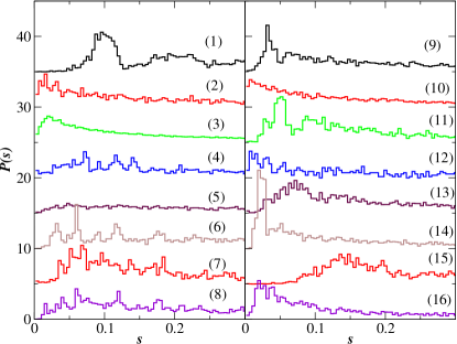
Figure 1: (color online) Nearest neighbor distribution of normalized lengths (histogram), for the quasi-optimal path in the countries referred in Table 1. For sake of clarity, we shifted the distributions. The bin size is $0.004$ and notice that the normalized average is $s=1$.

No regularities were found in our analysis but all the histograms show almost a maximum and some of them present a polynomial grow, $s^{\alpha}$, at the beginning of the distribution. This could be seen in Burma (1), Japan (2) and Sweden (13). Notice that the distributions present the maximum at $s<0.2$ meanwhile the average is at $s=1$. Hence, all the distributions present a long tail. However the type of decay is diverse as well (see Fig. 2). Some distributions present a clear exponential decay, like Finland. Some others present a mixed decay as is the case of China. For sake of clarity we do not show all the cases in Fig. 2. Notice that the bin size is larger in Fig. 2 compared to that used in Fig. 1, for this reason, the polynomial grow does not appear.

We try to show countries of several sizes and urban configurations. There are some countries with an urban density almost constant, like Sweden, and some others with long tails and a maximum for very short distances as Canada. Changes in the parameters of analysis, windows size and fitting polynomial degree, do not give us an universal behavior. Recall that this is not the case for an ensemble of randomly distributed cities as seen in Ref.Flores ; hhs . From all these results it is clear that the initial distribution of cities plays a crucial role in the final quasi-optimal result. This is the subject of the next section.

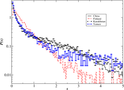
Figure 2: (color online) Nearest neighbor distribution of normalized lengths in semi-log scale, for the quasi-optimal path in the countries referred in the inset. The bin size is $0.04$.

III The role of the initial distribution of cities

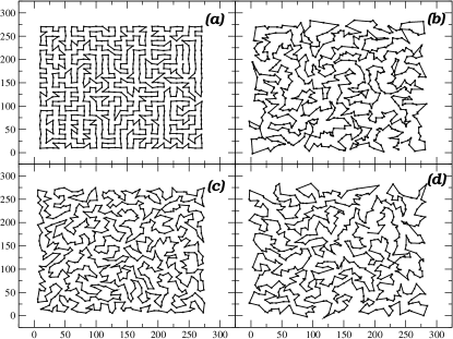
Figure 3: Examples of the quasi-optimal path on one map of the model I, with values of (a)$\sigma=1.0$ and (b)$\sigma=15.0$. For model II, the considered values are (c) $\sigma=5.0$ and (d) $\sigma=10.0$. The maps consist of $27\times 27$ cities.

The statistical properties of quasi-optimal paths for an ensemble of randomly distributed cities in the Euclidean plane is well described by the so called daisy model of rank $r=2$ hhs . These models are the result of retaining each $r+1$ number from a sequence of random numbers $y_{i}$ which follow a Poisson distribution, i.e, its $n$-nearest neighbor distribution has the form

$$P(n,s)=\frac{s^{n-1}}{(n-1)!}\exp(-s),$$

with $s_{i}=y_{i+n}-y_{i}$ and $n=1$ corresponds to first nearest neighbors. The rarefied sequence must be re-scaled in order to recover the norm and the proper average of the $n$-nearest neighbor distributions.

For the general daisy model of rank $r$ we have the following expression for the nearest neighbor distribution:

$$P_{r}(s)=\frac{(r+1)^{(r+1)}}{\Gamma(r+1)}s^{r}\exp(-(r+1)s),$$ (1)

and,

$$\begin{split}\Sigma^{2}_{r}(L)=\frac{L}{r+1}+\frac{r(r+2)}{6(r+1)^{2}}+\frac{2}{(r+1)^{2}}\sum^{r}_{j=1}\frac{W_{j}}{(1-W_{j})^{2}}\\ \times\exp\left[(W_{j}-1)(r+1)L)\right],\end{split}$$ (2)

for the number variance. Here $W_{j}=\exp(2\pi ij/(r+1))$ are the $r+1$ roots of unity and $i$ stands for $\sqrt{-1}$.

In the case of $r=2$, both, the nearest neighbor distribution and the $\Sigma^{2}_{2}$ statistics have the theoretical results, namely

$$P_{2}(s)=\frac{3^{3}}{2!}s^{2}\exp(-3s),$$ (3)

and

$$\Sigma^{2}_{2}(L)=\frac{L}{3}+\frac{4}{27}\left[1-\cos(\frac{3\sqrt{3}}{2})\exp(-\frac{9}{2}{}L)\right].$$ (4)

As mentioned above, quasi-optimal paths of an ensemble of maps with cities randomly distributed nearly follow equations (3) and (4). Again, the final distribution of lengths in the quasi-optimal paths depends on the initial distribution of cities.

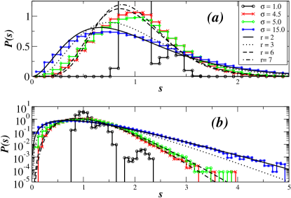
Figure 4: (color online) (a) Nearest neighbor distribution, $P(s)$, of normalized lengths for model I for the value of the $\sigma$ indicated in the key. The functions in continuous line and labeled with $r$ correspond to the distributions of the daisy model of equation 1. (b) Same as (a) but in semi-log scale. Note that the histogram for $\sigma=b/2=5.0$ is well fitted by the daisy model with $r=6$.(See text for details)

In order to understand the role of initial distribution of cities, we depart from a master map of cities on a square grid of side $b$, where the initial position of each city is in the intersections. In this case, the distribution of lengths for the quasi-optimal path is close to a delta function with a small tail. Now, we take an ensemble of maps, each one is built up relocating the cities from their original positions using a probability distribution of width $\sigma$, ${\cal P}(\sigma)$. That is

$$x_{i}=nb+p_{i}$$ (5)

$$y_{i}=mb+q_{i},$$ (6)

where the numbers $p_{i}$ and $q_{i}$ are taken from ${\cal P}(\sigma)$ which have zero mean and $n$ and $m$ are integers. Two distributions were selected, i) a uniform one with width $\sigma$, that we call model I, and ii) a Gaussian one with the same width, that we named model II. In Figure 3 several examples are shown of the quasi-optimal paths. The starting grid or master rectangle defining the $27\times 27$ cities is similar to that of Figure 3(a).

The distribution of lengths shows a transition from the original one to the limit case given by equations (3) and (4) as can be seen in Fig. 4 for a uniform distribution and in Fig. 5 for the Gaussian one. In these figures we plot $P(s)$ in both (a) linear and (b) logarithmic scale. The analysis was performed on an ensemble of $500$ maps of $27\times 27$ cities each. The variable $\sigma$ was considered in the interval $[0,15]$. Only relevant values are reported.

For model I, we plotted the histograms for $\sigma=1,4.5,5$ and $15.0$ (see Fig.4). For the first case the distribution departs barely from the initial one but, the quasi optimal solution presents a revival for $s$ slightly below $\sqrt{2}$(Fig. 4(a) the black histogram with circles), and for values slightly larger than $2$ representing the existence of diagonal lengths in the grid and lengths of order two $b$’s (in this uncorrelated variable, see Fig. 3(a)). The histograms show a continuous transition to the distribution given by Eq. (3) when $\sigma=15$ (blue histogram with stars). The tail, in this case, follows very closely the daisy model of rank 2 to it and the start of $P(s)$ is consistent with it (see Fig. 4(b)). The histogram in red with crosses corresponds to $\sigma=4.5$ and follows very closely the daisy model of rank $7$. Meanwhile, the histogram in green with diamonds, corresponding to $\sigma=5.0$, follows the rank $6$ model. The second case corresponds to the value of $\sigma$ when the distribution of the cities start to admit overlapping, i.e $\sigma=b/2$. When $\sigma=b$ the histogram coincides with the daisy model of rank $3$ (not shown).

For model II there exists a transition and the fitting to a daisy model is, as well, defined as in model I. In Fig. 5 we plot the cases $\sigma=5.0$ and $10.0$ which are close to daisy models of rank $3$ and $2$, respectively. In Fig. 5(b) we re-plotted in semi-log scale in order to see the tail decay. The interpretation is the same as the previous one. Fluctuations in the tails for large values of $\sigma$ are observed in the Gaussian case. The reason for them is that the map admits cities positioned far away from the master rectangle (not shown). Certainly, a fit using Weibull or Brody distributions is possible for both models, however it does not exist a link with any physical model whereas the daisy models are related to the 1-dimensional Coulomb problem hhs .

Figure 5: (color online) In the same order as previous figure, but for model II and the values of $\sigma$ and $r$ indicated. Notice that this time the value $\sigma=b/2=5.0$ is fitted by a daisy model or rank $r=3$.

An interesting link exists in this context between the distribution of lengths in the quasi-optimal path and the vote distribution trough Daisy models. In Ref. hhse1 it has been established that the distribution of corporate vote in Mexico, during elections from $2000$ to $2006$ follows a daisy model with ranks from $r=2$ to $r=7$. In the present case, exponential decays that are compatible with $r=3$ occur at $\sigma=b$ for model I and $\sigma=b/2$ for model II, i.e., $\sigma=10.0$ for the former and $\sigma=5.0$ for the latter. In both cases, distributions of the random perturbation overlap is significant. Other links look possible and are under consideration. This behavior remains poorly understood, but it opens new questions about the relationship between statistical mechanics problems and social behavior.

In the case of long range behavior, the analysis with the $\Sigma^{2}$ statistics looks promising, but the asymptotic behavior does not coincide with daisy models. This statistics is highly sensitive to the unfolding procedure described before. Wider studies are currently in progress, however we give in advance that the $\Sigma^{2}$ statistics for model I at $\sigma=15.0$ is close to that of the daisy model of rank 2. The slope is $0.317486\pm 7.31\times 10^{-5}$ which is close to the $1/3$ value obtained for the daisy model. For both models the $\Sigma^{2}$ starts following the behavior of Eq. (4). For small values of $\sigma$ the numerical results show an oscillatory behavior compatible with the presented in the daisy model, Eq. (2), even when the asymptotic slope is not the correct one.

IV Conclusions

We presented a statistical approach to the Traveling Salesman problem (TSP). No universal behavior appears in the case of actual distribution of cities for several countries world wide as it appears in the case of the Euclidean TSP with a uniform random distribution of cities Flores ; hhs . As a first step to understand the role of the initial distributions of cities, we study the nearest neighbor distribution for the lengths of quasi-optimal paths for a model which start with a periodic distribution of cities on a grid and it is perturbed by a random fluctuation of width $\sigma$. We use two models for the fluctuation: model I, a uniform distribution and, model II, a Gaussian one. Both models evolve, as a function of $\sigma$, from a delta like initial distribution to one well described by a daisy model of rank $2$ (see Eq. (3)). As the perturbative distribution width is increased the evolution of the models present a nearest neighbor distributions compatible with several ranks of the daisy model. Two values of the width are important, the first one is when the random perturbation admits an overlap of the cities originally at the periodic sites. For model I that occurs when $\sigma=b$ (the total width of the distribution is $2\sigma$), being $b$ the distance of the periodic lattice. For model II that happens when $b=2\sigma$, i.e. two standard deviations of the Gaussian distribution. In these cases the histogram of lengths fits a rank $3$ daisy model. An interesting link appears when we notice that such a daisy model fits the tail of the distribution of votes (for the chambers) for a corporate party in Mexico during election of 2006. The reason of this coincidence remains open and requires further analysis. An attempt in this direction is presented in Ref.hhs2010 . Another open question concerns about if an ensemble of world wide countries have universal properties or not. This topic is in current research.

References

- (1) E.P. Wigner. Proc. Cambridge Phil. Soc. 47 (1951) 790.
- (2) J. Palis Jr. Dynamical Systems and Chaos, Vol.1, (Singapore, World Scientific, 1995). p 217-225.
- (3) M. L. Mehta. Random Matrices. 3rd. ed. (Amsterdam, Elsevier, 2004).
- (4) T. Guhr,A. Müller-Groeling, and H.A. Weidenmüller. Phys. Rep. 299 (1998) 190.
- (5) R.A. Méndez, A. Valladares, J. Flores, T.H. Seligman, and O. Bohigas. Physica A 232(1996) 554.
- (6) H. Hernández-Saldaña, J. Flores and T.H. Seligman. Phys. Rev. E. 60 (1999) 449.
- (7) W.H. Press. S.A. Teukolsky, W.T. Vetterling, B.P. Flannery. Numerical Recipes. The art for Scientific Computing. 3rd. ed. ( N.Y., Cambridge Univ. Press, 2007).
- (8) D. L. Applegate, R. E. Bixby, V. Chvatal, W. Cook The Traveling Salesman Problem: A Computational Study. ( Princeton University Press, 2006). Chapter 16. http://www.tsp.gatech.edu/world/countries.html
- (9) G.A. Croes. Op. Research 6(6) (1958) 791-812.
- (10) H. Hernández-Saldaña.Physica A 388 (2009) 2699-2704.
- (11) H. Hernńandez Saldaña. Traveling Salesman Problem. Theory and Applications. D. Davendra, ed. (India, INTECH, 2010) pp. 283-298.