Shape Splines and Stochastic Shape Evolutions:
A Second Order Point of View

Abstract.

This article presents a new mathematical framework to perform statistical analysis on time-indexed sequences of 2D or 3D shapes. At the core of this statistical analysis is the task of time interpolation of such data. Current models in use can be compared to linear interpolation for one dimensional data. We develop a spline interpolation method which is directly related to cubic splines on a Riemannian manifold. Our strategy consists of introducing a control variable on the Hamiltonian equations of the geodesics. Motivated by statistical modeling of spatiotemporal data, we also design a stochastic model to deal with random shape evolutions. This model is closely related to the spline model since the control variable previously introduced is set as a random force perturbing the evolution.

Although we focus on the finite dimensional case of landmarks, our models can be extended to infinite dimensional shape spaces, and they provide a first step for a non parametric growth model for shapes taking advantage of the widely developed framework of large deformations by diffeomorphisms.

1. Introduction

Mathematical and statistical modeling of shapes has undergone significant development over the past twenty years driven by a wide range of applications in medical imaging. Initially the focus was on the comparison between two shapes also refereed to as registration. Among others, registration and comparison tools derived from a Riemannian point of view on shapes spaces and diffeomorphic transport have been actively developed during the past few years. This framework was used to represent shapes and study the statistical variation of static shapes within a population. An emerging question of interest is now to study time dependent data of shapes (images, landmarks, surfaces or tensors). The basic dataset is then a sequence of shapes indexed by time. For example, a practical application would be the analysis of follow-up studies in brain imaging.

Several attempts models for the variability of longitudinal data have been proposed recently: a parametric model of growth is proposed in [14, 15], which aims to describe the biological evolution as an iteration of random elementary diffeomorphisms, so called GRID. Focusing on image data, statistical estimation of the parameters are performed with the GRID model in [30, 32]. Other attempts are often based on using an initial registration tool (such as geodesics on a group of diffeomorphisms, see [35] for a large overview) to interpolate the time dependent data with piecewise geodesics [9, 22]. In [9], the model is further developed with the introduction of time realignments to allow the study of an ensemble of longitudinal data and the computation of an averaged space-time evolution.

From the modeling point of view a typical growth evolution is usually smooth in time. However, the piecewise geodesic models underlying current analysis of time dependent shape data can not prevent a loss of regularity at the observation points. Moreover, from a more classical statistical point of view, piecewise linear regression does not provide the best interpolation framework and from a probabilistic point of view the limiting process underlying piecewise geodesic interpolation is more or less a Kunita flow [23] that has a Brownian like time evolution. These remarks suggest that a better model of interpolation in time should be of higher order than piecewise geodesics, and also closely related to a probabilistic model of random evolution of shapes. The question of time interpolation was addressed in [7] with the use of a kernel on the time variable but still with underlying piecewise geodesics on the data. Random evolutions of shapes have been treated for instance in [8, 21], but here again the model is of first order in the sense that the evolution is not smooth in time.

In this work, we present a second order model for deterministic and stochastic shape evolution as a primary step toward further statistical applications. This work will extensively use the Hamiltonian framework that emerged several years ago in the field of Computational Anatomy (CA) to compute the registration of landmarks (points of interest on an image) [13, 19, 26]. This problem of landmark registration is equivalent to finding geodesics on the Riemannian manifold of landmarks. Thus shooting methods as well as gradient descent have been applied to solve this problem [4, 28].

A first natural step to deal with random shape evolution is to study a stochastic perturbation of the Hamiltonian equations of geodesics. If we consider the evolution of landmarks as a physical system of particles, it corresponds to the introduction of a random force on their evolution providing smooth time random perturbation around a mean geodesic trajectory. However, this in turn leads to a new deterministic counterpart when the stochastic term in the evolution of the momentum is replaced by a deterministic control variable. Given a sequence of time-indexed shapes, and optimizing on the control variable, we end up with a framework for smooth time interpolation between shapes. In the finite dimensional case of landmarks, this approach is directly related to splines on a Riemannian manifold [6, 29, 18, 5]. We will present a Hamiltonian approach to derive the equations for the splines in a Hamiltonian setting. It can be related to the work of [17] since they use a control point of view to obtain the Hamiltonian equations but our approach differs from theirs in that we use the Hamiltonian formulation of geodesics on landmark space. Hence there is a straightforward generalization to other Hamiltonian systems. The possible extension of the Hamiltonian equations of geodesics to curves, surfaces (or embeddings of manifolds in $\mathbb{R}^{n}$) is the key feature to design second order models of evolution on continuous shape spaces [13, 26, 34] but in this work we will concentrate on the finite dimensional case of landmarks. Note however, that contrary to the initial context of air-craft trajectory planning (where the target manifold is the low-dimensional Lie Group $\mathrm{SE}(3)$ - the Special Euclidean group on $\mathbb{R}^{3}$), for which splines on Riemannian manifold were introduced - shape spaces in Computational Anatomy are more strongly connected with the infinite dimensional case. Moreover, we will consider both the deterministic and the stochastic setting since these are considered as fundamental ingredients towards statistical analysis of longitudinal data.

The plan of the paper is as follows: we first introduce in section 2 the Hamiltonian equations for the case of landmarks, which constitute the central tool in this article. The section 3 is devoted to the spline model with different metrics and section 4 gathers theoretical results about the global existence in time of the second order deterministic spline evolution, the existence of a minimizer for the spline estimation problem and the derivation of the Euler-Lagrange equations. Then in section 5, we present some numerical experiments about shape spline estimation on 2D shape evolution, highlighting some of their main features. In section 6, we turn to problem of stochastic second order spline evolutions with a proof of the well-posedness and global existence in time and a few illustrative simulations. Last we develop in section 7 a slightly more general picture of shape splines on homogeneous spaces extending the model beyond the landmark setting.

2. Hamiltonian equations of geodesics for landmark matching

The problem of landmark matching via diffeomorphic transport is now quite well understood. The basic idea is to build a continuous path of minimal length $\phi_{t}$ starting from $\phi_{0}=\mathrm{Id}_{\mathbb{R}^{d}}$ in a group $G_{V}$ of diffeomorphisms, between an initial configuration $x=(x_{i})_{1\leq i\leq n}$ of $n$ landmarks in $\mathbb{R}^{d}$ and a target configuration $y=(y_{i})_{1\leq i\leq n}$ . Thus, if $x_{i,t}\doteq\phi_{t}(x_{i})$ and $x_{t}=(x_{i,t})_{1\leq i\leq n}$, $x_{t}$ is a path from $x$ to $y$ in the space of landmark configurations induced by a geodesic in a Riemannian space of diffeomorphisms. The group $G_{V}$ is defined through the flow of time dependent velocity fields $(t,x)\to v_{t}(x)$ on $\mathbb{R}^{d}$

(1) $$\frac{\partial\Phi}{\partial t}=v_{t}\circ\Phi$$

where $V$ is a Hilbert space of velocity fields and $v\in L^{2}([0,1],V)$ is an element of the space of time dependent velocity fields with finite $L^{2}$ norm. Obviously, the existence of a flow $t\to\Phi^{v}_{t}$ for $v\in L^{2}([0,1],V)$ solution of (1) depends on some regularity assumptions of the instantaneous velocity fields $v_{t}$, mainly the control of the first order derivatives of $v_{t}$. Assuming this, the group $G_{V}$ is defined as $G_{V}\doteq\{\Phi^{v}_{1}\ |\ v\in L^{2}([0,1],V)\}$ and the diffeomorphic matching problem for landmarks is formulated through the following variational problem

(2) $$\left\{\begin{array}[h]{l}\min\int_{0}^{1}|v_{t}|_{V}^{2}dt,\ v\in L^{2}([0,1],V)\\ \text{with}\\ \Phi^{v}_{1}(x_{i})=y_{i},\ 1\leq i\leq n\,.\end{array}\right.$$

The problem (2) is well posed as soon as $V$ is continuously embedded in $C^{1}_{0}(\mathbb{R}^{d},\mathbb{R}^{d})$ the space of $C^{1}$ velocities vanishing at $\infty$ (such a $V$ is called an admissible space). Namely, we assume the existence of a constant $C$ such that for any $v\in V$, the following inequality is verified

(3) $$|v|_{1,\infty}\leq C|v|_{V}\,.$$

Such an admissible space is a Reproducible Kernel Hilbert Space (RHKS) and is equipped with a kernel $K_{V}(z,z^{\prime})$ playing a key role in defining the structure of the solution of the geodesic emerging from (2). Since the reader may not be familiar with RKHS, let us say in a nutshell that for any $z,z^{\prime}\in\mathbb{R}^{d}$ the kernel $K_{V}(z,z^{\prime})$ is a $d\times d$ matrix in $\mathcal{M}_{d}(\mathbb{R})$, that $z\to K_{V}(z,z^{\prime})\alpha^{\prime}\in V$ for any $z^{\prime},\alpha^{\prime}\in\mathbb{R}^{d}$, that $\langle K_{V}(.,z^{\prime})\alpha^{\prime},K_{V}(.,z^{\prime\prime})\alpha^{\prime\prime}\rangle_{V}=\alpha^{\prime T}K_{V}(z^{\prime},z^{\prime\prime})\alpha^{\prime\prime}$ (the so called reproducible property) and that $\langle v,K_{V}(.,z^{\prime})\alpha^{\prime}\rangle_{V}=\langle v(z^{\prime}),\alpha^{\prime}\rangle_{V}$ for any $v\in V$. The main fact is that given $K_{V}$, the space $V$ is completely defined and one may start from the choice of the kernel $K_{V}$ itself to define the space $V$. A large number of kernels have been proposed most commonly the Gaussian kernel

(4) $$K_{V}(z,z^{\prime})=\exp(-\frac{|z-z^{\prime}|^{2}}{\lambda^{2}})\mathrm{Id}_{\mathbb{R}^{d}}\,.$$

Even more importantly, the kernel appears explicitly in geodesics emerging from (2) as described by the following Theorem. To ensure the existence of a solution in this theorem, we need to assume that the kernel is positive definite:

(5) $$|\sum_{i=1}^{l}K_{V}(x_{i},.)\alpha_{i}|_{V}^{2}=0\Rightarrow\forall\;i\;\alpha_{i}=0\,.$$

Theorem 1 (cf [13]).

The solution $v\in L^{2}([0,1],V)$ exists and satisfies

(6) $$v_{t}(z)=\sum_{i=1}^{n}K_{V}(z,x_{i,t})p_{i,t}$$

where $t\to(x_{t},p_{t})$ is solution of

(7) $$\left\{\begin{array}[h]{l}\dot{x}_{t}=\frac{\partial H_{0}}{\partial p}(x_{t},p_{t})\\ \\ \dot{p}_{t}=-\frac{\partial H_{0}}{\partial x}(x_{t},p_{t})\end{array}\right.$$

with $H_{0}(p,x)\doteq\frac{1}{2}\sum_{i,j}p_{i}^{T}K_{V}(x_{i},x_{j})p_{j}$ and $x_{0}=x$.

An interesting fact is that the evolution (7) is a Hamiltonian evolution induced by the Hamiltonian $H_{0}$ on the system of landmarks $x=(x_{1},\cdots,x_{n})$. From a mechanical point of view, the landmarks represent the positions of $n$ particles in $\mathbb{R}^{d}$ and each $p_{i}$ is the momentum attached to the particle $x_{i}$. During the evolution, the particles interact and the equation $\dot{p_{i}}=-\frac{\partial H_{0}}{\partial x_{i}}(p,x)$ implies that the time derivative of the momentum of the $i^{th}$ particle is equal to the internal forces $-\frac{\partial H_{0}}{\partial x_{i}}(p,x)$ acting on it. This is a simple extension of the usual Newton equations.

Remark 1.

Note that when there is no interaction between the particles i.e. $K_{V}(z,z^{\prime})=\frac{\mathbf{1}_{z=z^{\prime}}}{m}\text{Id}_{\mathbb{R}^{d}}$, then $H_{0}(p,x)=\frac{1}{2m}\sum_{i=1}^{n}|p_{i}|^{2}$ and the system (7) reduces to $m\dot{x}_{i}=p_{i}$ and $\dot{p}_{i}=m\ddot{x}_{i}=0$ so that the particles evolve independently along straight lines at constant speed. Though this kernel is not admissible, it is not even continuous, this case can be view as a limit case when the characteristic scale $\lambda\to 0$ in (4). When the particles interact, the evolutions of the particles are no longer straight lines. The velocity of a given particle is the aggregate of the contributions coming from every particle as described in (6).

This Hamiltonian formulation can be efficiently retrieved by the application of the Pontryagin Maximum Principle (PMP)[1]. The previous assumption in (5) implies that the following control problem is controllable (since for every $\mathbf{v}=(v_{1},\ldots,v_{n})\in\mathbb{R}^{dn}$ there exists $u\in V$ such that $\mathbf{v}=u\cdot x\doteq(u(x_{i}))_{1\leq i\leq n}$). For any chosen (initial and final) configurations of landmarks, there exists a path between the two landmarks sets. Following an optimal control point of view, we can introduce the Hamiltonian of the system

(8) $$H(p,x,u)=\langle p,\dot{x}\rangle-\frac{1}{2}\langle u,u\rangle_{V}=\langle p,u\cdot x\rangle-\frac{1}{2}\langle u,u\rangle_{V}$$

minimizing $H$ w.r.t. to $u$ we obtain:

(9) $$u(.)=k(.,x)p\,,$$

with the compact notation $k(.,x)p\doteq\sum_{i=1}^{n}K_{V}(.,x_{i})p_{i}$. Then the minimized Hamiltonian can be written as:

(10) $$H_{0}(p,x)=\frac{1}{2}\sum_{i=1}^{n}\langle p_{j},K_{V}(x_{j},x_{i})p_{i}\rangle=\frac{1}{2}\langle x,k(q,q)x\rangle\,.$$

Hence we get the Hamiltonian equations of the previous theorem by directly applying the PMP.

It is rather standard to prove that this approach endows the landmark space (set of groups of distinct points) with a Riemannian metric which is induced from that of the group of diffeomorphisms. More generally once a positive definite kernel is given, it gives rise to a Riemannian metric on the space of landmarks. We then use the term kernel metric to designate such a Riemannian metric on the space of landmarks.

The Hamiltonian framework (also viewed from an optimal control viewpoint) can be generalized to shape spaces where the landmark space $\mathcal{L}$ is replaced with with $L^{2}(\mathbb{R}/\mathbb{Z},\mathbb{R}^{2})$ for closed curves in the plane [13] or measures. It has been also generalized to discontinuous images [34]. However when deforming embedded objects in $\mathbb{R}^{d}$ through the action of smooth vector fields, exact matching usually impossible. The associated control problem is not controlable any more. This is the reason why the Hamiltonian equations are established for the inexact matching problem which includes a penalty term in the minimization. The effect of this penalty term is often to smooth the structure of the momentum used in the Hamiltonian formulation.

3. Spline interpolation on landmark space: a generative growth model

3.1. The standard growth model

The usual growth model formulation as derived in [27] was initially defined in the case of images. Assume that one has a continuous time sequence of noisy image data $I_{t}^{D},\ t\in[0,1]$, and an image template $I_{0}$. The basic growth estimation problem is to estimate a path $\phi_{t},\ t\in[0,1]$ in the diffeomorphic group $G_{V}$ (a sequence of deformations) such that $I^{D}_{t}\simeq\phi_{t}\cdot I_{0}$ with $\phi\cdot I=I\circ\phi^{-1}$. From a Bayesian perspective, this inverse problem is cast as the minimization of the cost

(11) $$J^{I}(v)=\frac{1}{2}\int_{0}^{1}|v_{t}|_{V}^{2}dt+\frac{\lambda}{2}\int_{0}^{1}|I^{D}_{t}-\phi_{t}^{v}\cdot I_{0}|^{2}dt$$

where $\phi^{v}_{t}$ is constrained to be the flow of $v$ starting at $\mathrm{Id}$ at time $0$ and $v\in L^{2}([0,1],V)$. Note that the underlying stochastic model for $v$ is white noise in $L^{2}([0,1],V)$ so that the associated flow $\phi$ is a Kunita flow [23] with almost nowhere differentiable trajectories $t\to\phi_{t}$.

In the landmark setting addressed in this paper, assume that we have a sequence $x^{D}_{t}$ of data (where $x^{D}_{t}=(x^{D}_{t,i})$ is an $n$-tuple of $d$ dimensional landmarks) and a template $x_{0}$. A straightforward adaptation of the above growth model leads to the new cost to be minimized

(12) $$J^{x}(v)=\frac{1}{2}\int_{0}^{1}|v_{t}|_{V}^{2}dt+\frac{\lambda}{2}\int_{0}^{1}|x^{D}_{t}-\phi_{t}^{v}\cdot x_{0}|^{2}dt$$

where $\phi\cdot x_{0}=(\phi(x_{0,i}))$, and the squared distance $|x^{D}_{t}-\phi_{t}^{v}\cdot x_{0}|^{2}$ comes from a standard Gaussian white noise model the on individual landmarks. As above the underlying stochastic growth model is a Kunita flow for $\phi_{t}$ with irregular trajectories (see Fig. 7).

However, considering that $x^{D}$ is continuously observed in time, the minimization problem (12) can be cast into an optimal control problem associated to the reduced Hamiltonian $H$ given by [24]

$$H(p,x,t)=H_{0}(p,x)-\frac{\lambda}{2}|x^{D}_{t}-x|^{2}\text{ where }H_{0}(p,x)=\frac{1}{2}\sum_{i,j}p_{i}^{T}K(x_{i},x_{j})p_{j}\,.$$

The associated optimal trajectories are solutions of the Hamiltonian flow:

(13) $$\left\{\begin{array}[h]{l}\dot{x}_{t}=\frac{\partial H_{0}}{\partial p}(p_{t},x_{t})\\ \\ \dot{p}_{t}=-\frac{\partial H_{0}}{\partial x}(p_{t},x_{t})+\lambda(x_{t}-x^{D}_{t})\end{array}\right.$$

The optimal time dependent vector field $v$ can be reconstructed through the equality

$$v_{t}(z)=\sum_{i}K(z,x_{t,i})p_{t,i}\,.$$

When $\lambda\to 0$, the optimal evolution converges to a geodesic evolution given by the usual Hamiltonian $H_{0}$. This is not surprising since in (13) the second term of the right hand side vanishes and leads to the minimization of the kinetic energy.

Note that the filtered trajectory $x$, obtained from the observation $x^{D}$, is $C^{1}$ in time for continuous time observations. It thus has the advantage of correcting the poor prior stochastic growth model given by Kunita flows. However, this is due to the fact that we are assuming continuous time observations. In contrast, for discrete observation times $t_{k}$, the optimal solution is piecewise geodesic, again no more $C^{1}$, and offers limited interpolation properties. A better prior on $x$ is needed.

3.2. Perturbative growth model

Denoting $u_{t}=\lambda(x_{t}-x^{D}_{t})$ the perturbation from the geodesic evolution, the estimated trajectory $x$ extracted from the noisy observation $x^{D}_{t},\ t\in[0,1]$ can be reconstructed from the integration of

(14) $$\left\{\begin{array}[h]{l}\dot{x}_{t}=\frac{\partial H_{0}}{\partial p}(p_{t},x_{t})\\ \\ \dot{p}_{t}=-\frac{\partial H_{0}}{\partial x}(p_{t},x_{t})+u_{t}\end{array}\right.$$

derived from the ODE (13) if one knows the initial momentum $p_{0}$ and $u$. The fundamental idea is that this (ODE) can play the role of a generative engine for $C^{1}$ trajectories if we put the proper constraint on $u$ seen as a control variable. Interestingly, from a mechanical perspective, $u_{t}$ can be interpreted as external forces acting on the landmark configuration ($u_{t,i}$ is the force acting on particle $i$). In absence of external force, the landmark configuration follows a geodesic evolution. When the external forces do not vanishing, the trajectory followed by these landmarks deviates from a simple geodesic to various interpolation trajectories. The question of the dynamics of these external forces is of importance. The first step is to note that when $u_{t}=\lambda(x-x^{D}_{t})$, the cost of the filtered trajectory $x$ can be written as

(15) $$J^{x}(v)=\frac{1}{2}\int_{0}^{1}|v_{t}|_{V}^{2}dt+\frac{1}{2\lambda}\int_{0}^{1}|u_{t}|^{2}dt\,,$$

so the minimization of $J^{x}$ provides a control on both terms of the right hand side, both positive quantities. Moreover, for a given distribution $P_{x^{D}}$ on $x^{D}$, the associated distribution $P_{x}$ on the filtered trajectories $x$ can be defined through the generative model (13) for the adequate distribution $P_{0}$ on $(p_{0},u)$. Very little can be said on the distribution $P_{0}$, but as a first approximation we can proceed as follows If the overall model minimization of (15) for any observation $x^{D}$ provides a reasonable filtered trajectory $x$ and since for such $x$, the quantity $\frac{1}{2\lambda}\int_{0}^{1}|u_{t}|^{2}dt\leq J^{x}(v)$ should stay small (at least controlled), one can put a constraint on its expectation under $P_{0}$

(16) $$E_{0}\doteq E_{P_{0}}(\int_{0}^{1}|u_{t}|^{2}dt)\,.$$

Using no more information and maximizing entropy [10, 20] under the constraint (16), a reasonable first order model for the marginal distribution of $u$ is given by a standard white noise i.e. $u_{t}=\sigma dB_{t}$ where it is reasonable to set $\sigma^{2}$ close to the value $\lambda$.

The marginal distribution on $p_{0}$ is more problematic, as well as the conditional distribution of $u$ given $p_{0}$. The simplest solution is to assume independence of $p_{0}$ and $u$:

$$P_{0}(dp_{0},du)=P_{0}(dp_{0})\otimes P_{0}(du)$$

so that that conditional generative model ($p_{0}$ fixed) for the trajectory $x$ can be defined as the $SDE$

(17) $$\left\{\begin{array}[h]{l}d{x}_{t}=\frac{\partial H_{0}}{\partial p}(p_{t},x_{t})dt\\ \\ d{p}_{t}=-\frac{\partial H_{0}}{\partial x}(p_{t},x_{t})dt+\sigma dB_{t}\end{array}\right.$$

3.3. New growth estimation minimization problem

This new growth model generates $C^{1}$ solutions and can be the foundation for a new formulation of the growth estimation problem in the realistic situation of sparse discrete observation times. Indeed, if we consider $M$ observation times $t_{1},\cdots,t_{M}$, this new prior can be used to derive a new growth estimation method :

(18) $$\left|\begin{array}[h]{l}\displaystyle{\inf_{p_{0},u}J(p_{0},u)\doteq\left\{E(p_{0})+\frac{1}{2}\int_{0}^{1}|u_{t}|^{2}dt+\gamma\sum_{k=1}^{M}|x^{D}_{t_{k}}-x_{t_{k}}|^{2}\right\}}\\ \\ \text{subject to $(x,p)$ solution of the ODE (\ref{eq:25.1}) }\end{array}\right.$$

where $(p_{0},u)\in\mathbb{R}^{nd}\times L^{2}([0,1],\mathbb{R}^{nd})$ with initial conditions $(x_{0},p_{0})$ and $E$ comes from the log-likelihood of the prior $P_{0}(dp_{0})$ on $p_{0}$.

Remark 1.

The choice of the regularization term $E$ for $p_{0}$ does not seem important in the finite dimensional case we are considering here. An improper flat prior can be used (as we do in the application below) and the term can be dropped. Alternatively consider $p_{0}$ fixed to $0$. The weight on $u$ is however of particular importance since it controls the deviation from a geodesic evolution corresponding to $u\equiv 0$.

One can consider more general penalties on $u$ such as

$$\int_{0}^{1}\langle K_{x_{t}}u_{t},u_{t}\rangle dt$$

for a state dependent metric ($K_{x}$ is assumed here to be a positive symmetric matrix). However, there should be some rationale for the final choice.

At this point we should mention the Riemannian cubic spline point of view developed in [29]. In this framework, we start from a finite dimensional Riemannian manifold $M$ and the basic problem is to interpolate between two configurations $(x_{0},\dot{x}_{0})$ and $(x_{1},\dot{x}_{1})$ with a smooth curve $\gamma$ minimizing an extended bending energy :

$$\left|\begin{array}[h]{l}\min_{\gamma}B(\gamma)\doteq\int_{0}^{1}|\nabla_{\dot{\gamma}}\dot{\gamma}|_{\gamma}^{2}dt\\ \text{subject to}\\ \gamma(0)=x_{0},\ \dot{\gamma}(0)=\dot{x}_{0},\ \gamma(1)=x_{1}\text{ and }\dot{\gamma}(1)=\dot{x}_{1}\end{array}\right.$$

where $\nabla$ is the Levi-Civita connexion and $|\ |_{\gamma}$ is the metric given by the manifold at the current location $\gamma$. It is quite clear that in the situation $M=\mathbb{R}^{d}$ with the flat Euclidean metric, we get $B(\gamma)=\int_{0}^{1}|\ddot{\gamma}|^{2}dt$ corresponding to the classical cubic splines [31, 2]. Moreover, one can check (see appendix) that in our Hamiltonian framework, we have

(19) $$u=\dot{p}+\partial_{x}H_{0}=K_{x}^{-1}\nabla_{\dot{x}}\dot{x}$$

where $K_{x}\doteq(K_{V}(x_{i},x_{j}))_{ij}$ and $K_{x}^{-1}$ is the metric tensor at the current landmark positions. Thus, the bending energy is given in our situation as a function of $u$ :

$$B(u)=\int_{0}^{1}\langle K_{x}u,u\rangle dt=\int_{0}^{1}|u|_{x,*}^{2}dt$$

where $|u|_{x,*}$ is the induced metric on the cotangent space.

Remark 2.

This penalization is different from the simpler $L^{2}$ norm we derived previously. On one hand, the Riemannian cubic splines are completely defined by a unique metric underlying the Riemannian structure of the manifold, keeping a pure geometric and intrinsic point of view. However, this intrinsic point of view is not as natural as it may look at first glance since it links tightly the internal forces (given by the term $\partial_{x}H_{0}$) and the external forces (given by $u$) to the same metric structure. This is quite questionable since the internal (resp. the external) forces proceed from intrinsic (resp. extrinsic) phenomenons.

We advocated in the previous subsection to link the choice of the metric on the control $u$ to the noise model on the observation data. We derived the particular case of the white noise situation, which produces the standard Euclidean flat metric on the control. However, more general situations could be of some interest leading to non-standard metrics on $u$.

3.4. A non standard metric

Assume that there exist a Hilbert space $W$ and a smooth mapping $\psi:\mathbb{R}^{nd}\to W^{*}$ such that the data term in (15) is replaced by

$$\frac{\lambda}{2}\int_{0}^{1}|\psi(x^{D}_{t})-\psi(x_{t})|_{W^{*}}^{2}dt\,,$$

where $|\ |_{W^{*}}$ is the dual norm on the dual space $W^{*}$. This situation is quite natural if we consider that the true observed quantity is not $x^{D}$ but an element $\psi(x^{D})\in W^{*}$. This setting is of particular importance in the situation of shape modelling where the individual label of the different landmarks cannot be observed and the point-wise correspondence between the template and the observation is problematic. The so-called measure framework developed in [12] makes intensive use of such a data term where $\psi(x)=\frac{1}{n}\sum_{i=1}^{n}\delta_{x_{i}}$ is the empirical distribution of the landmarks and $W$ is a proper Reproducible Kernel Hilbert Space.

In this new case, the associated optimal trajectories are solutions of the Hamiltonian flow :

(20) $$\left\{\begin{array}[h]{l}\dot{x}_{t}=\frac{\partial H_{0}}{\partial p}(p_{t},x_{t})\\ \\ \dot{p}_{t}=-\frac{\partial H_{0}}{\partial x}(p_{t},x_{t})+\lambda(\psi^{\prime}(x_{t}))^{\dagger}(\psi(x^{D}_{t})-\psi(x_{t}))\end{array}\right.$$

where $\psi^{\prime}(x_{t})^{\dagger}:W^{*}\to\mathbb{R}^{nd}$ is the Hilbertian adjoint of the differential $\psi^{\prime}(x_{t}):\mathbb{R}^{nd}\to W^{*}$ of $\psi$ at $x$. As above, denoting $u_{t}=\lambda(\psi^{\prime}(x_{t}))^{\dagger}(\psi(x^{D}_{t})-\psi(x_{t}))$ and assuming that $\psi^{\prime}(x_{t})^{\dagger}\psi^{\prime}(x_{t}):\mathbb{R}^{nd}\to\mathbb{R}^{nd}$ is invertible (i.e. $\psi^{\prime}(x_{t})$ is one to one ) along the trajectory $x_{t}$, we get

$$\frac{\lambda}{2}\int_{0}^{1}|\psi(x^{D}_{t})-\psi(x_{t})|_{W^{*}}^{2}dt \geq \frac{\lambda}{2}\int_{0}^{1}|\pi_{x_{t}}(\psi(x^{D}_{t})-\psi(x_{t}))|_{W^{*}}^{2}dt$$

$$= \frac{1}{2\lambda}\int_{0}^{1}\langle[\psi^{\prime}(x_{t})^{\dagger}\psi^{\prime}(x_{t})]^{-1}u_{t},u_{t}\rangle dt\,,$$

where $\pi_{x}$ is the orthogonal projection in $W^{*}$ on $\text{Im}(\psi^{\prime}(x))$ which is the tangent space at $\psi(x)$ of the sub-manifold of $W^{*}$ defined by the immersion $\psi$. In particular, we can use as local metric $K_{x}=[\psi^{\prime}(x)^{\dagger}\psi^{\prime}(x)]^{-1}$ which is now position dependent and defines a new Riemannian metric on the Landmark space.

In the mentioned situation of measure representation of landmarks we have the following proposition :

Proposition 1.

Assume that the kernel $K_{W}$ associated with the RKHS $W$ is $C^{2}$. Then $\psi:\mathbb{R}^{nd}\to W^{*}$ defined by $\psi(x)=\frac{1}{n}\sum_{i=1}^{n}\delta_{x_{i}}$ is differentiable and $[\psi^{\prime}(x)^{\dagger}\psi^{\prime}(x)]$ is the block diagonal matrix :

$$[\psi^{\prime}(x)^{\dagger}\psi^{\prime}(x)]=\frac{1}{n^{2}}(\frac{\partial^{2}K_{W}}{\partial x_{i}\partial x_{j}}(x_{i},x_{j}))_{1\leq i,j\leq n}\,.$$

Proof.

See appendix. ∎

4. Existence results and Euler-Lagrange equation for shape spline estimation

In this section we provide several rigorous results concerning the shape spline framework. Indeed, although the overall picture is formally quite clear, it is necessary to provide rigorous statements about the main objects we have just introduced. In particular, conditions for the existence of solutions, global in time, of the perturbed evolution (14) need to be specified, as well as an existence theorem for the growth estimation minimization problem (18). On a more practical side, the minimization problem will be solved by gradient descent, for which we will compute the directional derivatives of functional $J$ and the associated Euler-Lagrange equations.

4.1. Existence of controlled evolution and weak dependency in the control variable

First define the function $f(q,u)\doteq(\partial_{p}H_{0}(x,p),-\partial_{x}H_{0}(x,p)+u)^{T}$ for $q=(x,p)\in\mathbb{R}^{nd}\times\mathbb{R}^{nd}$ and $u\in\mathbb{R}^{nd}$. We will consider the following hypothesis on $V$ and its kernel $K_{V}$:

$\mathrm{H0}$ :

$V$ is continuously embedded in $C^{1}_{0}(\mathbb{R}^{d},\mathbb{R}^{d})$ and its kernel $K_{V}$ is $C^{2}$ in each of its variable.

Following is the first result on the existence in time of a solution to the perturbed evolution (14).

Proposition 2 (Existence of solutions, global in time, of the controlled system).

Assume ($\mathrm{H0}$). Then for any $u\in L^{2}([0,T],\mathbb{R}^{nd})$ and for any initial condition $q_{0}=(x_{0},p_{0})\in\mathbb{R}^{nd}\times\mathbb{R}^{nd}$, there exists $q=(x,p)\in C([0,T],\mathbb{R}^{nd}\times\mathbb{R}^{nd})$ such that

(21) $$\left\{\begin{array}[h]{l}x_{t}=x_{0}+\int_{0}^{t}\partial_{p}H_{0}(x_{s},p_{s})ds\\ p_{t}=p_{0}+\int_{0}^{t}(-\partial_{x}H_{0}(x_{s},p_{s})+u_{s})ds\,.\end{array}\right.$$

Moreover, there exists $C_{1},C_{2},C_{3}>0$ independent of $u$ and $q_{0}$ such that for any $t\leq T$ we have

1. $H_{0}(x_{t},p_{t})\leq\tilde{H}_{T}\doteq C_{1}(H_{0}(x_{0},p_{0})+T\int_{0}^{T}|u_{s}|^{2}ds)$,

2. $|x_{t}|\leq|x_{0}|+C_{2}T\tilde{H}_{T}^{1/2}$,

3. $|p_{t}|\leq(|p_{0}|+\int_{0}^{T}|u_{s}|ds)\exp(C_{3}T\tilde{H}_{T}^{1/2})$.

Proof.

Under ($\mathrm{H0}$), we have existence and uniqueness locally in time of the solution to the system (21) for any initial condition $q_{0}=(x_{0},p_{0})$. The only point to be checked is that the solution does not go to infinity in finite time. Let $t_{0}<T$ be such that we have a solution $q_{t}=(x_{t},p_{t})$ defined on $[0,t_{0}[$. From (21), we get that $H_{t}\doteq H_{0}(x_{t},p_{t})=H_{0}(x_{0},p_{0})+\int_{0}^{t}\langle\partial_{p}H_{0}(x_{s},p_{s}),u_{s}\rangle ds$. From (3), since $\partial_{p_{i}}H_{0}(x_{s},p_{s})=v(x_{i})$ for $v(.)=\sum_{j=1}^{n}K_{V}(.,x_{j})p_{j}$, we get $|\partial_{p}H_{0}(x_{s},p_{s})|\leq CH_{0}(x_{s},p_{s})^{1/2}$ for a universal constant $C$ and we deduce that $H_{t}\leq H_{0}(x_{0},p_{0})+C(\max_{s\in[0,t]}H_{s})^{1/2}\int_{0}^{t}|u_{s}|ds$. Hence

(22) $$\max_{s\in[0,t]}H_{s}\leq 2H_{0}(x_{0},p_{0})+4C^{2}(\int_{0}^{t}|u_{s}|ds)^{2}\leq 2H_{0}(x_{0},p_{0})+4C^{2}T\int_{0}^{T}|u_{s}|^{2}ds\leq\tilde{H}_{T}$$

for $C_{1}=\max(2,4C^{2})$. The upper bound does not depend on $t_{0}$ and in particular the Hamiltonian can not explode in finite time. It is sufficient now to prove that $x_{t}$ and $p_{t}$ stay also bounded. Indeed, we have

(23) $$|x_{t}|\leq|x_{0}|+|\int_{0}^{t}\partial_{p}H_{0}(x_{s},p_{s})ds|\leq|x_{0}|+C\int_{0}^{T}H_{s}^{1/2}ds\leq|x_{0}|+CT\tilde{H}_{T}^{1/2}\,.$$

Moreover, $|p_{t}|\leq\int_{0}^{t}|\partial_{x}H_{0}(x_{s},p_{s})|_{\infty}|p_{s}|ds+\int_{0}^{t}|u_{s}|ds+|p_{0}|$ and since again $|\partial_{x_{i}}H_{0}(x,p)|=|dv^{*}(x_{i})p_{i}|$ for $v(.)=\sum_{j=1}^{n}K_{V}(.,x_{j})p_{j}$, we get from (3) that there exists $C^{\prime}>0$ such that $|p_{t}|\leq C^{\prime}\int_{0}^{t}H_{s}^{1/2}|p_{s}|ds+\int_{0}^{t}|u_{s}|ds+|p_{0}|$. Using Gronwall’s Lemma, we get eventually

(24) $$|p_{t}|\leq(|p_{0}|+\int_{0}^{T}|u_{s}|ds)\exp(C^{\prime}\int_{0}^{t}H_{s}^{1/2}ds)\leq(|p_{0}|+\int_{0}^{T}|u_{s}|ds)\exp(C^{\prime}T\tilde{H}_{T}^{1/2})\,.$$

From (22), (23) and (24) we deduce that $x_{t}$ and $p_{t}$ stay uniformly bounded on $[0,t_{0}[$. Since $t_{0}<T$ is arbitrary, the system (21) admits a solution on $[0,T]$ satisfying points 1), 2) and 3) of Proposition 2. ∎

Proposition 3 (Dependence in $u$).

Assume ($\mathrm{H0}$). For any $q_{0}\in\mathbb{R}^{nd}\times\mathbb{R}^{nd}$ and any $u\in L^{2}([0,T],\mathbb{R}^{nd})$, let $q^{u,q_{0}}\in C([0,T],\mathbb{R}^{nd}\times\mathbb{R}^{nd})$ denote the solution of (21) with initial condition $q_{0}$. Then the mapping $(q_{0},u)\to q^{u,q_{0}}$ is continuous for the weak topology on $L^{2}([0,T],\mathbb{R}^{nd})$ and uniform convergence on $C([0,T],\mathbb{R}^{nd}\times\mathbb{R}^{nd})$.

Proof.

Let $u^{n}\rightharpoonup u^{\infty}$ be a weakly converging sequence in $L^{2}$ and $q^{n}_{0}\to q^{\infty}_{0}$ be a converging sequence of initial conditions. There exists $R>0$ such that $\sup_{n\geq 0}|u^{n}|_{2}\leq R$ and by Proposition 2, if $q^{n}$ (resp. $q^{\infty}$) denotes the solution of (21) for $(q_{0},u)=(q^{n}_{0},u^{n})$ (resp. $(q_{0},u)=(q^{\infty}_{0},u^{\infty})$), then there exists $M>0$ such that $|q^{n}_{t}|\leq M$ for $(t,n)\in[0,T]\times\mathbb{N}\cup\{\infty\}$. Let $K_{M}>0$ such that

$$|f(q,u)-f(q^{\prime},u^{\prime})|\leq K_{M}|q-q^{\prime}|+|u-u^{\prime}|$$

for $|q|,|q^{\prime}|\leq M$ and $u,u^{\prime}\in\mathbb{R}^{nd}$ (such $K_{M}$ exists since ($\mathrm{H0}$) implies that $dH_{0}$ is $C^{1}$). We have

$$|q^{n}_{t}-q^{\infty}_{t}| = |\int_{0}^{t}f(q^{n}_{s},u^{n}_{s})-f(q^{\infty}_{s},u^{\infty}_{s})ds+(q^{n}_{0}-q^{\infty}_{0})|$$

$$\leq K_{M}\int_{0}^{t}|q^{n}_{s}-q^{\infty}_{s}|ds+|\int_{0}^{t}(u^{n}_{s}-u^{\infty}_{s})ds|+|q^{n}_{0}-q^{\infty}_{0}|$$

so that using Gronwall’s Lemma we get

(25) $$|q^{n}_{t}-q^{\infty}_{t}|\leq(|q^{n}_{0}-q^{\infty}_{0}|+\sup_{r\leq T}|\int_{0}^{r}(u^{n}_{s}-u^{\infty}_{s})ds|)\exp(K_{M}T)\,.$$

Since $u\to\int_{0}^{r}u_{s}ds$ is a continuous linear mapping, we get from the weak convergence that $|\int_{0}^{r}(u^{n}_{s}-u^{\infty}_{s})ds|\to 0$ as $n\to\infty$. Noticing that $|\int_{r}^{r^{\prime}}(u^{n}_{s}-u^{\infty}_{s})ds|\leq 2\sqrt{r^{\prime}-r}R$ for any $r<r^{\prime}\leq T$, Ascoli’s Theorem turns the previous simple convergence into uniform convergence in $r$. ∎

Theorem 2 (Existence of a minimizer in the inexact case).

Assume ($\mathrm{H0}$) and that $q\to{\mathcal{K}}_{q}\in{\mathcal{M}}_{d}(\mathbb{R})$ is $C^{0}$ with $\langle{\mathcal{K}_{q}}u,u\rangle\geq c|u|^{2}$ for some fixed $c>0$ and that $C(q,u)=\frac{1}{2}\langle\mathcal{K}_{q}u,u\rangle$. Assume that $q_{0}\to E(q_{0})$ is a non negative and lower semi-continuous function such that $E\to+\infty$ when $|q_{0}|\to\infty$, that $g_{k}$ is a continuous non negative function for any $1\leq k\leq M$ and let $x_{0}\in\mathbb{R}^{nd}\times\mathbb{R}^{nd}$ be a fixed initial condition. Then the function

$$J(q_{0},u)\doteq E(q_{0})+\int_{0}^{T}C(q^{q_{0},u}_{t},u_{t})dt+\sum_{k=1}^{M}g_{k}(q_{t_{k}}^{q_{0},u})$$

defined for any $(q_{0},u)\in\mathbb{R}^{nd}\times L^{2}([0,T],\mathbb{R}^{nd})$ (where $q^{q_{0},u}$ is the solution of (21) with initial condition $q_{0}$) reaches its minimum.

Proof.

Let $(q^{n}_{0},u^{n})_{n\geq 0}$ be a minimizing sequence for $J$. Since the $g_{k}$’s are non negative and $E\geq 0$ with $E\to+\infty$ when $|q_{0}|\to+\infty$, we get that $\int_{0}^{T}\langle{\mathcal{K}}_{q^{n}_{s}}u^{n}_{s},u^{n}_{s}\rangle ds$ and $|q^{n}_{0}|$ are upper bounded. Since we assume that $\langle{\mathcal{K}_{q}}u,u\rangle\geq c|u|^{2}$, we deduce that $u^{n}$ is a bounded sequence in $L^{2}$ and we get by weak compactness of the strong balls that (up to the extraction of a sub-sequence) there exists $u^{\infty}$ such that $u^{n}\rightharpoonup u^{\infty}$. Again, up to the extraction of a subsequence, we can assume that there exists $q^{\infty}_{0}$ such that $q^{n}_{0}\to q^{\infty}_{0}$. Since

$$\int_{0}^{T}\langle{\mathcal{K}}_{q^{n}_{s}}u^{n}_{s},u^{n}_{s}\rangle ds \geq \int_{0}^{T}\langle{\mathcal{K}}_{q^{n}_{s}}-{\mathcal{K}}_{q^{\infty}_{s}})u^{n}_{s},u^{n}_{s}\rangle ds+\int_{0}^{T}\langle{\mathcal{K}}_{q^{\infty}_{s}}u^{\infty}_{s},u^{\infty}_{s}\rangle ds$$

$$+ 2\int_{0}^{T}\langle{\mathcal{K}}_{q^{\infty}_{s}}u^{\infty}_{s},u^{n}_{s}-u^{\infty}_{s}\rangle ds\,,$$

we deduce from Proposition 3 that

$$\sup_{s\leq T}\|{\mathcal{K}}_{q^{n}_{s}}-{\mathcal{K}}_{q^{\infty}_{s}}\|\to 0\text{ and }\int_{0}^{T}\langle({\mathcal{K}}_{q^{n}_{s}}-{\mathcal{K}}_{q^{\infty}_{s}})u^{n}_{s},u^{n}_{s}\rangle ds\to 0\,.$$

Moreover, by weak convergence $\int_{0}^{T}\langle{\mathcal{K}}_{q^{\infty}_{s}}u^{\infty}_{s},u^{n}_{s}-u^{\infty}_{s}\rangle ds\to 0$ so that $\int_{0}^{T}C(q^{\infty}_{s},u^{\infty}_{s})ds\leq\liminf\int_{0}^{T}C(q^{n}_{s},u^{n}_{s})ds$ and by continuity of the $g_{k}$’s and of $E$, $J(q^{\infty}_{0},u^{\infty})\leq\lim J(q^{n}_{0},u^{n})=\inf J$. ∎

Obviously, this proof gives also the existence of a minimizer in the exact case where the spline is constrained to go through a sequence $(x^{D}_{t_{k}})_{1\leq k\leq M}$ of landmarks configurations if there exists at least one such controlled path with finite cost.

4.2. Directional derivatives and Euler-Lagrange Equation

Proposition 4.

Assume ($\mathrm{H0}$) and let $u,\delta u\in L^{2}([0,T],\mathbb{R}^{nd})$ and $q_{0},\delta q_{0}\in\mathbb{R}^{nd}\times\mathbb{R}^{nd}$. For any $\epsilon>0$, we denote $q_{t,\epsilon}\in C([0,T],\mathbb{R}^{nd}\times\mathbb{R}^{nd})$, the solution of (21) for the control $u_{t,\epsilon}\doteq u_{t}+\epsilon\delta u_{t}$ and the initial condition $q_{0,\epsilon}=q_{0}+\epsilon\delta q_{0}$. Then we have

(26) $$\lim_{\stackrel{{\scriptstyle\epsilon\neq 0}}{{\epsilon\to 0}}}\sup_{t\leq T}|\frac{q_{t,\epsilon}-q_{t}}{\epsilon}-\delta q_{t}|=0$$

where $\delta q$ is the absolutely continuous solution on $[0,T]$ of the linearized system

(27) $$\dot{\delta q_{t}}=\partial_{q}f(q_{t},u_{t})\delta q_{t}+\partial_{u}f(q_{t},u_{t})\delta u_{t}$$

with initial condition $\delta q_{0}$.

Proof.

Assume $0<\epsilon\leq 1$ so that $\sup_{0<\epsilon\leq 1}\int_{0}^{T}|u_{s,\epsilon}|^{2}dt\leq 2\int_{0}^{T}|u_{s}|^{2}+|\delta u_{s}|^{2}ds<\infty$. As we did in the proof of Proposition 3 we deduce from Proposition 2 that $q_{t,\epsilon}\doteq(x_{t,\epsilon},p_{t,\epsilon})$ is uniformly bounded by some $M>0$ for $(t,\epsilon)\in[0,T]\times]0,1]$. Again, if $K_{M}>0$ is such that

$$|f(q,u)-f(q^{\prime},u^{\prime})|\leq K_{M}|q-q^{\prime}|+|u-u^{\prime}|$$

for $|q|,|q^{\prime}|\leq M$ and $u,u^{\prime}\in\mathbb{R}^{nd}$ then $|q_{t,\epsilon}-q_{t}|\leq K_{M}\int_{0}^{t}|q_{s,\epsilon}-q_{s}|ds+\epsilon(\delta q_{0}+\int_{0}^{t}|\delta u_{s}|ds)$ and by Gronwall’s Lemma

(28) $$|q_{t,\epsilon}-q_{t}|\leq\epsilon\exp(K_{M}T)(\delta q_{0}+\int_{0}^{T}|\delta u|_{s}ds)\,.$$

Since from ($\mathrm{H0}$), $f$ is $C^{1}$ and $\partial_{q}f(q,u)$ and $\partial_{u}f(q,u)$ are uniformly bounded for $|q|\leq M$, there exists a unique solution $\delta q$ of (27) which is absolutely continuous. Moreover,

(29) $$\begin{split}\big{|}\frac{q_{t,\epsilon}-q_{t}}{\epsilon}&-\delta q_{t}\big{|}\\ &\leq\int_{0}^{t}\left|\frac{f(q_{s,\epsilon},u_{s,\epsilon})-f(q_{s},u_{s})}{\epsilon}-\partial_{q}f(q_{s},u_{s})\delta q_{s}+\partial_{u}f(q_{s},u_{s})\delta u_{s}\right|ds\end{split}$$

(30) $$\leq\int_{0}^{t}\left|\partial_{q}f(q_{s},u_{s})(\frac{q_{s,\epsilon}-q_{s}}{\epsilon}-\delta q_{s})\right|ds+\int_{0}^{t}\eta_{s,\epsilon}ds$$

where

$$\eta_{s,\epsilon} \doteq \left|\frac{f(q_{s,\epsilon},u_{s,\epsilon})-f(q_{s},u_{s})}{\epsilon}-\partial_{q}f(q_{s},u_{s})\frac{q_{s,\epsilon}-q_{s}}{\epsilon}+\partial_{u}f(q_{s},u_{s})\delta u_{s}\right|$$

$$= \left|\frac{f(q_{s,\epsilon},u_{s})-f(q_{s},u_{s})}{\epsilon}-\partial_{q}f(q_{s},u_{s})\frac{q_{s,\epsilon}-q_{s}}{\epsilon}\right|\,.$$

However, from (28) and the fact that $\partial_{q}f$ is uniformly bounded for $|q|\leq M$, we get that $\eta_{s,\epsilon}$ is uniformly bounded on $[0,T]\times]0,1]$. Since $\eta_{s,\epsilon}\to 0$ for $\epsilon\to 0$, we get by Lebesgue’s Dominated Convergence Theorem that $\int_{0}^{T}\eta_{s,\epsilon}ds\to 0$. Using (29) and Gronwall’s Lemma, we get

$$\left|\frac{q_{t,\epsilon}-q_{t}}{\epsilon}-\delta q_{t}\right|\leq(\int_{0}^{T}\eta_{s,\epsilon}ds)\exp(\int_{0}^{T}\partial_{q}f(q_{s},u_{s})ds)\to 0\,.$$

∎

Theorem 3 (Directional derivative).

Assume ($\mathrm{H0}$), assume that $q\to{\mathcal{K}}_{q}\in{\mathcal{M}}_{d}(\mathbb{R})$ is $C^{1}$, that $g_{k}$ is $C^{1}$ for any $1\leq k\leq M$ and that $E$ is $C^{1}$. Let $C(q,u)=\frac{1}{2}\langle\mathcal{K}_{q}u,u\rangle$ and $T>t_{M}$. Then for any $u,\delta u\in L^{2}([0,T],\mathbb{R}^{nd})$ and $q_{0},\delta q_{0}\in\mathbb{R}^{nd}\times\mathbb{R}^{nd}$, if

$$J(\epsilon)\doteq E(q_{0,\epsilon})+\int_{0}^{T}C(q_{t,\epsilon},u_{t,\epsilon})dt+\sum_{k=1}^{M}g_{k}(q_{t_{k},\epsilon})$$

we have

(31) $$\begin{split}\lim_{\epsilon\to 0}&\frac{J(\epsilon)-J(0)}{\epsilon}\\ &=\ \langle\nabla E,\delta q_{0}\rangle+\int_{0}^{T}\left(\partial_{q}C(q_{s},u_{s})\delta q_{s}+\partial_{u}C(q_{s},u_{s})\delta u_{s}\right)ds+\sum_{k=1}^{M}\langle\nabla g_{k}(q_{t_{k}}),\delta q_{t_{k}}\rangle\end{split}$$

(32) $$=\ \langle\nabla E(q_{0})+P_{0},\delta q_{0}\rangle+\int_{0}^{T}\langle\nabla_{u}C(q_{s},u_{s})+\partial_{u}f^{T}(q_{s},u_{s})P_{s},\delta u_{s}\rangle ds$$

where $C(q,u)\doteq\langle{\mathcal{K}}_{q}u,u\rangle$, $\delta q_{t}$ is solution of (27) and $P_{t}$ is of bounded variations with $P_{T}=0$ and

(33) $$dP_{t}=-\partial_{q}f(q_{t},u_{t})^{T}P_{t}dt-\sum_{k=1}^{M}\nabla g_{k}(q_{t_{k}})\otimes\delta_{t_{k}}$$

where $v\otimes\delta_{x}$ denotes a vectorial Dirac measure at location $x$ with value $v$.

Proof.

For any variation $\delta u$ of the control $u$, we get by Proposition 4 that $\epsilon\to q_{t,\epsilon}$ is differentiable and $\partial_{\epsilon}q_{|\epsilon=0}=\delta q$ where $\dot{\delta q}=\partial_{q}f(q_{s},u_{s})\delta q_{s}+\partial_{u}f(q_{s},u_{s})\delta u_{s}$. Moreover,

$$\begin{split}A(\epsilon)&\doteq\frac{J(\epsilon)-J(0)}{\epsilon}\\ &\quad-\left(\langle\nabla E(q_{0}),\delta q_{0}\rangle+\int_{0}^{T}(\partial_{q}C(q_{s},u_{s})\delta q_{s}+\partial_{u}C(q_{s},u_{s})\delta u_{s}ds+\sum_{k=1}^{M}\langle\nabla g_{k}(q_{t_{k}}),\delta q_{t_{k}}\rangle\right)\end{split}$$

$$=\int_{0}^{T}\partial_{q}C(q_{s},u_{s})\left(\frac{q_{s,\epsilon}-q_{s}}{\epsilon}-\delta q_{s}\right)ds$$

$$\quad+\sum_{k=1}^{M}\langle\nabla g_{k}(q_{t_{k}}),\frac{q_{t_{k},\epsilon}-q_{t_{k}}}{\epsilon}-\delta q_{t_{k}}\rangle+\zeta_{\epsilon}+\int_{0}^{T}\eta_{s,\epsilon}ds$$

where

$$\zeta_{\epsilon}=\sum_{k=1}^{M}\left(\frac{g_{k}(q_{t_{k},\epsilon})-g_{k}(q_{t_{k}})}{\epsilon}-\langle\nabla g_{k}(q_{t_{k}}),\frac{q_{t_{k},\epsilon}-q_{t_{k}}}{\epsilon}\rangle\right)+\frac{E(q_{0,\epsilon})-E(q_{0})}{\epsilon}-\langle\nabla E(q_{0}),\delta q_{0}\rangle$$

and

$$\eta_{s,\epsilon}=\frac{C(q_{s,\epsilon},u_{s,\epsilon})-C(q_{s},u_{s})}{\epsilon}-\left(\partial_{q}C(q_{s},u_{s})\frac{q_{s,\epsilon}-q_{s}}{\epsilon}+\partial_{u}C(q_{s},u_{s})\delta u_{s}\right)\,.$$

From the fact that the $g_{k}$’s and $E$ are $C^{1}$ and (28), we get that $\zeta_{\epsilon}\to 0$ with $\epsilon\to 0$. Since $q_{s,\epsilon}$ is uniformly bounded for $(s,\epsilon)\in[0,T]\times]0,1]$ and $\mathcal{K}_{q}$ is $C^{1}$, one easily gets from (28) that there exist $a,b>0$ such that $|\eta_{s,\epsilon}|\leq a+b(|u|_{s}^{2}+|\delta u_{s}|^{2})$. Since $\eta_{s,\epsilon}\to 0$ as $\epsilon\to 0$, we get by Lebesgue’s Dominated Convergence Theorem that $\int_{0}^{T}\eta_{s,\epsilon}ds\to 0$. Using (26), we get eventually $A(\epsilon)\to 0$ so that

(34) $$\begin{split}\delta J\doteq\frac{dJ}{d\epsilon}(0)&=\langle\nabla E(q_{0}),\delta q_{0}\rangle\\ &\quad+\int_{0}^{T}\left(\partial_{q}C(q_{s},u_{s})\delta q_{s}+\partial_{u}C(q_{s},u_{s})\delta u_{s}\right)ds+\sum_{k=1}^{M}\langle\nabla g_{k}(q_{t_{k}}),\delta q_{t_{k}}\rangle\end{split}$$

and (31) is proved. Introducing now $M_{t,s}$ the semi-group solution of $\partial_{s}M_{t,s}=\partial_{q}f(q_{s},u_{s})M_{t,s}$ with $M_{t,t}=\text{Id}_{2nd}$ we get

$$\delta q_{s}=\int_{0}^{s}M_{t,s}\,\partial_{u}f(q_{t},u_{t})\delta u_{t}dt+M_{0,s}\delta q_{0}\,.$$

and from (34)

(35) $$\begin{split}\delta J&=\langle\nabla E(q_{0}),\delta q_{0}\rangle+\int_{0}^{T}\langle\nabla_{u}C(q_{t},u_{t}),\delta u_{t}\rangle dt\\ &\quad+\int_{0}^{T}\langle\nabla_{q}C(q_{s},u_{s}),\delta q_{s}\rangle ds+\sum_{k=1}^{n}\langle\nabla g_{k}(q_{t_{k}}),\delta q_{t_{k}}\rangle\,.\end{split}$$

Thus we have

$$\delta J = \int_{0}^{T}\langle\nabla_{u}C(q_{t},u_{t})+\partial_{u}f(q_{t},u_{t})^{T}\int_{t}^{T}M_{t,s}^{T}\nabla_{q}C(q_{s},u_{s})\,ds$$

$$+\sum_{k=1}^{n}\partial_{u}f(q_{t},u_{t})^{T}{M_{t,t_{k}}}^{T}\nabla g_{k}(q_{t_{k}})\mathbf{1}_{t\leq t_{k}},\delta u_{t}\rangle dt$$

$$+\langle\nabla E(q_{0})+\int_{0}^{T}M_{0,s}^{T}\nabla_{q}C(q_{s},u_{s})\,ds+\sum_{k=1}^{n}M_{0,t_{k}}^{T}\nabla g_{k}(q_{t_{k}})\mathbf{1}_{t\leq t_{k}},\delta q_{0}\rangle$$

$$= \int_{0}^{T}\langle\nabla_{u}C(q_{t},u_{t})+\partial_{u}f(q_{t},u_{t})^{T}P_{t},\delta u_{t}\rangle dt+\langle\nabla E(q_{0})+P_{0},\delta q_{0}\rangle\,.$$

where

$$P_{t}\doteq\int_{t}^{T}M_{t,s}^{T}\nabla_{q}C(q_{s},u_{s})\,ds+\sum_{k=1}^{n}M_{t,t_{k}}^{T}\nabla g_{k}(q_{t_{k}})\mathbf{1}_{t\leq t_{k}}\,.$$

One easily sees that $P_{t}$ is absolutely continuous between the observation times with jumps at the observation times. Moreover, differentiating $t\to M_{t,t^{\prime}}M_{t^{\prime},t}=\text{Id}$, we get $\partial_{t}M_{t,t^{\prime}}=-M_{t,t^{\prime}}\partial_{q}f(q_{t},u_{t})$ so that we get (33). ∎

From Thm 33, we get immediately the Euler-Lagrange equations for shape splines evolution :

(36) $$\left\{\begin{array}[h]{l}\dot{q}_{t}=f(q_{t},u_{t})\\ \\ \mathcal{K}_{q_{t}}u_{t}+P^{p}_{t}=0\\ \\ dP_{t}=-\partial_{q}f(q_{t},u_{t})^{T}P_{t}dt-\sum_{k=1}^{M}\nabla g_{k}(q_{t_{k}})\otimes\delta_{t_{k}}\\ \\ \end{array}\right.$$

where $P_{t}=\begin{pmatrix}P^{x}_{t}&P^{p}_{t}\end{pmatrix}^{T}$ with boundary conditions

(37) $$P_{T}=0,\ \nabla E(q_{0})+P_{0}=0\,.$$

Remark 1.

Note that in our experiments, we will consider that $x_{0}$ is fixed and let $p_{0}$ be free (sometimes called natural spline in the classical cubic splines framework). This corresponds to a flat prior on $p_{0}$ and gives the new boundary conditions

(38) $$P_{T}=0,\ P^{p}_{0}=0\,.$$

Moreover, the cost functions $g_{k}$ will usually not depend on $p$ so that $\partial_{p}g_{k}(q)=0$ and $P^{p}_{t}$ is absolutely continuous in time. In particular, we get in this case that for natural splines, $u_{t}$ is continuous and vanishes at the boundary of the interval $[0,T]$.

5. Numerical experiments

In this section we provide preliminary experiments illustrating the behavior of shape splines in simple 2D synthetic experiments.

Figure 1. Left hand side :2D plots of the sequence of sampled curves $c_{k}$ for $k=0,\cdots,5$. The initial curve is a circle and the final shape is a horizontally pinched ellipse (plain curve). The intermediate curves are generated by linear interpolation between the initial and final shapes. Note that no noise is added here and that the intermediate shapes are rescaled by a factor $r_{k}$ depending on $k$. Right hand side : estimated shape spline displayed in space-time representation. The color indicates the value of the norm of $u$ on the surface through time (blue for low values, red for high values)

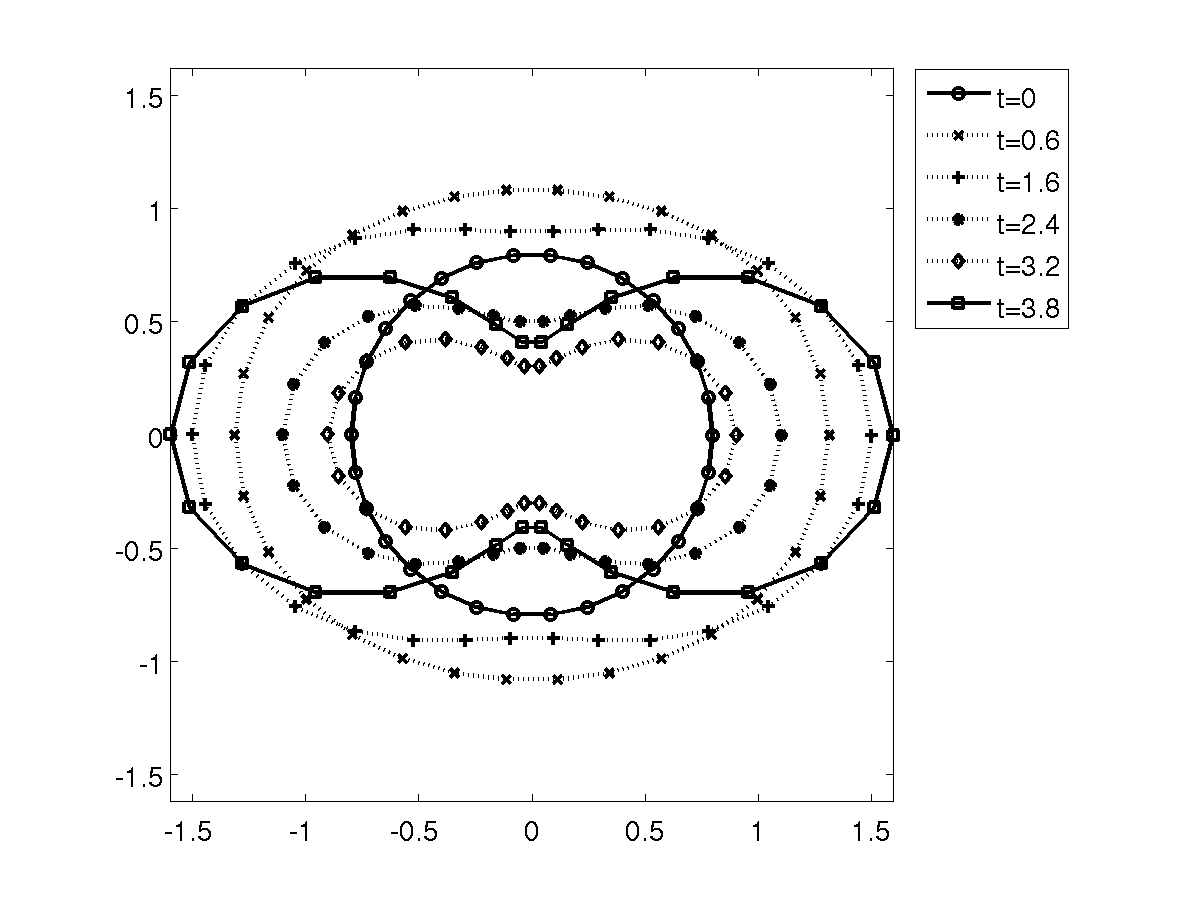
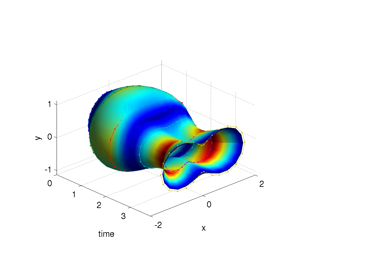
We start with a small family of observation times $0\leq t_{1}<\cdots<t_{M}\leq T$ and for each time, a landmark configuration $x^{D}_{t_{k}}\in\mathbb{R}^{2n}$ defined as a noisy version of regularly sampled curves $c_{k}$. To stay close to some realistic framework where the observation points are sparse, the number $M$ of time points is kept small to $M=5$ (with $t_{5}=3.8$). In these experiments, we focus on the simple Euclidean metric $|x_{t_{k}}^{D}-x_{t_{k}}|^{2}$ in the data term, which is in agreement with our Gaussian noise assumption.

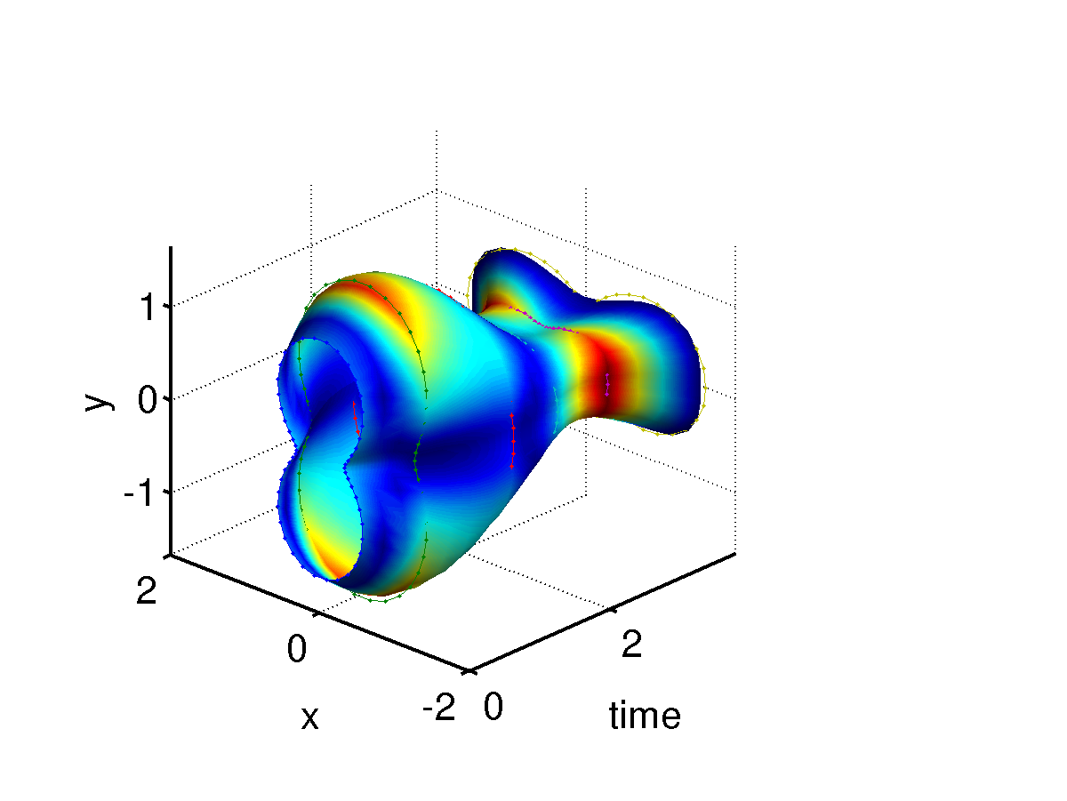
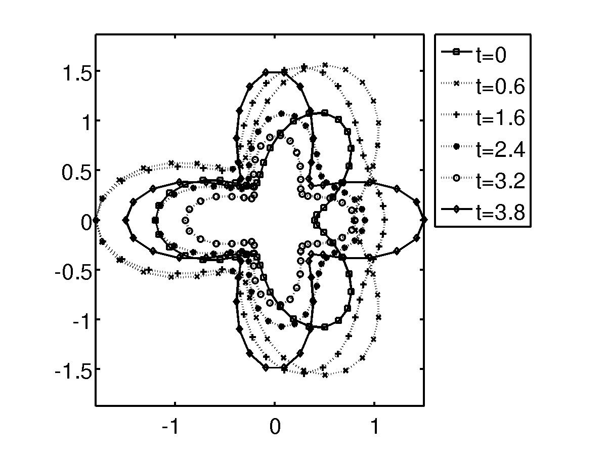
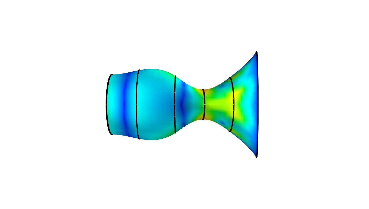
In our first experiment, we consider the evolution of an initial 2D circular shape which somewhat linearly evolves into a pinched ellipsoïdale shape. The shapes are regularity sampled in a consistent way so that the problem of point correspondence between two time points does not need to be consider (see Fig 1). To emphasize the space-time regularity provided by the spline shapes interpolation, we display the result as a surface in the 3D space-time. The first interesting point to note is that the shape spline provides an actual smooth interpolation of the evolution in time between the observation epochs and extends to shape spaces the specific behavior of classical cubic splines. In particular, the shape spline actually joins the observed shapes with very good accuracy despite the fact that we are using here inexact matching.

Figure 2. The figure displays two estimation experiments of shape splines for two different problems. From left to right, the first column displays the sequence of observed shapes, the second and the third column two different viewpoints. The color of any point on the space-time surface is related to the norm of its control variable (with increasing values from deep blue to red)

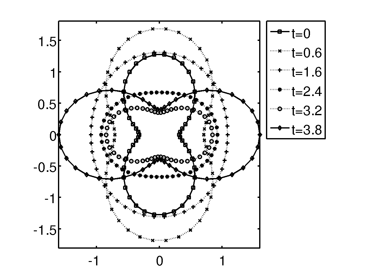
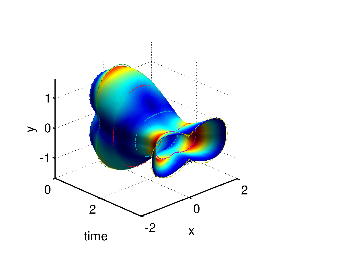
A second important point is that the shape spline comes with the estimation in time of the control variable $u$ which can be interpreted as an external force bending the underlying geodesic. What we see in this example and in the other similar situations, displayed in Fig 2, is that the point-wise values of $u$ give interesting information on the evolution process. More specifically, in every example, the initial and end shape have specific features (numbers of lobes, orientation, etc) and the most active zones are easily interpretable and correspond to transition regions in the shape evolution.

5.1. Robustness to noise

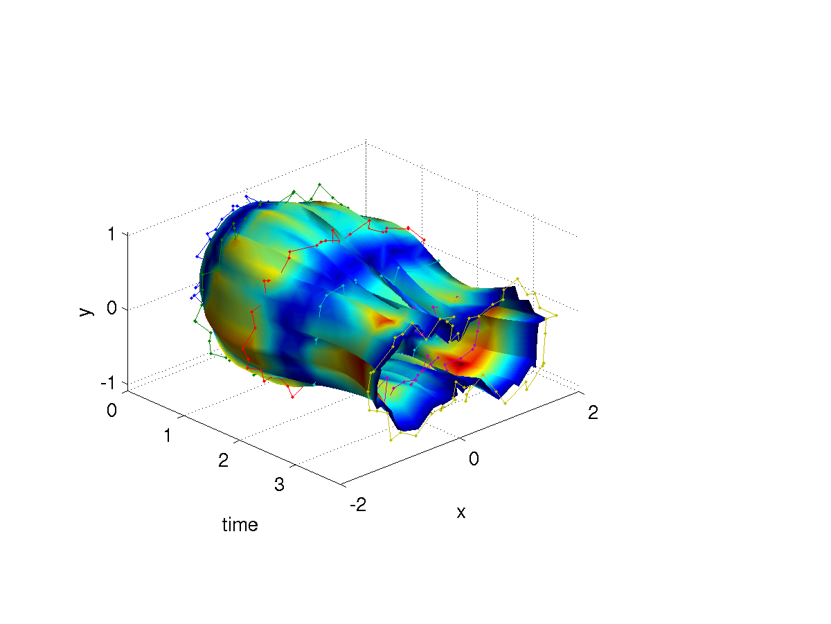
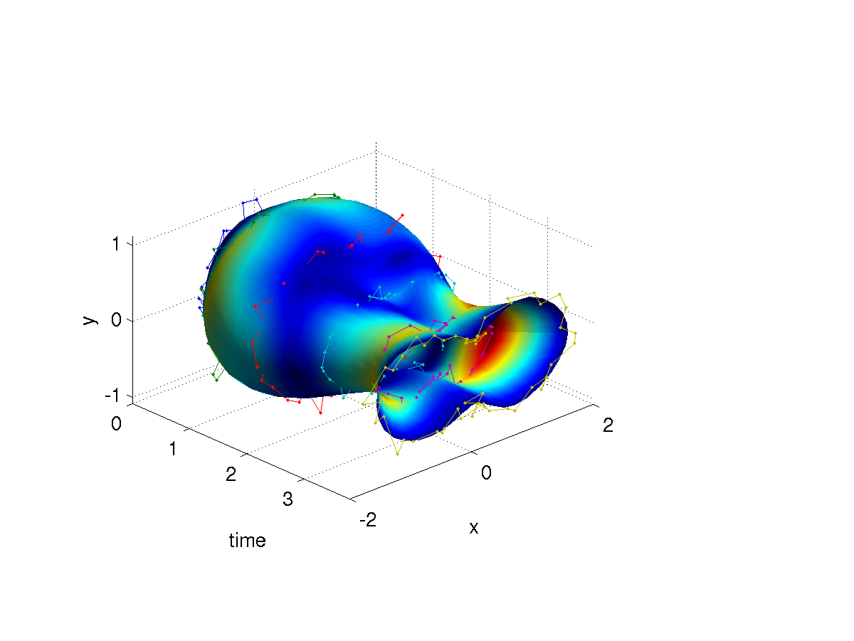
The robustness to noise is a rather important subject from a practical point of view. Indeed, the noise basically degrades the spatial resolution of the measurements so that the evolution through time of a particular point of the evolving curve may be a sharply broken line. The standard spline approach can be quite efficient in filtering this noise if the time sampling frequency is high enough. This is hardly the case in many important situations. However, neighboring points behave coherently through time and offer an interesting source of spatial redundancy.

Figure 3. Robustness to noise. An i.i.d. Gaussian noise with standard deviation $\sigma=0.1$ is added to each measurement point. Shape splines are computed with two different scale parameters, $\lambda=0.001$ on the left, $\lambda=0.6$ on the right.

Much of the large deformation shape space theory involves the integration of spatial redundancy in the comparison between shapes. The shape spline setting, considering shapes as a whole and not as a bag of independent points, keeps this important aspect but adds a time component and considers the problem in the full space-time setting. This robustness to noise is illustrated in Figure 3 where an i.i.d. Gaussian noise with standard deviation $\sigma=0.1$ is added and a series of shape splines are computed under increasing values of the spatial regularity scale parameter $\lambda$ as introduced in (4). For low values of this parameters (with respect to the overall scale of the shapes) the reconstructed evolution is clearly far from any reasonable solution since the spatial redundancy is hardly taken into account. Increasing the value of $\lambda$ to values in accordance to the scale of the object produces a much better reconstruction of the actual shapes at any observation time but also keeps existing time regularity.

5.2. Extrapolation

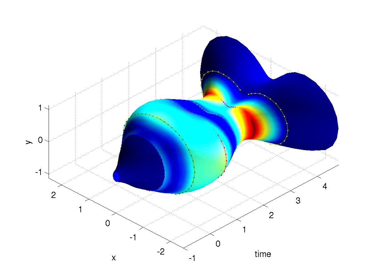
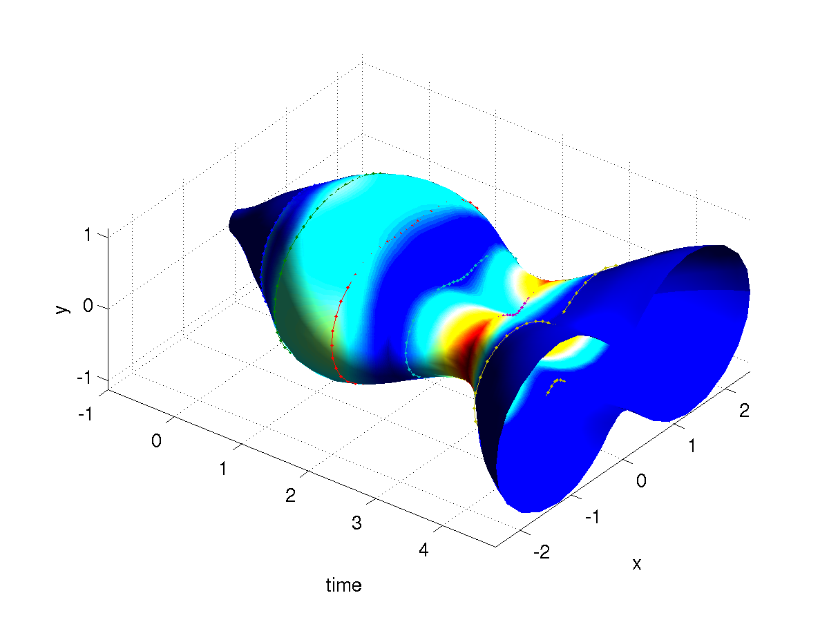
Another distinguished feature of the usual spline setting which is extended in the shape spline setting is the fact that the extrapolation of the data outside the interval of observation is quite straightforward.

Figure 4. Extrapolations. The extrapolation of the evolution at both ends of the observation interval ($\lambda=0.6$, $\sigma=0$).

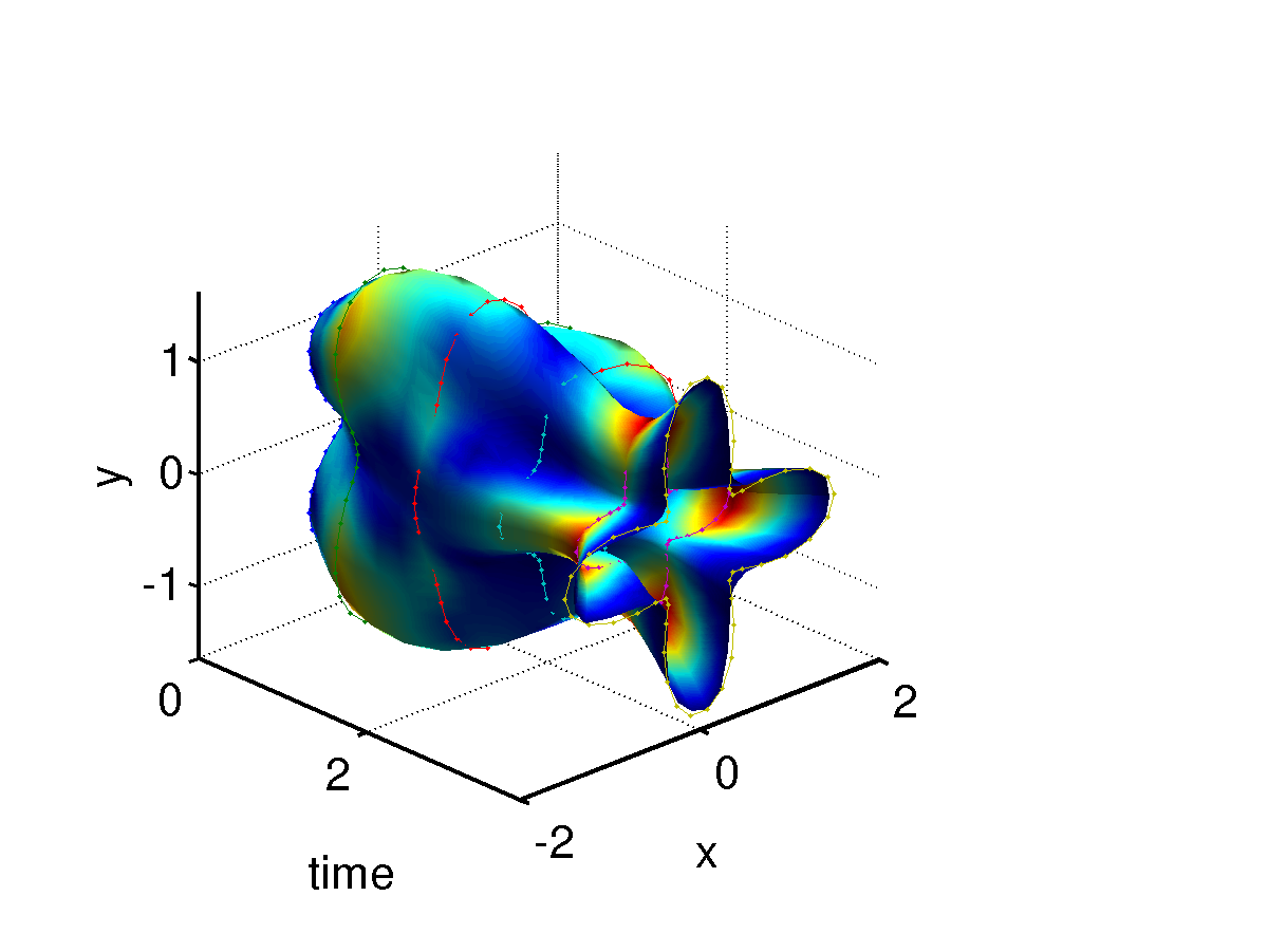
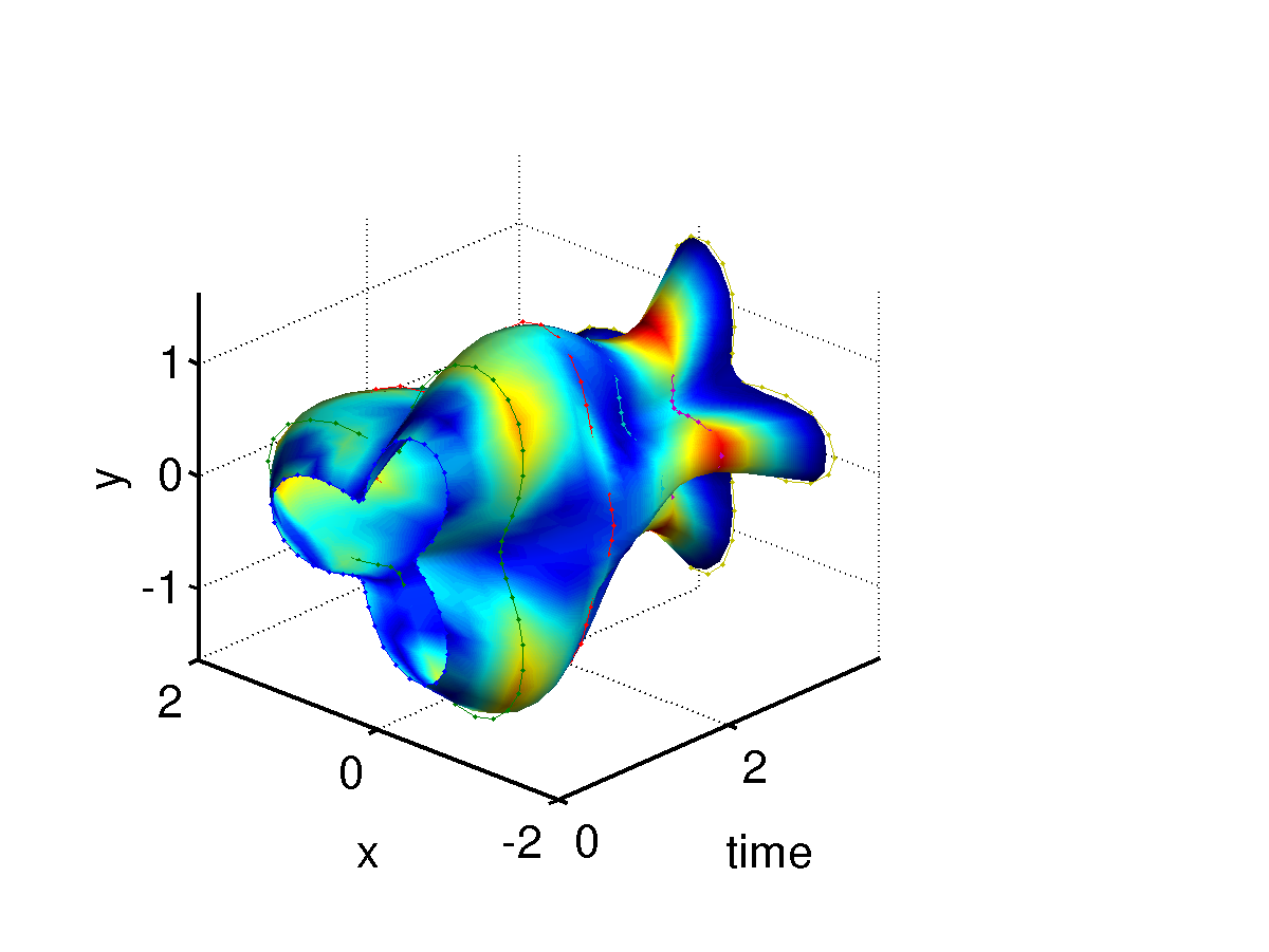
Indeed, outside the limits of the observation interval, the value of the control parameter $u$ is set to zero and the evolution is naturally extended with a geodesic evolution. Moreover, one can check (see Remark 1) that $u$ vanishes at the last observation time so that the previous extension is $C^{0}$ for the control variable $u$ and $C^{1}$ for the shape variable $x$. Note that in the standard growth model described in (12), the evolution is extrapolated by fixing the shape variable to its value at the last observation and this extrapolation is only $C^{0}$. In Figure 4, we display a simple example of extrapolation where the underlying evolution within the observation interval is the same than in Figure 1. The computed extrapolation appears visually quite natural at both ends.

5.3. Comparison with piecewise geodesic evolution

We end this section with a comparison with the piecewise geodesic interpolation scheme [27], derived from (12) for a finite set of observation points as the minimizing solution of

(39) $$J^{x}(v)=\frac{1}{2}\int_{0}^{T}|v_{t}|_{V}^{2}dt+\gamma\sum_{i=1}^{M}|x_{t_{k}}^{D}-x_{t_{k}}|^{2}$$

where as previously stated, $x_{t}=\phi^{v}_{t}(x_{0})$ and $\phi^{v}_{t}$ is the flow of $v\in L^{2}([0,1],V)$.

Figure 5. Comparison with piecewise geodesic evolution. On this example the middle column corresponds to 3 different views of a synthetic shape evolution (here the time axis is vertical in the first two rows and horizontal in the last row). The first column correspond to the piecewise geodesic evolution one can get from (12) and the last one to the shape spline estimation.

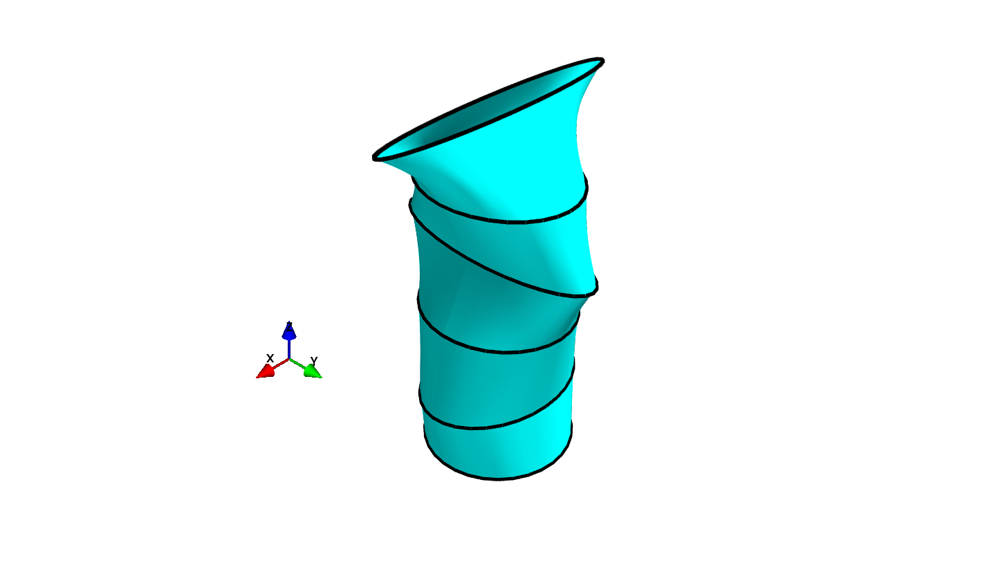
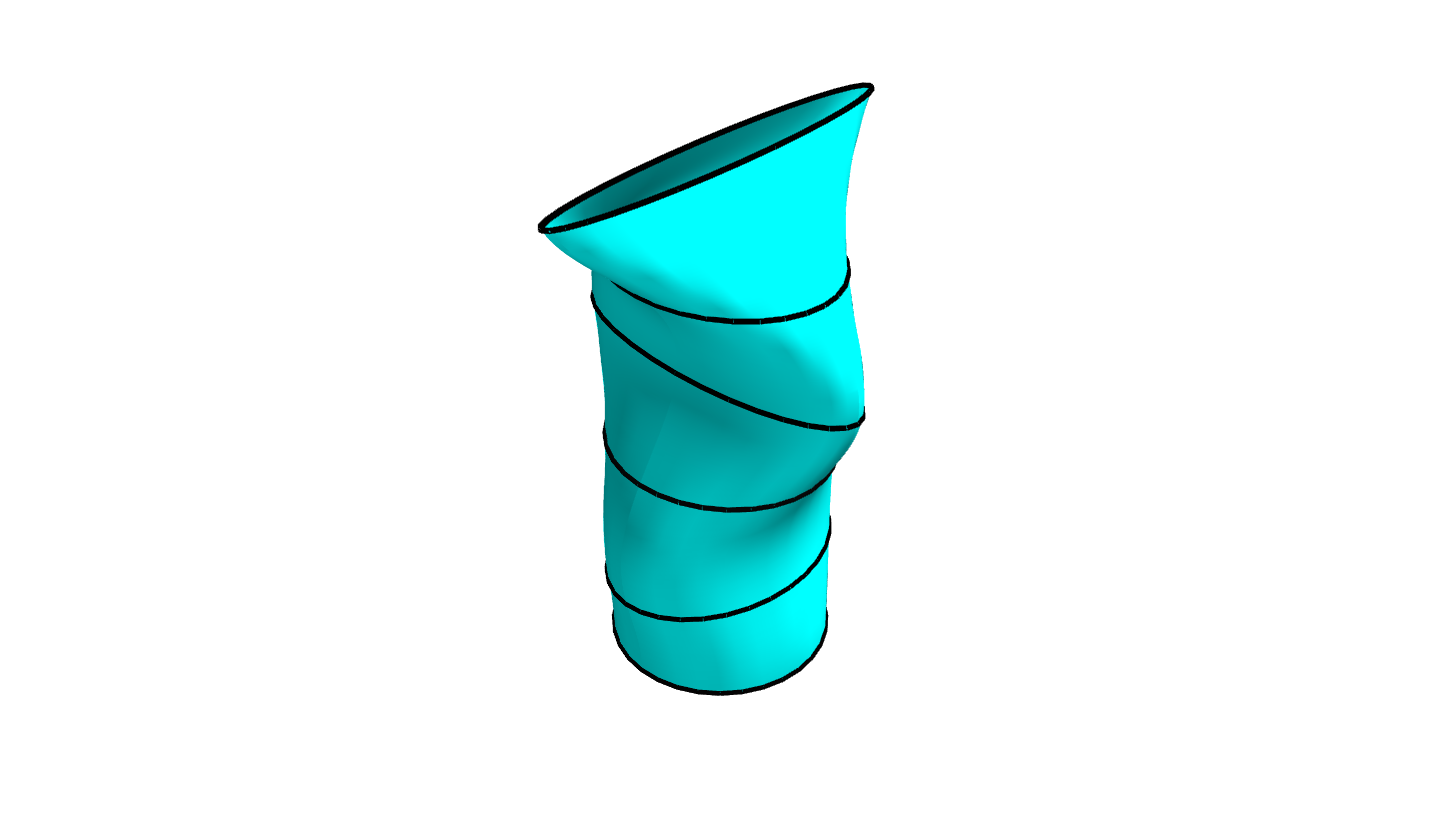
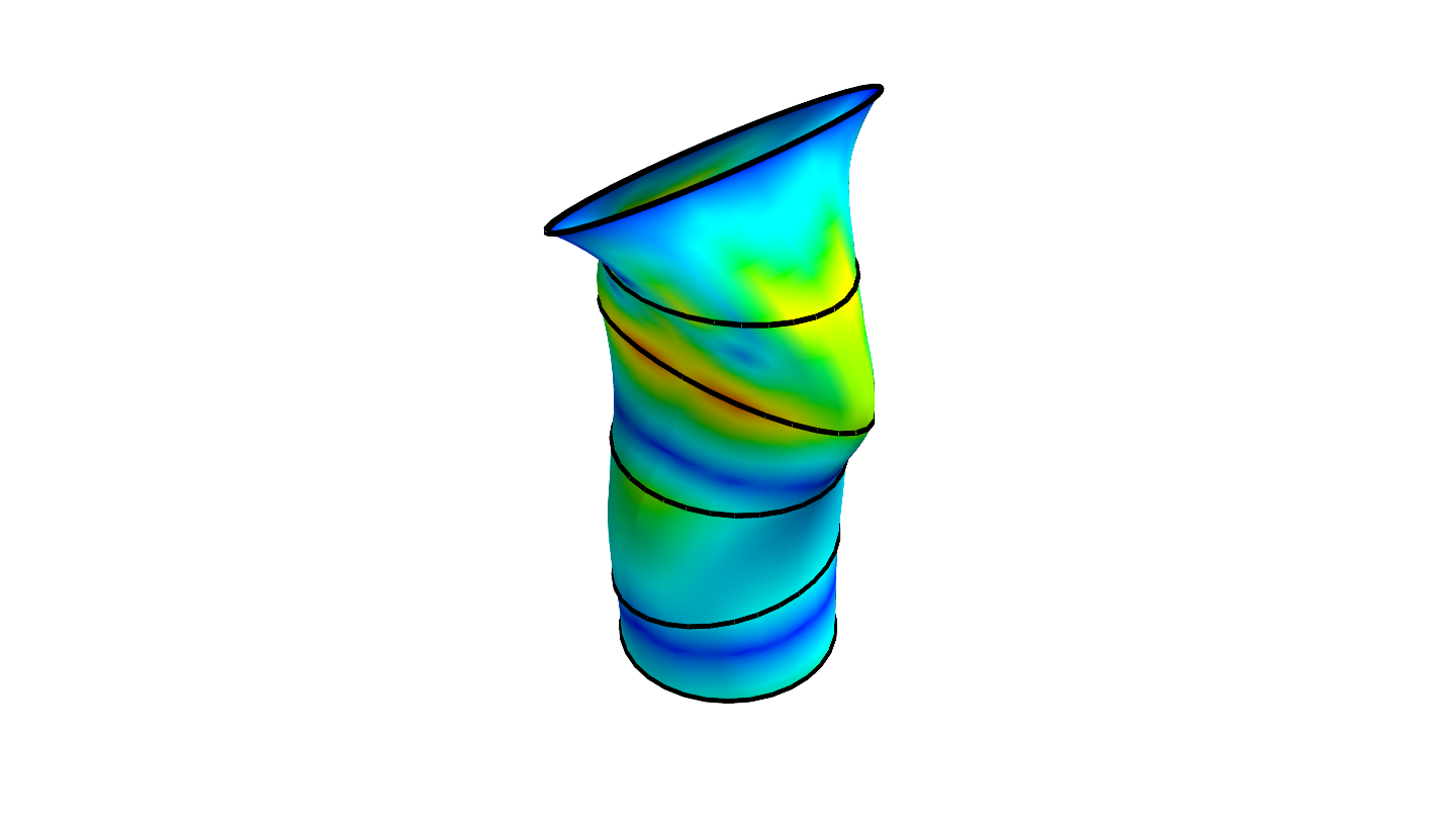
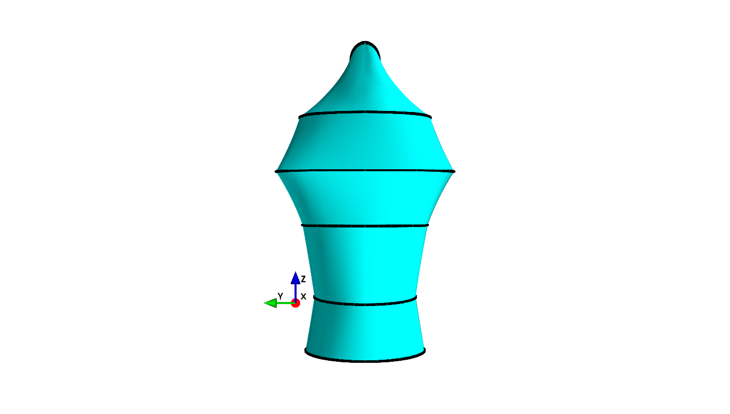
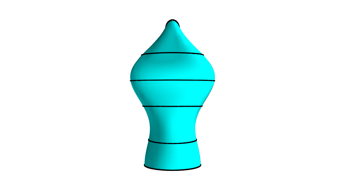
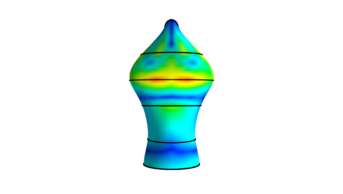
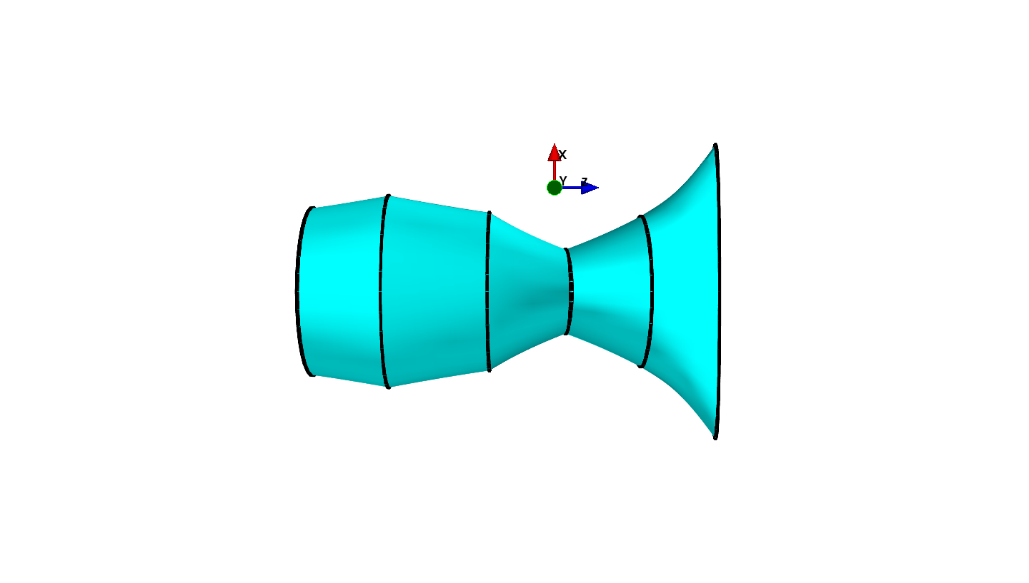
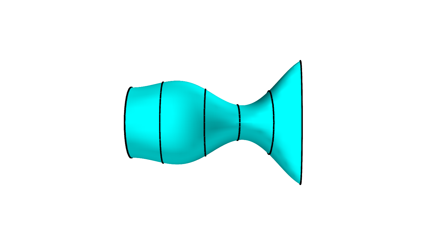
We display an experiment on a synthetic evolution where $t\to x^{D}_{t}$ is given by a simple analytic formula where a circle evolves smoothly into an ellipse by increasing its eccentricity through time combined with a rotation of the principal axis (see three orthogonal views of the synthetic object in the middle column of Fig. 5). We display the estimated evolution in the piecewise geodesic setting given by (39) and with a shape spline in Fig 5. As expected, the piecewise geodesic estimation provides good results but with a loss of regularity at the observation points as in the simpler situation of piecewise linear interpolation in signal processing. The shape spline seems to perform better at the observation points but also to provide a better estimation between observation points.

Figure 6. Comparison of the $L^{2}$ error $E$ (see (40)) between piecewise geodesic and shape spline estimation. The horizontal axis is the number $M$ of observation points and the vertical axis the $L^{2}$ distance in arbitrary units through time between the estimated shape and the actual shape provided by the synthetic evolution. Right panel, log-log plot.

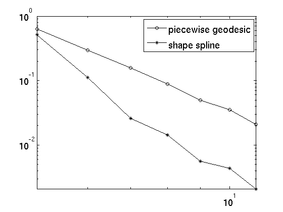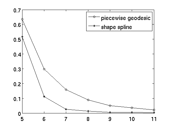
In Fig. 6, we provide a more quantified comparison of the approximation quality between the estimation process by computing the $L^{2}$ error

(40) $$E\doteq\left(\int_{t_{1}}^{t_{M}}|x^{D}_{t}-x_{t}|^{2}dt\right)^{1/2}$$

as a function of the number $M$ of observations. It is quite clear that the convergence is faster with shape spline interpolation than with the piecewise geodesic interpolation (we do not go beyond $11$ observation points since the error is small enough to be approaching other numerical errors in the optimization scheme). The loglog-plot in Fig. 6 seems to indicate a polynomial convergence in $C/M^{\alpha}$ very similar to the classical situation in interpolation theory that ($\alpha=2$ for linear spline and $\alpha=4$ for cubic spline)

6. A stochastic shape spline model

In this section, we study further the first candidate for the second order model (17) of stochastic evolutions of shapes. We prove that the solutions are well defined for all times and present some simulations that highlight some features of this model.

6.1. Non blow-up result

This section is devoted to study the well-posedness of the SDE (17) introduced as our generative growth model in subsection 3.2. The random force is chosen to be an increment of the Brownian motion though we could also have introduced a Levy process in the evolution of the momentum to account for sudden activations of cells. It would turn our growth model into a more realistic one. However, this Brownian perturbation is the first step toward such a model and we will now discuss its feasibility from the mathematical point of view. We will prove that the solutions of the SDE do not blow up in finite time a.s.

The stochastic differential system is:

(41a) $$dp_{t}=-\partial_{x}H_{0}(p_{t},x_{t})\,dt+\varepsilon dB_{t}\,,$$

(41b) $$dx_{t}=\partial_{p}H_{0}(p_{t},x_{t})\,dt\,.$$

Here, $\varepsilon$ is a constant parameter and $B_{t}$ is a Brownian motion on $\mathbb{R}^{dn}$. We will work with the Gaussian kernel but this can be directly extended to other kernels. When $\varepsilon$ is constant, there is no difference studying these stochastic differential equations with the Ito integral or Stratonovich one. However, for a general variance term, we will use the Ito stochastic integral. From the theorem of existence and uniqueness of solution of stochastic differential equation under the linear growth conditions, we can work on the solutions of such equations for a large range of kernels. Yet in our case the Hamiltonian is quadratic, and the classical results for existence and uniqueness of stochastic differential equations only prove that the solution is locally defined. In the deterministic case, this quadratic property could imply existence of a blow-up. To prove that the solutions do not blow up in finite time in the deterministic case ($\varepsilon=0$), we can use the fact that the Hamiltonian of the system is constant in time. By adapting that proof (also closely related to the proposition 2) and controlling the Hamiltonian, we will prove that the solutions are defined for all time.
A first remark we will use is the following, for any $\alpha\in\mathbb{R}^{d}$ and $z\in\mathbb{R}^{d}$,

(42) $$\langle\alpha,K_{V}(z,z)\alpha\rangle_{\mathbb{R}^{d}}\leq C^{2}|\alpha|^{2}_{\mathbb{R}^{d}}\,.$$

Thus, we introduce the stopping times defined as follows: let $M>0$ be a constant and

(43) $$\tau_{M}=\{t\geq 0\,|\,\max(|x_{t}|,|p_{t}|)\geq M\}\,,$$

let also $\tau_{\infty}=\lim_{M\to\infty}\uparrow\tau_{M}$ be the explosion time. Differentiating $H_{0}(p_{t\wedge\tau_{M}},x_{t\wedge\tau_{M}})$ with respect to $t$, we get on $(t<\tau_{M})$:

$$dH_{0}(t)=\partial_{x}H_{0}(p_{t},x_{t})dx_{t}+\partial_{p}H_{0}(p_{t},x_{t})dp_{t}+\sum_{i=1}^{n}\text{tr}(K_{V}(x_{i}(t),x_{i}(t)))\frac{\varepsilon^{2}}{2}dt\,.$$

In the deterministic case the Hamiltonian is constant, whereas here the stochastic perturbation gives

$$\partial_{x}H_{0}(p_{t},x_{t})dx_{t}+\partial_{p}H_{0}(p_{t},x_{t})dp_{t}=\varepsilon\partial_{p}H_{0}(p_{t},x_{t})dB_{t}\,.$$

Thus

$$\int_{0}^{T\wedge\tau_{M}}dH_{0}(t)=\int_{0}^{T\wedge\tau_{M}}\varepsilon\langle\partial_{p}H_{0}(p_{t},x_{t}),dB_{t}\rangle+\int_{0}^{T\wedge\tau_{M}}\sum_{i=1}^{n}\text{tr}(K_{V}(x_{i}(t),x_{i}(t)))\frac{\varepsilon^{2}}{2}dt\,,$$

and

(44) $$E[H_{0}(p_{T\wedge\tau_{M}},x_{T\wedge\tau_{M}})]\leq H_{0}(0)+E(C^{2}\frac{\varepsilon^{2}}{2}dn\,T\wedge\tau_{M})\leq H_{0}(0)+C^{2}\varepsilon^{2}dnT\,.$$

Now, we aim at controlling $x_{t\wedge\tau_{M}}$ using the control on $dx_{t}$ given by $|\partial_{p}H_{0}(p_{t},x_{t})|_{\infty}\leq C\sqrt{H_{0}(p_{t},x_{t})}$:

(45) $$|x_{\tau_{M}\wedge t}|\leq|x_{0}|+\int_{0}^{\tau_{M}\wedge t}CH_{0}(p_{s},x_{s})^{1/2}ds\leq|x_{0}|+\int_{0}^{\tau_{M}\wedge t}CH_{0}(p_{s\wedge\tau_{M}},x_{s\wedge\tau_{M}})^{1/2}ds\\ \leq A_{t}\doteq|x_{0}|+\int_{0}^{\tau_{\infty}\wedge t}CH_{0}(p_{s\wedge\tau_{\infty}},x_{s\wedge\tau_{\infty}})^{1/2}ds\,.$$

However, $0\leq A_{t}$ $P$ a.s. and by monotone convergence theorem (recall that $H_{0}$ is non negative),

$$E(A_{t})=\lim_{M\to\infty}(|x_{0}|+E\left(\int_{0}^{t\wedge\tau_{M}}CH_{0}(p_{s\wedge\tau_{M}},x_{s\wedge\tau_{M}})^{1/2}ds\right).$$

Also,

(46) $$E\left(\int_{0}^{t\wedge\tau_{M}}H_{0}(p_{s\wedge\tau_{M}},x_{s\wedge\tau_{M}})^{1/2}ds\right)\leq E\left(\int_{0}^{t}H_{0}(p_{s\wedge\tau_{M}},x_{s\wedge\tau_{M}})^{1/2}ds\right)\\ \stackrel{{\scriptstyle Fub.}}{{=}}\int_{0}^{t}E\left(H_{0}(p_{s\wedge\tau_{M}},x_{s\wedge\tau_{M}})^{1/2}\right)ds\stackrel{{\scriptstyle Jen.}}{{\leq}}\int_{0}^{t}E\left(H_{0}(p_{s\wedge\tau_{M}},x_{s\wedge\tau_{M}})\right)^{1/2}ds\\ \stackrel{{\scriptstyle CS+~{}(\ref{eq:9.3.1})}}{{\leq}}\sqrt{t}\left(\int_{0}^{t}(H_{0}(0)+C^{2}\varepsilon^{2}dns)\,ds\right)^{1/2}\,.$$

We deduce

$$E(A_{t})\leq|x_{0}|+C\sqrt{t}\left(\int_{0}^{t}(H_{0}(0)+C^{2}\varepsilon^{2}dns)\,ds\right)^{1/2}<\infty\text{ and }A_{t}<\infty\ P\ a.s.$$

and as a consequence

$$\limsup_{M\to\infty}|x_{t\wedge\tau_{M}}|<+\infty\,P\,a.s.$$

We also control the evolution equation of the momentum as follows,

(47) $$|p_{t\wedge\tau_{M}}|\leq\int_{0}^{t\wedge\tau_{M}}|\partial_{x}H_{0}(p_{s},x_{s})|\,ds+|p_{0}+\,\int_{0}^{t\wedge\tau_{M}}\varepsilon dB_{s}\,|\,.$$

Now we use the assumption (3) to control $\partial_{x}H_{0}(p,x)$:

$$|\partial_{x}H_{0}(p,x)|\leq|p||dv(x)|\leq C|p|H_{0}^{1/2}\,.$$

We rewrite inequality (47) and we use Gronwall’s Lemma to get:

$$|p_{t\wedge\tau_{M}}|\leq\int_{0}^{t\wedge\tau_{M}}C|p_{s}|\,H_{0}(p_{s},x_{s})^{1/2}\,ds+|p_{0}+\,\int_{0}^{t\wedge\tau_{M}}\varepsilon dB_{s}\,|\,,$$

$$|p_{t\wedge\tau_{M}}|\leq\left(|p_{0}|+\sup_{u\leq t}|\,\int_{0}^{u\wedge\tau_{M}}\varepsilon dB_{s}\,|\right)e^{\int_{0}^{t\wedge\tau_{M}}CH_{0}(p_{s},x_{s})^{1/2}ds}\,,$$

$$|p_{t\wedge\tau_{M}}|\leq\left(|p_{0}|+\sup_{u\leq t\wedge\tau_{\infty}}|\,\int_{0}^{u}\varepsilon dB_{s}\,|\right)e^{\int_{0}^{t\wedge\tau_{\infty}}CH_{0}(p_{s},x_{s})^{1/2}ds}\,.$$

The first term on the right-hand side $|p_{0}|+\sup_{u\leq t\wedge\tau_{\infty}}|\int_{0}^{u}\varepsilon dB_{s}\,|$ is bounded by $|p_{0}|+\sup_{u\leq t}|\,\int_{0}^{u}\varepsilon dB_{s}\,|<\infty\,P\,a.s.$ and with inequality (46) we have that

$$e^{\int_{0}^{t\wedge\tau_{\infty}}CH_{0}(p_{s},x_{s})^{1/2}ds}<\infty\,P\,a.s.$$

Since on $(\tau_{\infty}\leq t)$ one has

$$\lim_{M\to\infty}\max(|x_{t\wedge\tau_{M}}|,|p_{t\wedge\tau_{M}}|)=\lim_{M\to\infty}|p_{t}|=\infty\,,$$

we deduce $P(\tau_{\infty}\leq t)=0$ and $\tau_{\infty}=+\infty$ almost surely.

We have proved for the case $\varepsilon(p,x)=\varepsilon Id$,

Theorem 4.

Under assumption (3), the solutions of the stochastic differential equation defined by

$$dp_{t} = -\partial_{x}H_{0}(p_{t},x_{t})dt+\varepsilon(p_{t},x_{t})dB_{t}$$

$$dx_{t} = \partial_{p}H_{0}(p_{t},x_{t})dt.$$

are non exploding when $\varepsilon:\mathbb{R}^{nd}\times\mathbb{R}^{nd}\mapsto L(\mathbb{R}^{nd})$ is a Lipschitz and bounded map.

Proof.

To extend the proof to the case when $\varepsilon$ is a Lipschitz and bounded map of $p$ and $x$, we can prove that the preceding inequalities are still valid.

First, with the Lipschitz property of $\varepsilon$ the solutions are still defined locally. The Ito formula is now written as, on $(t<\tau_{M})$

$$dH_{0}(t)=\partial_{x}H_{0}(p_{t},x_{t})dx_{t}+\partial_{p}H_{0}(p_{t},x_{t})dp_{t}+\frac{1}{2}\text{tr}(\varepsilon^{T}(p_{t},x_{t})K_{x_{t}}\varepsilon(p_{t},x_{t}))dt\,.$$

where $K_{x}$ is block matrix defined by $K_{x}\doteq(K_{V}(x_{i},x_{j}))_{1\leq i,j\leq n}$.

We still have the inequality (44) with

$$\text{tr}(\varepsilon^{T}(p_{t},x_{t})K_{x_{t}}\varepsilon(p_{t},x_{t}))\leq(Cnd|\varepsilon|_{\infty})^{2}$$

if $|\varepsilon(p,x)w|^{2}\leq|\varepsilon|_{\infty}^{2}|w|_{\infty}^{2}$ where $|\epsilon|_{\infty}$ denotes the supremum norm. Indeed, if $(e_{i})_{i\in[1,nd]}$ the canonical basis of $\mathbb{R}^{nd}$, denoting $\varepsilon\doteq\varepsilon(x,p)$, we have

$$\text{tr}(\varepsilon^{t}K_{x}\varepsilon)=\sum_{i=1}^{nd}\langle\varepsilon(e_{i}),K_{x}\varepsilon(e_{i})\rangle\leq\lambda^{*}_{K_{x}}\sum_{i=1}^{nd}\langle\varepsilon(e_{i}),\varepsilon(e_{i})\rangle\,,$$

where $\lambda^{*}_{K_{x}}$ is the largest eigenvalue of $K_{x}$. We have $\lambda^{*}_{K_{x}}\leq\text{tr}(K_{x})=\sum_{i=1}^{n}\text{tr}(K_{V}(x_{i},x_{i}))$ and using (42) we get $\text{tr}(K_{V}(x_{i},x_{i}))\leq d\lambda^{*}_{K_{V}(x_{i},x_{i})}\leq dC^{2}$ so that $\lambda^{*}_{K_{x}}\leq C^{2}nd$. Hence,

$$\text{tr}(\varepsilon^{t}K_{x}\varepsilon)\leq C^{2}nd\sum_{i=1}^{nd}|\varepsilon|_{\infty}^{2}\leq(Cnd|\varepsilon|_{\infty})^{2}\,.$$

Thus we get,

$$\int_{0}^{T\wedge\tau_{M}}dH_{0}(t)\leq\int_{0}^{T\wedge\tau_{M}}\langle\partial_{p}H_{0}(p_{t},x_{t}),\varepsilon(p_{t},x_{t})dB_{t}\rangle+\int_{0}^{T\wedge\tau_{M}}\frac{(Cnd|\varepsilon|_{\infty})^{2}}{2}dt\,,$$

$$E[H_{0}(T\wedge\tau_{M})]\leq H_{0}(0)+E(\frac{(Cnd|\varepsilon|_{\infty})^{2}}{2}\,T\wedge\tau_{M})\leq H_{0}(0)+(Cnd|\varepsilon|_{\infty})^{2}\,T\,,$$

and all the remaining inequalities follow easily thanks to the control on $H_{0}$ and the bound on $\varepsilon$. ∎

Once this stochastic model is well-posed on landmark space, the question of its extension to shape spaces naturally arises. It can be proved that this stochastic model does have an extension to the infinite dimensional case: in the case of $L^{2}(\mathbb{R}/\mathbb{Z},\mathbb{R}^{2})$, the natural extension of the Brownian motion on the landmark space is a cylindrical Brownian motion on $L^{2}(\mathbb{R}/\mathbb{Z},\mathbb{R}^{2})$. It may be somewhat surprising to deal with such irregular noise on the momentum variable, we stress the fact that this noise is read by the kernel which strongly regularizes the noise. Though we will not develop it further, it proves that this model has a consistent extension to continuous-shape spaces and could be used to deal with random evolutions of continuous shapes.

6.2. Simulations

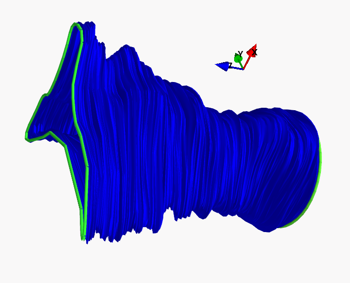
With these simulations we illustrate the interesting features we observed above. First, this model gives realistic perturbations of geodesics contrary to a first order model such as a Kunita flow. A simulation of a Kunita flow is illustrated in figure Fig. 7 where the evolution of $40$ points on the unit circle is represented under a Gaussian kernel of width $0.9$. The time evolution has, as expected, the roughness of a Brownian motion and the space variation is smoother due to the kernel. In comparison, our stochastic model gives smoother evolutions in time as in Fig. 11 and Fig. 11.

Figure 7. A simulation of Kunita flow with $40$ points on the unit circle on the left of the figure. The $z$ axis (blue arrow) represents the time.

Second, our stochastic model is a perturbation of a geodesic evolution and this nice property is illustrated in figures Fig. 9 - 11.

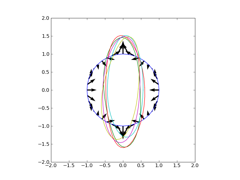
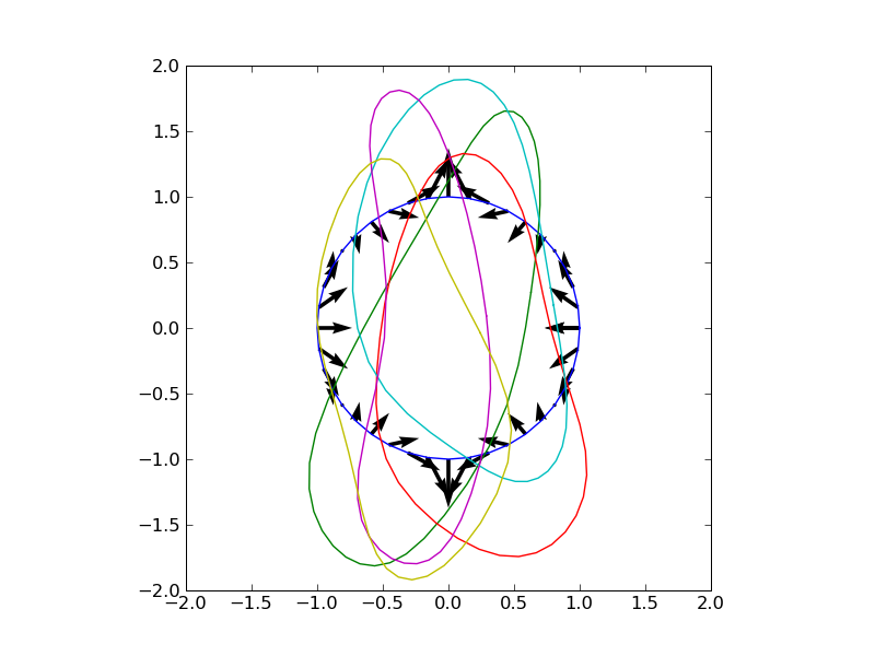
Figure Fig. 9 shows the geodesic evolution of $40$ equidistributed points on the unit circle for a Gaussian kernel of width $1.0$, the target configuration for the landmarks is obtained through a simple affine transformation that gives the final ellipse. On these simulations the color change only represents time. Figures Fig. 9 - 11 represent stochastic perturbations of the previous geodesic; we progressively increase the standard deviation $\epsilon$ of the noise from $\sqrt{n}\epsilon=0.9$ to $1.7$ and finally $\sqrt{n}\epsilon=3.5$ (the noise is rescaled w.r.t. the number of landmarks to converge to a well defined SPDE at the limit (see [34])). Each of these three figures represents one Monte-Carlo simulation of the stochastic model with a simple Euler scheme.

Figure 8. Geodesic evolution - White unit circle as initial shape.

Figure 9. White noise perturbation of the geodesic (same initial momentum $p_{0}$), $\sqrt{n}\epsilon=0.9$

Figure 10. Increasing the variance of the noise, $\sqrt{n}\epsilon=1.7$

Figure 11. Increasing the variance of the noise, $\sqrt{n}\epsilon=3.5$

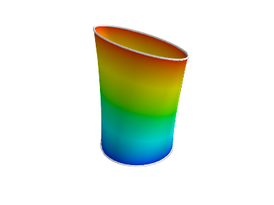
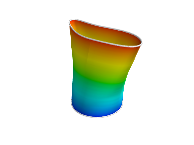
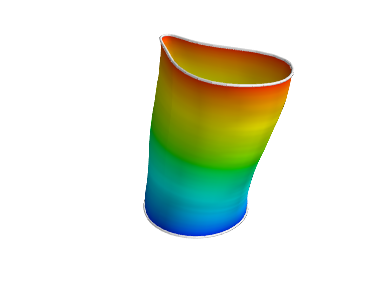
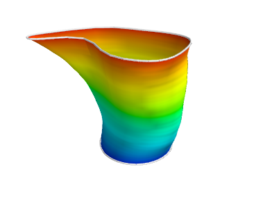
The simulations in figures Fig. 12 show the position at time $1$ of the $40$ points for $5$ Monte-Carlo simulations. On the two figures we plotted the initial momentum $p_{0}$ (attached to the $40$ points) associated with the geodesic from the initial circle to the target ellipse. As this model was designed to produce random shape evolutions, it can also be used as a generative engine to produce random shapes. Increasing the noise also increases the expectation of the energy of the system since the Ito formula applied on the Hamiltonian in subsection 6.1 shows a linear growth in time of $H_{0}$ proportional to $\varepsilon$. This can be guessed when comparing the two displayed cases in Fig. 12 since in the second one the noise is $4$ times bigger. For any statistical estimation of the model parameters, this property should be somehow taken into account.

Figure 12. Effects of the standard deviation $\epsilon$ of the noise : $5$ simulations of random deformations of the unit circle. The initial momentum $p_{0}$ is fixed, the kernel width $\lambda=1$ (see (4)). Left-hand side : $\sqrt{n}\epsilon=0.25$ ; right-hand side : $\sqrt{n}\epsilon=1$.

An important feature of this model is that the noise is "read" by the kernel. We show in Fig. 13 simulations of the model for a null initial momentum on the same initial shape and we decrease the width of the Gaussian kernel from $3$ to $0.3$. The standard deviation of the noise is constant set to $\sqrt{n}\epsilon=1.0$.

Figure 13. Effects of the width of the Gaussian kernel. Left-hand side :$\lambda=0.3$ ; right-hand side : $\lambda=3.0$.

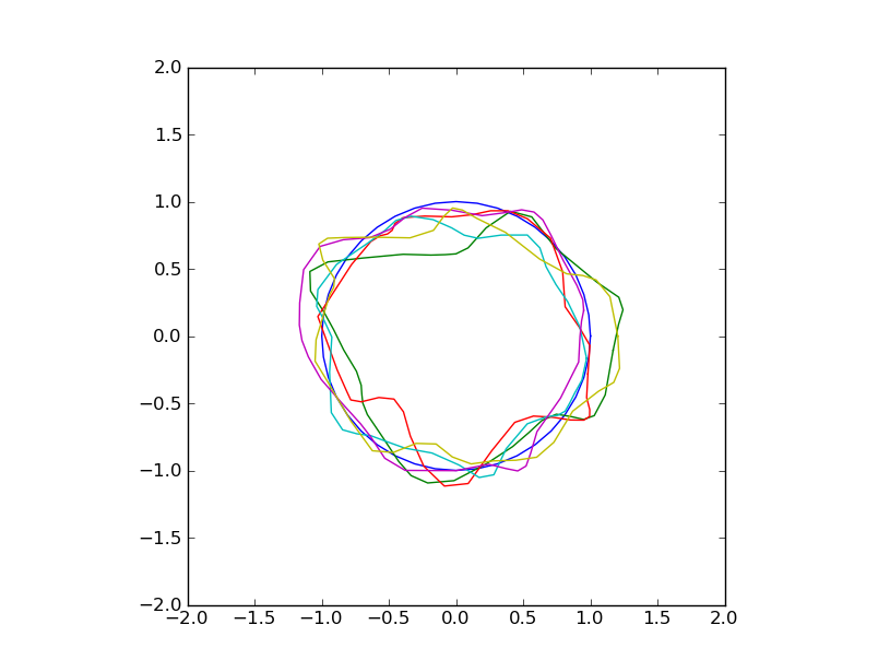
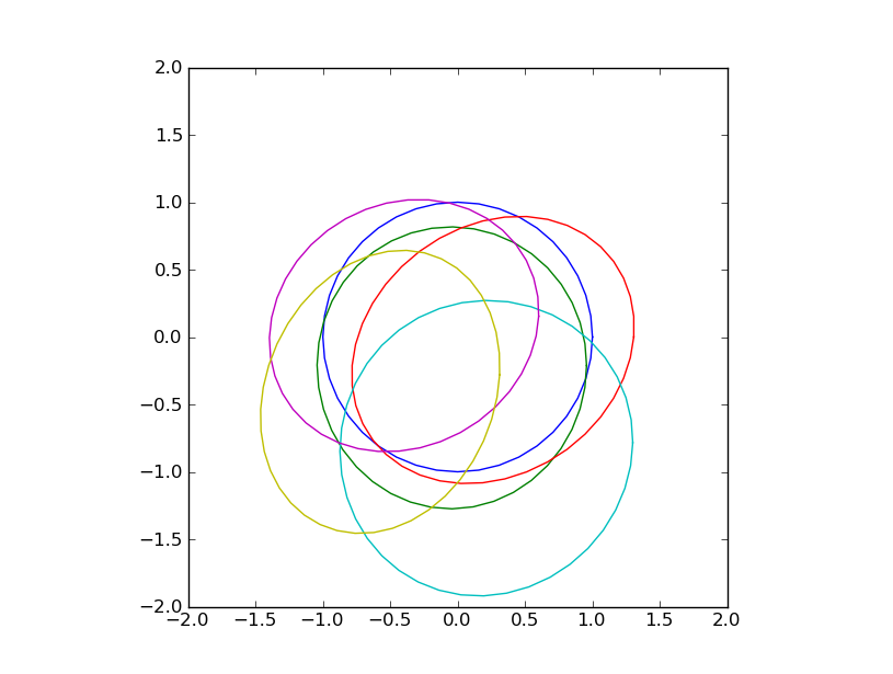
These last simulations show the importance of the choice of the kernel and as a by-product the choice of the operator $\varepsilon$ in front of the noise will be also important. Now we can formulate a stochastic model for evolutions of shape that would be closer to realistic evolutions:

(48) $$\begin{cases}dp_{t}=-\partial_{q}H_{0}(p_{t},q_{t})+u_{t}+\varepsilon dB_{t}\\ dq_{t}=\partial_{p}H_{0}(p_{t},q_{t})\,,\end{cases}$$

where $u_{t}$ is of bounded variations. At this point, we underline that the model parameterization is completely open and it should be tightly related to consistent statistical estimations.

7. Shape splines on homogeneous space

In this section we provide a more formal and geometrical picture of what could be an extension of the shape spline to the previously mentioned important cases. For this, we need to introduce some of the standard vocabulary of geometrical mechanics as developed in [25]. We will try as much as possible to avoid the conceptual burden of the intrinsic differential and symplectic geometry through the extensive use of local coordinates. Readers looking for a more intrinsic formulation could refer to [25].

7.1. Geometrical setting

The proposed framework for shape spline is given by three ingredients: a group $G$ of transformations, a Riemannian manifold $Q$ and a left action of $G$ on $Q$ denoted $(g,q)\to L_{q}(g)\doteq g\cdot q$. We will assume also that for any $q\in Q$, $g\to g\cdot q$ is a surjective submersion (i.e. the differential of $L_{q}$ has full rank everywhere).

7.1.1. Local coordinates

Basically $G$ will be a (finite dimensional) Lie group with Lie algebra $\mathfrak{G}$ on which we consider a right invariant metric given by a dot product on $\mathfrak{G}$. The infinite dimensional setting where $G$ is a group of diffeomorphisms is more involved and requires more analytical work as in [33]. This is clearly the target setting we have in mind but we want in this paper to stay away from any complicated analytical developments. To keep the focus on the global picture, we will assume implicitly that we work in a finite dimensional setting for which the existence of all the introduced objects is straightforward.

Denoting $q=(q^{1},\cdots,q^{n})$ local coordinates on $Q$ and since $(dq^{1},\cdots,dq^{n})$ is a basis of $T_{q}^{*}Q$, we can write any $\alpha\in T^{*}_{q}Q$ as $\alpha=\sum p_{i}dq^{i}$ so that $(q^{1},\cdots,q^{n},p_{1},\cdots,p_{n})$ are local coordinates on the cotangent bundle $T^{*}Q$. Given $q=(q^{1},\cdots,q^{n})$, we will denote $p=(p_{1},\cdots,p_{n})$ a generic element of $T_{q}^{*}Q$ and $m=(q,p)$ a generic element of $T^{*}Q$ as we did previously in the flat case of landmarks.

7.1.2. Infinitesimal actions and cotangent lift

The first thing we need is to extend the action of $G$ on $Q$ to an action of $G$ on the cotangent bundle $T^{*}Q$. Note that the differentiation in $g$ of $g\to q\cdot q$ at $g=\text{Id}_{G}$ yields an infinitesimal action $(\xi,q)\to\xi\cdot q$ for $\xi\in\mathfrak{G}$. Differentiation in $q$ yields the action $(g,\delta q)\to g\cdot\delta q\in T_{g\cdot q}Q$ for $\delta q\in T_{q}Q$ and by duality the action $(g,p)\to g\cdot p\in T_{g\cdot q}^{*}Q$ for $p\in T_{q}^{*}Q$, uniquely defined through the equality

(49) $$(g\cdot p|g\cdot\delta q)\doteq(p|\delta q)\,.$$

We denote

(50) $$(g,m)\to m\cdot g\doteq(g\cdot q,g\cdot p)$$

for $m=(q,p)\in T^{*}Q$ the induced action on $T^{*}Q$.

In summary, the initial action $g\to g\cdot q$ on $Q$ is naturally lifted to an action $g\to g\cdot m$ on the cotangent space $T^{*}Q$ (usually called cotangent lift [25]). Differentiating the action $(g,m)\to g\cdot m$ on the cotangent space $T^{*}Q$ at $g=\mathrm{Id}_{G}$, we get the infinitesimal action on $T^{*}Q$, which is defined in local coordinates by $\xi\cdot m=(\xi\cdot q,\xi\cdot p)$ where

(51) $$(\xi\cdot p|\delta q)+(p|\xi\cdot\delta q)=0$$

as obtained by differentiation of the conservation equation (49).

7.2. Euler-Poincaré equation

The initial matching problem between shapes in $Q$ is defined as the solution of the optimal control problem with fixed boundary

$$\left|\begin{array}[h]{l}\min_{\xi_{t}}\frac{1}{2}\int_{0}^{1}(L\xi_{t},\xi_{t})dt\\ \text{subject to}\\ \dot{q}_{t}=\xi_{t}\cdot q_{t},\ q_{0}=q_{\text{init}},\ q_{1}=q_{\text{targ}}\end{array}\right.$$

where $L:\mathfrak{G}^{*}\to\mathfrak{G}$ is the isometry between $\mathfrak{G}$ and its dual induced by the metric on $\mathfrak{G}$.

The Hamiltonian associated to the classical matching problem is given in local coordinates by $H(q,p,\xi)=(p|\xi\cdot q)-\frac{1}{2}(L\xi|\xi)$ with reduced form

$$H(q,p)\doteq\frac{1}{2}\big{(}KJ(q,p)\,|\,J(q,p)\big{)}$$

where $J(q,p)\in\mathfrak{G}^{*}$ is uniquely defined by

(52) $$(J(q,p)|\xi)=(p|\xi\cdot q)$$

for any $\xi\in\mathfrak{G}$ (usually called the momentum map). To obtain the Hamiltonian evolution, we need to compute the variation of $\delta J$ as a function of the variation $\delta q$ and $\delta p$ in $q$ and $p$. Introducing in local coordinates the so-called symplectic matrix

$$\mathbb{J}\doteq\left(\begin{array}[h]{cc}0&\text{Id}_{n}\\ -\text{Id}_{n}&0\end{array}\right)$$

one checks easily that $(\delta J|\xi)=(p|\xi\cdot\delta q)+(\delta p|\xi\cdot q)$ so that using (51) we get

(53) $$(\delta J|\xi)=-(\xi\cdot p|\delta q)+(\delta p|\xi\cdot q)=-(\mathbb{J}(\xi\cdot m)|\delta m)$$

and $dH=-\mathbb{J}(KJ\cdot m)$. Since the associated Hamiltonian evolution equation are given by $\dot{m}=\mathbb{J}dH$ we get

(54) $$\dot{m}=Kj\cdot m\text{ with }j=J(q,p)$$

or equivalently

(55) $$\dot{q}=\xi\cdot q\text{ and }\dot{p}=\xi\cdot p\text{ with }\xi=KJ(q,p)\,.$$

This extremely simple expression of $\dot{m}$ in term of the momentum map and the infinitesimal action on the cotangent space reveals part of the nice geometrical structure underlying the evolution. In this setting, it is interesting to consider the time evolution of the pair $(q,j)$ instead of the pair $(q,p)$ since $j$ follows an autonomous equation. Indeed, from (51) and (55), we get that for any $\zeta\in\mathfrak{G}$ we have $(\frac{dj}{dt}\ |\ \zeta)=(\xi_{t}\cdot p\ |\ \zeta\cdot q)+(p\ |\ \zeta.(\xi_{t}\cdot q))=(p\ |\ \zeta.(\xi_{t}\cdot q)-\xi_{t}\cdot(\zeta\cdot q))=-(p\ |\ \mathrm{ad}_{\xi_{t}}(\zeta)\cdot q)=-(j\ |\ \mathrm{ad}_{\xi_{t}}(\zeta))$ where $\mathrm{ad}_{\xi}(\zeta)=[\xi,\zeta]$ is the adjoint representation of the Lie algebra $\mathfrak{G}$ so that we get

$$\frac{dj}{dt}+\mathrm{ad}^{*}_{Kj}j=0\,.$$

This equation, called the Euler-Poincaré equation plays a central role in geometric mechanics and more recently in the large deformation methods in shape analysis and computational anatomy [16, 25].

Now consider the perturbed dynamic $\dot{p}=Kj(m).p+u$ with $u\in T_{q}^{*}Q$ or equivalently

$$\frac{dj}{dt}+\mathrm{ad}^{*}_{Kj}j=h$$

where $h\doteq J(q,u)$ and the associated optimal control problem for the state variables $(q,j)\in Q\times\mathfrak{G}^{*}$ and the cost $\frac{1}{2}|u|^{2}_{q,*}$. The norm $|u|_{q,*}$ we consider here is the dual norm induced on $T_{q}^{*}Q$ by the metric on $T_{q}Q$. Let $\mathcal{K}_{q}:T_{q}^{*}Q\to T_{q}Q$ be the isometry such that $(u\ |\ \mathcal{K}_{q}u)=|u|_{q,*}^{2}$. The Hamiltonian associated to our new control problem for the costate variable $(p_{q},\zeta)\in T_{q}^{*}Q\times\mathfrak{G}$ is given by

(56) $$\mathcal{H}(q,j,p_{q},\zeta,u)=(p_{q}\ |\ Kj\cdot q)+(-\text{ad}_{Kj}^{*}j+h\ |\ \zeta)-\frac{1}{2}(\mathcal{K}_{q}u\ |\ u)\,.$$

To compute its reduced form let us note that from (51), we get $\frac{\partial}{\partial u}(h\ |\ \zeta)=\zeta\cdot q$. Hence $\frac{\partial}{\partial u}\mathcal{H}=0$ implies $\mathcal{K}_{q}u=\zeta\cdot q$ giving the reduced Hamiltonian

(57) $$\mathcal{H}(q,j,p_{q},\zeta) = (p_{q}\ |\ Kj\cdot q)+(-\text{ad}_{Kj}^{*}j\ |\ \zeta)+\frac{1}{2}|\zeta\cdot q|^{2}_{q}$$

(58) $$= (J(q,p_{q})\ |\ Kj)+(j\ |\ \text{ad}_{\zeta}(Kj))+\frac{1}{2}|\zeta\cdot q|^{2}_{q}\,,$$

where $|\ |_{q}$ denote the norm on $T_{q}Q$ given by the Riemmanian metric on $Q$. The associated Hamiltonian evolution is derived quite easily:

(59) $$\left\{\begin{array}[h]{l}\xi=Kj\\ \frac{dq}{dt}=\xi\cdot q\\ \frac{dp_{q}}{dt}-\xi.p_{q}=-\frac{\partial}{\partial q}(\frac{1}{2}|\zeta\cdot q|^{2}_{q})\\ \frac{dj}{dt}+\text{ad}_{\xi}^{*}(j)=\frac{\partial}{\partial\zeta}(\frac{1}{2}|\zeta\cdot q|^{2}_{q})\\ \frac{d\zeta}{dt}+\text{ad}_{\zeta}(\xi)+K\text{ad}_{\zeta}^{*}(j)+KJ(q,p_{q})=0\end{array}\right.$$

Here again, the derivation should be considered at a formal level or in a smooth finite dimensional setting since existence results are beyond the scope of this paper.

8. Conclusion

In this paper, we present new tools for shape evolution analysis or growth analysis in computational anatomy through the introduction of second order evolutions. Shape splines seem to overcome some of the limitations of the previous first order schemes and with their stochastic counterpart can provide the backbone of new statistical time regression tools. From various perspectives, shape splines offer new interesting mathematical and practical challenges: extensions to the infinite dimensional case of continuous shapes and to images, development of efficient and scalable numerical schemes to solve the spline estimation problem, integration of time realignment as developed in [9], derivation of more complex stochastic engines beyond the white-noise situation presented here and development of consistent statistical schemes in the spirit of [3]. The solutions to some of these problems appear well within reach.

In this paper we preferred to stick to the finite dimensional setting in order to focus on the general picture and avoid more difficult analysis, the more technically involved infinite dimensional situation has been partially explored in the stochastic case in [34]. Acknowledgments. The authors would like to thank Darryl D. Holm and Colin J. Cotter for a fruitful discussion about introducing noise on the momentum variable which was the starting point of the stochastic model presented here.

9. Appendix

9.1. Link with cubic splines

We recall that on a Riemannian manifold $(M,g_{M})$, a cubic spline between $(x_{0},v_{0})$ and $(x_{1},v_{1})$ is a $C^{2}$ curve $c:[0,1]\to M$ that minimizes

(60) $$\mathcal{I}(c)=\frac{1}{2}\int_{0}^{1}g_{M}(\nabla_{\dot{c}}\dot{c},\nabla_{\dot{c}}\dot{c})\,dt\,.$$

The Euler-Lagrange equation for this functional is the following (see [29, 11])

(61) $$\nabla^{3}_{t}\dot{c}+R(\nabla_{t}\dot{c},\dot{c})\dot{c}=0\,.$$

Let $c:I\to M$ a smooth path, then the covariant derivative is given in coordinates by

$$\nabla_{\dot{c}}\dot{c}=[\ddot{c}_{i}+\sum_{k,l}\dot{c}_{k}\Gamma_{k,l}^{i}(c)\dot{c}_{l}]_{i\in[1,r]},$$

and we observe that the second member of the right hand side only depends on $(\dot{c},c)$. We compare this expression with the Hamiltonian equations (here $M=\mathcal{L}$):

(62) $$\ddot{c}=\frac{d}{dt}k(c,c)p=[\partial_{1}k(c,c)](\dot{c})p+k(c,c)\dot{p}\,,$$

(63) $$\ddot{c}=[\partial_{1}k(c,c)](k(c,c)^{-1}p)p-k(c,c)\partial_{x}H+k(c,c)u\,,$$

where for any $x,y\in\mathbb{R}^{nd}$, $k(x,y)$ denotes the block matrix defined by

$$k(x,y)\doteq(K_{V}(x_{i},y_{j}))_{1\leq i,j\leq n}\,.$$

Now the geodesic equations are given by

$$\ddot{c}_{i}+\sum_{k,l}\dot{c}_{k}\Gamma_{k,l}^{i}(c)\dot{c}_{l}=0\;\text{for}\,i\in[1,r]\,,$$

where $\Gamma_{k,l}^{i}=g_{\mathcal{L}}(\nabla_{\partial_{i}}\partial_{j},\partial_{k})$ are the Christoffel symbols in the chosen coordinates.

However, if $u=0$ we obtain the geodesic equations in the Hamiltonian form. Then we can identify

$$-[\sum_{k,l}\dot{c}_{k}\Gamma_{k,l}^{i}(c)\dot{c}_{l}]_{i\in[1,r]}=[\partial_{1}k(c,c)](k(c,c)^{-1}p)p-k(c,c)\partial_{x}H\,,$$

which gives

$$\nabla_{\dot{c}}\dot{c}=k(c,c)u\,.$$

Now we have

$$g_{\mathcal{L}}(\nabla_{\dot{c}}\dot{c},\nabla_{\dot{c}}\dot{c})=g_{\mathcal{L}}(k(c,c)u,k(c,c)u)=\langle u,k(c,c)u\rangle\,,$$

which proves the desired result.

9.2. Proof of Proposition 1

Let us denote $\partial_{12}K_{W}(z_{1},z_{2})\doteq\frac{\partial^{2}K_{W}}{\partial z_{1}\partial z_{2}}(z_{1},z_{2})$ for any $z_{1},z_{2}\in\mathbb{R}^{d}$ and $\Delta_{z,h,\epsilon}\doteq\frac{1}{\epsilon}(\delta_{z+\epsilon h}-\delta_{z})$ for any $z,h\in\mathbb{R}^{d}$ and $\epsilon>0$. Let us recall that for any $z_{1},z_{2}\in\mathbb{R}^{d}$

(64) $$\langle\delta_{z_{1}},\delta_{z_{2}}\rangle_{W^{*}}=K_{W}(z_{1},z_{2})\,.$$

First, we start with the proof that $\Delta_{z,h,\epsilon}$ converges in $W^{*}$ when $\epsilon\to 0$. Indeed we get from (64) that

(65) $$\langle\Delta_{z_{1},h_{1},\epsilon_{1}},\Delta_{z_{2},h_{2},\epsilon_{2}}\rangle_{W^{*}} = \int_{0}^{1}\int_{0}^{1}\partial_{12}K_{W}(z_{1}+s\epsilon_{1}h_{1},z_{2}+t\epsilon_{2}h_{2})\cdot h_{1}\otimes h_{2}\,dsdt$$

(66) $$= \partial_{12}K_{W}(z_{1},z_{2})\cdot h_{1}\otimes h_{2}+o((|\epsilon_{1}h_{1}|+|\epsilon_{2}h_{2}|)|h_{1}||h_{2}|)\,,$$

so that $|\Delta_{z,h,\epsilon}-\Delta_{z,h,\epsilon^{\prime}}|^{2}_{W^{*}}=o(|\epsilon|+|\epsilon^{\prime}|)$. Since $W^{*}$ is complete, $\Delta_{z,h,\epsilon}$ converges in $W^{*}$ to a limit point denoted $\delta^{\prime}_{z,h}$ such that $\langle\delta^{\prime}_{z_{1},h_{1}},\delta^{\prime}_{z_{2},h_{2}}\rangle_{W^{*}}=\lim\langle\Delta_{z_{1},h_{1},\epsilon},\Delta_{z_{2},h_{2},\epsilon}\rangle_{W^{2}}=\partial_{12}K_{W}(z_{1},z_{2})\cdot h_{1}\otimes h_{2}$. In particular $h\to\delta^{\prime}_{z,h}$ is a continuous linear mapping from $\mathbb{R}^{nd}$ to $W^{*}$.

Now, we get from (65)

$$|\delta_{z,h}-(\delta_{z}+\delta^{\prime}_{z,h})|^{2}_{W^{*}}=o(|h|^{3})$$

so that $\psi$ is differentiable at any location $x\in\mathbb{R}^{nd}$ with differential $\psi^{\prime}(x)$ given by

$$\psi^{\prime}(x)\Delta x\doteq\frac{1}{n}\sum_{i=1}^{n}\delta^{\prime}_{x_{i},\Delta x_{i}}\,.$$

Thus, using again (65), we get $\langle\psi^{\prime}(x)\Delta x,\psi^{\prime}(x)\Delta x\rangle_{W^{*}}=\frac{1}{n^{2}}\sum_{i,j=1}^{n}\partial_{12}K(x_{i},x_{j})\cdot\Delta x_{i}\otimes\Delta x_{j}$ which proves Proposition 1.

References

- [1] A. A. Agrachev and Y. L. Sachkov. Control theory from the geometric viewpoint, volume 87 of Encyclopaedia of Mathematical Sciences. Springer-Verlag, Berlin, 2004. , Control Theory and Optimization, II.
- [2] J. Ahlberg, E. Nilson, and J. Walsh. The theory of splines and their applications. Mathematics in Science and Engineering, 38, 1967.
- [3] S. Allassonnière, Y. Amit, and A. Trouvé. Towards a coherent statistical framework for dense deformable template estimation. J. R. Statist. Soc. B, 69(1):3–29, 2007.
- [4] S. Allassonniere, A. Trouv , and L. Younes. Geodesic shooting and diffeomorphic matching via textured meshes. In EMMCVPR05, pages 365–381, 2005.
- [5] M. Camarinha, F. S. Leite, and P.Crouch. Splines of class on non-euclidean spaces. IMA Journal of Mathematical Control & Information, 12:399–410, 1995.
- [6] P. Crouch and F. S. Leite. The dynamic interpolation problem: On Riemannian manifold, Lie groups and symmetric spaces. Journal of dynamical & Control Systems, 1:177–202, 1995.
- [7] B. Davis, P. Fletcher, E. Bullitt, and S. Joshi. Population shape regression from random design data. In Computer Vision, 2007. ICCV 2007. IEEE 11th International Conference on, pages 1–7, Oct. 2007.
- [8] I. L. Dryden and K. V. Mardia. Statistical Shape Analysis. 1998.
- [9] S. Durrleman, X. Pennec, G. Gerig, A. Trouv , and N. Ayache. Spatiotemporal atlas estimation for developmental delay detection in longitudinal datasets. In Medical Image Computing and Computer Assisted Intervention, September 2009.
- [10] T. Edwin. Jaynes. Information theory and statistical mechanics. Physical Review, 106(4):620–630, 1957.
- [11] R. Giambo and F. Giannoni. An analytical theory for riemannian cubic polynomials. IMA Journal of Mathematical Control & Information, 19:445–460, 2002.
- [12] J. Glaunes, A. Trouve, and L. Younes. Diffeomorphic matching of distributions: A new approach for unlabelled point-sets and sub-manifolds matching. In Computer Vision and Pattern Recognition, volume 2, 2004.
- [13] J. Glaunès, A. Trouvé, and L. Younes. Modeling planar shape variation via Hamiltonian flows of curves. In H. Krim and A. Yezzi, editors, Statistics and Analysis of Shapes, pages 335–361. Springer Birkhauser, 2006.
- [14] U. Grenander, A. Srivastava, and S. Saini. Characterization of biological growth using iterated diffeomorphisms. In ISBI, pages 1136–1139, 2006.
- [15] U. Grenander, A. Srivastava, and S. Saini. A pattern-theoretic characterization of biological growth. IEEE Trans. Med. Imaging, 26(5):648–659, 2007.
- [16] D. R. Holm, A. Trouvé, and L. Younes. The Euler Poincaré theory of metamorphosis. Quarterly of Applied Mathematics, 2009. (to appear).
- [17] R. V. Iyer, R. Holsapple, and D. Doman. Optimal control problems on parallelizable Riemannian manifolds: Theory and applications. ESAIM. COCV, 12:1–11, 2006.
- [18] J. Jackson. Dynamic interpolation and application to flight control. PhD thesis, Arizona State University, 1990.
- [19] S. Joshi and M. Miller. Landmark matching via large deformation diffeomorphisms. International Journal of Computer Vision, 2000.
- [20] J. Kapur. Maximum-entropy models in science and engineering. Wiley-Interscience, 1989.
- [21] D. G. Kendall. The diffusion of shape. Advances in Applied Probability, vol 9:pp. 428–430, 1977.
- [22] A. Khan and M. Beg. Representation of time-varying shapes in the large deformation diffeomorphic framework. In Biomedical Imaging: From Nano to Macro, 2008. ISBI 2008. 5th IEEE International Symposium on, pages 1521–1524, May 2008.
- [23] H. Kunita. Stochastic flows and Stochastic Differential Equations. Cambridge Studies in Advanced Mathematics, 1997.
- [24] J. Macki and A. Strauss. Introduction to optimal control theory. Springer, 1982.
- [25] J. Marsden, T. Ratiu, and Maisser. Introduction to mechanics and symmetry. Springer, 1999.
- [26] P. W. Michor and D. Mumford. An overview of the riemannian metrics on spaces of curves using the hamiltonian approach. Applied and Computational Harmonic Analysis, 23:74, 2007.
- [27] M. I. Miller, A. Trouvé, and L. Younes. On the metrics and Euler-Lagrange equations of computational anatomy. Annual Review of biomedical Engineering, 4:375–405, 2002.
- [28] M. I. Miller, A. Trouvé, and L. Younes. Geodesic shooting for computational anatomy. J. Math. Imaging Vis., 24(2):209–228, 2006.
- [29] L. Noakes, G. Heinzinger, and B. Paden. Cubic splines on curved spaces. IMA Journal of Mathematical Control & Information, 6:465–473, 1989.
- [30] N. Portman, U. Grenander, and E. R. Vrscay. Direct estimation of biological growth properties from image data using the "grid" model. In ICIAR, pages 832–843, 2009.
- [31] I. Schoenberg. Contributions to the problem of approximation of equidistant data by analytic functions. Quart. Appl. Math. 4, 45-99 (Part A), 112-141 (Part B), 1946.
- [32] A. Srivastava, S. Saini, Z. Ding, and U. Grenander. Maximum-likelihood estimation of biological growth variables. pages 107–118, 2005.
- [33] A. Trouv and L. Younes. Local geometry of deformable templates. Siam Journal of Mathematical Analysis, 2005.
- [34] F.-X. Vialard. Hamiltonian Approach to Shape Spaces in a Diffeomorphic Framework : From the Discontinuous Image Matching Problem to a Stochastic Growth Model. PhD thesis, ENS Cachan, 2009.
- [35] L. Younes, F. Arrate, and M. I. Miller. Evolutions equations in computational anatomy. NeuroImage, 45(1, Supplement 1):S40 – S50, 2009. Mathematics in Brain Imaging.