Dust trapping in inviscid vortex pairs.

Jean-R gis Angilella

Nancy-Université, LAEGO, Ecole Nationale Sup rieure de G ologie,

rue du Doyen Roubault, 54501 Vandœuvre-les-Nancy, France

Abstract

The motion of tiny heavy particles transported in a co-rotating vortex pair, with or without particle inertia and sedimentation, is investigated. The dynamics of non-inertial sedimenting particles is shown to be chaotic, under the combined effect of gravity and of the circular displacement of the vortices. This phenomenon is very sensitive to particle inertia, if any. By using nearly hamiltonian dynamical system theory for the particle motion equation written in the rotating reference frame, one can show that small inertia terms of the particle motion equation strongly modify the Melnikov function of the homoclinic trajectories and heteroclinic cycles of the unperturbed system, as soon as the particle response time is of the order of the settling time (Froude number of order unity). The critical Froude number above which chaotic motion vanishes and a regular centrifugation takes place is obtained from this Melnikov analysis and compared to numerical simulations. Particles with a finite inertia, and in the absence of gravity, are not necessarily centrifugated away from the vortex system. Indeed, these particles can have various equilibrium positions in the rotating reference frame, like the Lagrange points of celestial mechanics, according to whether their Stokes number is smaller or larger than some critical value. An analytical stability analysis reveals that two of these points are stable attracting points, so that permanent trapping can occur for inertial particles injected in an isolated co-rotating vortex pair. Particle trapping is observed to persist when viscosity, and therefore vortex coalescence, is taken into account. Numerical experiments at large but finite Reynolds number show that particles can indeed be trapped temporarilly during vortex roll-up, and are eventually centrifugated away once vortex coalescence occurs.

Keywords : particle-laden flows; inertial particles; hamiltonian chaos.

1 Introduction - Particle motion equation

The motion of tiny particles in fluid flows has many unexpected features which have been studied for decades in various contexts (chemical engineering, atmospheric dust, plankton transport in the ocean, planetesimal formation, etc.). Even the simplest particle transport model (that is passive heavy non-interacting Stokes particles) coupled to any simple flow model (prescribed laminar flow) lead, in general, to non-integrable differential equations with six degrees of freedom for the particle position and velocity components. The dynamics is therefore very rich and it is not surprising to observe complex motion emerge in a wide variety of natural flows where dropplets, solid grains or even biological particles are present. The non-integrability of the motion equation of these low-Reynolds number particles is due to the gradients of the base flow, and this flow does not need to be very complex for chaotic particle trajectories to emerge. Indeed, many simple fluid flows have been shown to transport tiny solid particles in a complex manner, and this motivated numerous theoretical or numerical studies (Maxey & Corrsin [14] ; Wang, Maxey, Burton & Stock [20] ; Mac Laughlin [11] ; Fung [7] ; Tsega, Michaelides & Eschenazi [18] ; Rubin, Jones & Maxey [16] ; Druzhinin [5] ; Haller & Sapsis [9]). Also, the understanding of the interaction between particles and elementary vortical structures could even help understand turbulent particle transport or turbulence modification (see for example, in this spirit, Marcu et al. [12], Davila & Hunt [3], Ferrante & Elghobashi [6]).

This paper deals with the motion of low Reynolds number heavy particles transported in a co-rotating vortex pair, i.e. the two-dimensional flow induced by two identical point vortices (figure 1). This is one of the simplest unsteady flows with a natural periodicity due to the mutual influence of the vortices. Gravity, acting in the $(x,y)$ plane, is also taken into account. This choice has been motivated by the fact that various analyses of heavy particle motion in horizontal mixing layers, submitted to subharmonic forcing, have shown that vortex pairing can significantly influence the structure of the particle cloud (Raju & Meiburg [15], Chein & Chung [2], Kiger & Lasheras [10]). In particular, vortex pairing has been observed to increase particle dispersion and to enhance particle homogenization. Even though the flows investigated by these authors are much more complex than the one investigated here, we believe that the inviscid model used here can highlight and quantify some complex features of dust motion during vortex pairing.

Firstly, we wish to show that non-inertial heavy particles injected in this flow can have chaotic trajectories under the combined effect of gravity and of the rotation of the vortices (section 2). This effect tends to increase particle mixing. Also, the effect of weak particle inertia on this phenomenon will be discussed (section 3). Secondly, we will study inertial non-sedimenting particles, and show that some of them can be trapped by two attracting points rotating with the vortices (section 4). The former effect (chaotic particle motion) induces strong particle mixing, whereas the latter (particle accumulation) induces preferential particle concentration and could lead to aggregate formation. For the sake of simplicity, we will neglect the flow modification due to the particles, as well as particle interactions.

In this elementary flow one can easily show that the distance $2d$ between the vortices remains constant, and that the vortices rotate around the center point (here the point $x=y=0$) with a constant angular velocity $\Omega=\Gamma/4\pi d^{2}$, where $\Gamma$ is the circulation of each vortex. Even though the flow Reynolds number $\Gamma/\nu$ is large, the particle Reynolds number is assumed to be small, due to the small size of the inclusions. The simplest motion equation of such low-Reynolds number heavy particles, in the frame rotating with the vortices, is

$$m_{p}\frac{d^{2}\vec{X}_{p}}{dt^{2}}=m_{p}\vec{g}+6\pi\mu a\Big{(}\vec{V}_{f}-\frac{d\vec{X}_{p}}{dt}\Big{)}-m_{p}\vec{\gamma}_{e}-m_{p}\vec{\gamma}_{c}$$ (1)

where $a$, $m_{p}$ and $\mu$ denote the particle radius, the particle mass and the fluid viscosity respectively. The term $\vec{\gamma}_{e}=-\Omega^{2}\vec{X}_{p}$ is the acceleration of the rotating frame relative to the laboratory frame. The last term appearing in the motion equation is the inertial Coriolis force, where $\vec{\gamma}_{c}=2\vec{\Omega}\times{d\vec{X}_{p}}/{dt}$ is the Coriolis acceleration. Gravity acts in the plane perpendicular to vorticity as indicated in Fig. 1. In non-dimensional form, using $d$ to normalize length scales and $1/\Omega$ to normalize time scales, we get (without renaming the variables) :

$$\tau\frac{d^{2}\vec{X}_{p}}{dt^{2}}=-V_{T}\vec{e}_{y0}(t)+\vec{V}_{f}(\vec{X}_{p})-\frac{d\vec{X}_{p}}{dt}+\tau\Big{(}\vec{X}_{p}-2\vec{e}_{z}\times\frac{d\vec{X}_{p}}{dt}\Big{)}$$ (2)

where $\vec{X}_{p}(t)$ denotes the particle position at time $t$, $\tau=\Omega m_{p}/(6\pi\mu a)$ is the non-dimensional response-time of the particle (Stokes number), and $\vec{e}_{z}$ is the unit vector along the $z$ axis. The vector $\vec{e}_{y0}(t)=\sin t\,\vec{e}_{x}+\cos t\,\vec{e}_{y}$ is the upward vertical unit vector of the non-rotating frame. $V_{T}$ is the non-dimensional terminal velocity and is assumed to be small throughout this paper (weakly sedimenting particles) :

$$V_{T}=\tau g/\Omega^{2}d\ll 1$$

Also, it will be convenient to introduce the Froude number $\mbox{Fr}=d\Omega^{2}/g=\tau/V_{T}$. Because particles are much heavier than the fluid, Eq. (2) is valid even if the Stokes number $\tau$ is not small, as added mass force, pressure gradient of the undisturbed flow, lift and Basset force are negligible.

The fluid velocity field $\vec{V}_{f}$, in the rotating frame, is steady and reads :

$$\vec{V}_{f}(x,y)=\Big{(}\frac{\partial\psi}{\partial y},-\frac{\partial\psi}{\partial x}\Big{)},$$

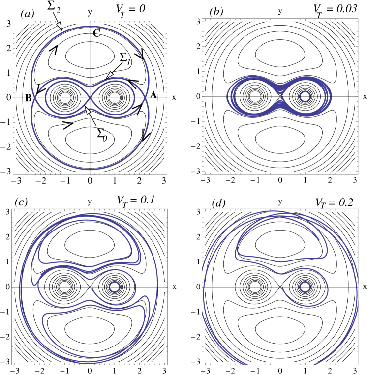
Figure 2: Streamlines in the rotating frame (a). Trajectories of two inertia-free particles for various terminal velocities (b)(c)(d). The particle injected near the vortex has a regular trajectory around it. In contrast, the particle injected near the separatrix $\Sigma_{0}$ wanders in various places of the flow domain.

where the streamfunction is given by $\psi(x,y)=-2\ln|z^{2}-1|+(x^{2}+y^{2})/2$ (and $z=x+i\,y$) for the inviscid vortex pair considered here. The former term in $\psi$ is the flow induced by the two vortices, and the latter corresponds to the opposite of the velocity of the rotating frame relative to the laboratory frame. The curl of $\vec{V}_{f}$ is equal to $-2\vec{e}_{z}$ everywhere, except at the vortex centres where it is infinite. The corresponding streamlines are plotted in Fig. 2(a) : they take the classical form of an eight shape around the location of the vortices $(\pm 1,0)$. This phase portrait has three hyperbolic saddle points located at $(0,0)$ and A = $(\sqrt{5},0)$ and B = $(-\sqrt{5},0)$. The point $(0,0)$ has two homoclinic trajectories, whereas the two other points are related by a set of heteroclinic trajectories forming two heteroclinic cycles. Because this flow is two-dimensional and steady, no chaotic fluid point trajectories are expected to emerge. However, it will be shown in the next sections that the motion of particles has complex and unexpected features in such a flow.

Three situations are examined. In section 2 we examine the case $\tau=0$ and $0<V_{T}\ll 1$, where inertia is negligible and a chaotic motion takes place under the effect of the unsteady term due to gravity in Eq. (2). Then we focus on the case $0<\tau\sim V_{T}\ll 1$ and examine the effect of weak particle inertia on chaotic sedimentation (section 3). The case $V_{T}=0$ and $\tau>0$ is treated in section 4 : it will be shown that non-sedimenting inertial particles have equilibrium positions in the rotating frame, two of which are stable. A numerical experiment, taking into account the viscous diffusion of the vortices, is shown in the last paragraph of section 4.

2 Chaotic sedimentation of inertia-free particles

The case of non-inertial sedimenting particles can be addressed by assuming $\tau\to 0$ in the particle motion equation (2), so that all inertia forces vanish to leading order. In addition, we assume that $V_{T}$ is small but non-zero. We then recover the simplest motion equation for heavy particles in fluid :

$$\frac{d\vec{X}_{p}}{dt}=\vec{V}_{f}(\vec{X}_{p})-V_{T}\vec{e}_{y0}(t)$$ (3)

which has been widely used so far (see for example Stommel [17]). The particle dynamics therefore corresponds to a steady two-dimensional flow ($\vec{V}_{f}$), plus a time-periodic perturbation due to gravity. The dynamical system (3), in the absence of perturbation ($V_{T}=0$), has a homoclinic trajectory and a heteroclinic cycle : it is therefore tempting to check whether or not a finite perturbation ($0<V_{T}\ll 1$) induces a homoclinic bifurcation, leading to chaotic aerosol motion in the vortex system. This point can be readily addressed by calculating the Melnikov function of any of these separatrices (say, $\Sigma_{i}$) :

$$M_{i}(t_{0})=-\int_{-\infty}^{+\infty}\frac{d\vec{X}_{0}}{dt}\times\vec{e}_{y0}(t+t_{0})\,dt$$

where $t_{0}$ is the starting time of the Poincaré section of the perturbed system (i.e. $T$-stroboscopy of the system with $T=2\pi/\Omega$) and $\vec{X}_{0}(t)$ is the solution of the undisturbed system corresponding to a point moving along the separatrix $\Sigma_{i}$ (see for example Guckenheimer & Holmes [8]), that is :

$$\frac{d\vec{X}_{0}}{dt}=\vec{V}_{f}(\vec{X}_{0}(t))$$ (4)

If the Melnikov function has simple zeros when $t_{0}$ varies, then the Poincaré application of the system (or one of its iterates) corresponds to a horse-shoe map, and the particle dynamics is chaotic in the vicinity of $\Sigma_{i}$ (Smale-Birkhoff theorem). For the homoclinic trajectory $\Sigma_{0}$ the coordinates $x_{0}(t)$ and $y_{0}(t)$ of $\vec{X}_{0}$ are even and odd functions of time respectively (choosing $\vec{X}_{0}(0)$ equal to the intersection between $\Sigma_{0}$ and $Ox$). We obtain, after removing the integral of odd functions :

$$M_{0}(t_{0})=\alpha_{0}\,\sin(t_{0})$$

where

$$\alpha_{0}=\int_{-\infty}^{+\infty}\Big{(}\dot{x}_{0}(t)\,\sin t+\dot{y}_{0}(t)\,\cos t\Big{)}dt$$

and $\dot{x}_{0}$ and $\dot{y}_{0}$ are the coordinates of $d\vec{X}_{0}/dt$. For the heteroclinic trajectories $\Sigma_{1}$ and $\Sigma_{2}$ the coordinates $x_{0}(t)$ and $y_{0}(t)$ of $\vec{X}_{0}$ are odd and even functions of time respectively (choosing $\vec{X}_{0}(0)$ equal to the intersection between the separatrix and $Oy$.) We obtain, once again removing the integral of odd functions :

$$M_{i}(t_{0})=\alpha_{i}\,\cos(t_{0})$$

where

$$\alpha_{i}=\int_{-\infty}^{+\infty}\Big{(}-\dot{x}_{0}(t)\,\cos t+\dot{y}_{0}(t)\,\sin t\Big{)}dt.$$

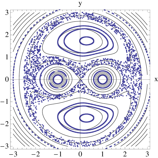
Figure 3: Poincaré section of 20 inertia-free particles, for $V_{T}=0.03$.

for $i=1$ and $i=2$. In order to obtain the coordinates of $\vec{X}_{0}(t)$ we need to solve (4), with the appropriate initial conditions specified above, on $\Sigma_{i}$. The equation of the separatrix $\Sigma_{i}$ reads $-2\ln|z^{2}-1|+r^{2}/2=\psi(\Sigma_{i}),$ where $r=|z|$. By injecting this last equation into the undisturbed system (4) we are led to a purely numerical differential system which can be solved numerically to obtain $x_{0}(t)$ and $y_{0}(t)$. From these the above integrals can be calculated and we get $\alpha_{0}\approx-1.6$, $\alpha_{1}\approx 1.7$ and $\alpha_{2}\approx-5.8$. Hence, the Melnikov functions of the three separatrices have simple zeros. We therefore conclude that, as soon as gravity is taken into account, a bifurcation occurs in the particle dynamics and chaotic trajectories exist in the vicinity of the homoclinic trajectory $\Sigma_{0}$ and of the heteroclinic cycle $\Sigma_{1}\cup\Sigma_{2}$. Numerical solutions of equation (3) confirm this result : Fig. 2 shows the trajectory of two particles injected respectively near the separatrix $\Sigma_{0}$ and near the right-hand-side vortex. When $V_{T}=0$ these particles follow the streamlines, since the flow is steady. When $V_{T}$ increases the particle injected near the separatrix has a very complex trajectory : it rotates in a chaotic manner around both vortices alternatively, as a consequence of the breaking of $\Sigma_{0}$. In contrast, the other particle, injected in a non-chaotic zone, has a regular trajectory around the same vortex. For higher $V_{T}$’s the former particle wanders in several places of the domain. The Poincaré sections of 20 particle trajectories, computed over 100 periods, are shown in figure 3, for $V_{T}=0.03$. A stochastic zone is clearly visible in the vicinity of $\Sigma_{0}$ and $\Sigma_{1}\cup\Sigma_{2}$, in agreement with the Melnikov theory presented in this paragraph.

3 Effect of inertia on chaotic sedimentation

When particle inertia, though small, is no longer negligible compared to gravity effects, that is if :

$$0<\tau\sim V_{T}\ll 1$$

i.e. the Froude number $\mbox{Fr}=d\Omega^{2}/g$ is of order unity, then the particle motion equation (2) can be solved approximately by looking for an asymptotic solution of the form (Michael [4], Maxey [13]) ${d\vec{X}_{p}}/{dt}=\vec{V}_{f}(\vec{X}_{p})+\tau\vec{V}^{1}+O(\tau^{2}),$ and keeping Fr as a fixed parameter as $\tau\to 0$. We are led to :

$$\frac{d\vec{X}_{p}}{dt}=\vec{V}_{f}(\vec{X}_{p})+\tau\Big{[}-\frac{1}{\mbox{Fr}}\,\vec{e}_{y0}(t)-\overline{\overline{\nabla}}\vec{V}_{f}.\vec{V}_{f}+\vec{X}_{p}-2\vec{e}_{z}\times\vec{V}_{f}\Big{]}+O(\tau^{2})$$ (5)

Like in the previous section we recover a non-autonomous dynamical system with two degrees of freedom (the phase space being the physical space), in the form of a perturbed hamiltonian system. The perturbation is now dissipative and contains the gravity term, the inertia term, the centrifugal and the Coriolis forces. The Melnikov function of a separatrix $\Sigma_{i}$ now reads :

$$M_{i}(t_{0})=-\frac{1}{\mbox{Fr}}\int_{-\infty}^{+\infty}\frac{d\vec{X}_{0}}{dt}\times\vec{e}_{y0}(t+t_{0})\,dt+m_{i}$$

where :

$$m_{i}=\int_{-\infty}^{+\infty}\frac{d\vec{X}_{0}}{dt}\times\Big{(}-\frac{d^{2}\vec{X}_{0}}{dt^{2}}+\vec{X}_{0}(t)-2\vec{e}_{z}\times\frac{d\vec{X}_{0}}{dt}\Big{)}$$ (6)

and $\vec{X}_{0}(t)$, running on $\Sigma_{i}$, has exactly the same expression as in the previous section (solution of equation (4)). Hence, the calculation of the $t_{0}$-dependent part of the Melnikov function is straightforward. For the separatrix $\Sigma_{0}$ the Melnikov function reads :

$$M_{0}(t_{0})=\frac{1}{\mbox{Fr}}\,\alpha_{0}\,\sin(t_{0})+m_{0}$$

where $\alpha_{0}<0$ has been calculated in the previous section (for $\Sigma_{1}$ and $\Sigma_{2}$ simply replace $\alpha_{0}$ by $\alpha_{i}$ ($i=1,2$), $m_{0}$ by $m_{i}$ ($i=1,2$) and $\sin$ by $\cos$). The parameter $m_{i}$ is a constant, and manifests the effect of particle inertia on the dynamics. The Melnikov function $M_{i}(t_{0})$ has simple zeros if

$$\mbox{Fr}<\frac{|\alpha_{i}|}{|m_{i}|}=\mbox{Fr}_{i},$$ (7)

leading to chaotic particle dynamics in the vicinity of $\Sigma_{i}$. By injecting the numerical $\vec{X}_{0}(t)$ calculated above into Eq. (6), we get, for each separatrix : $m_{0}\approx-42$, $m_{1}\approx-26$ and $m_{2}\approx 8$. Because Fr, $\alpha_{0}$ and $\alpha_{1}$ are of order unity, we conclude that inertia has a huge effect on $\Sigma_{0}$ and $\Sigma_{1}$, as it tends to prevent the occurrence of simple zeros in their Melnikov function. Instead of the chaotic trajectories observed in the inertia-free limit, a regular centrifugation will take place in the vicinity of $\Sigma_{0}$ and $\Sigma_{1}$. The effect of inertia is less significant for $\Sigma_{2}$. These calculations show that as soon as

$$\mbox{Fr}>\max_{i}\mbox{Fr}_{i}=\mbox{Fr}_{2}\approx 0.7,$$

the stochastic layer around $\Sigma_{2}$ will vanish also.

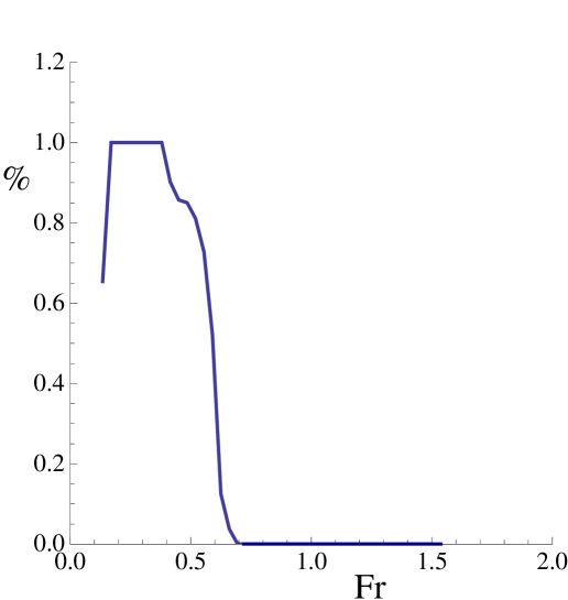
Figure 4: Plot of the percentage of particles released at $t=0$ slightly above $\Sigma_{2}$, and crossing $\Sigma_{2}$ during the simulation (the final time is $t=100$). As soon as $\mbox{Fr}>\mbox{Fr}_{2}$ the stochastic layer located in the vicinity of $\Sigma_{2}$ vanishes and no particle crosses $\Sigma_{2}$, in agreement with the Melnikov analysis.

In order to check this result we have solved numerically Eq. (5), for 1000 particles released slightly above $\Sigma_{2}$ (near point C of Fig. 2(a)), with $\tau=0.005$ and $\mbox{Fr}\in[0.1,1.5]$ (Fig. 4). If a stochastic layer exists around $\Sigma_{2}$, then some particles are likely to penetrate inside the zone bounded by $\Sigma_{2}\cup\Sigma_{1}$. These particles are those who are located in the lobes formed between every two intersection point of the unstable manifold $W^{u}(B)$ (coming out of the hyperbolic point located near point B of Fig. 2(a)) and the stable manifold $W^{s}(A)$ (converging to the hyperbolic point located near A). We observe on Fig. 4 that some particles indeed penetrate inside the zone bounded by $\Sigma_{2}\cup\Sigma_{1}$ for $\mbox{Fr}<\mbox{Fr}_{2}$. The detailed shape of the curve for $\mbox{Fr}<\mbox{Fr}_{2}$ depends on the shape and position of the initial cloud. As soon as $\mbox{Fr}>\mbox{Fr}_{2}$ however, the curve is flat and no particle penetrate into the zone bounded by $\Sigma_{1}\cup\Sigma_{2}$, in agreement with the Melnikov analysis. Indeed, when $\mbox{Fr}>\mbox{Fr}_{2}$ the Melnikov function $M_{2}(t_{0})$ is constant and non-zero, so that $W^{s}(A)$ and $W^{u}(B)$ never intersect, and particles located outside cannot penetrate into the zone bounded by $\Sigma_{2}\cup\Sigma_{1}$.

4 Trapping of non-sedimenting inertial particles

When the particle response time is of order unity and gravity effects are small ($V_{T}\ll\tau=O(1)$), particles are expected to be centrifugated away from the vortices. Here we show that this is not always the case, and that some particles, in spite of their finite inertia, can be trapped and remain in the vicinity of the vortex system. For the sake of simplicity we assume that the gravity term in the particle motion equation (2) can be neglected, so that the fluid velocity field in the rotating frame is now steady. By using this simplification we notice that (2) has equilibrium points where the centrifugal pseudo-force balances the Stokes drag :

$$\vec{0}=\vec{V}_{f}(\vec{X}_{p})+\tau\,\vec{X}_{p}.$$ (8)

If one of these points were asymptotically stable, which is the case if all the corresponding eigenvalues have strictly negative real parts, some particles could be trapped there and remain fixed in the rotating frame. This would imply permanent trapping by the vortex pair. In order to clarify this point we analyze, in the following lines, the equilibrium points and their stability.

The equilibrium equation has a trivial solution, $\vec{X}_{p}^{(1)}=(0,0)$, for all $\tau$. By re-writing equation (8) in polar coordinates $(r,\theta)$, and after a few algebra (see appendix A), we obtain four more equilibrium points if $0<\tau<2-\sqrt{3}$ or $\tau>2+\sqrt{3}$. These points are symmetric with respect to $(0,0)$ and are denoted $\pm\vec{X}_{eq}^{(2)}$ and $\pm\vec{X}_{eq}^{(3)}$. They correspond to

$$\sin 2\theta=\frac{4\tau}{\tau^{2}+1}$$

that is, $\theta_{2}=\arcsin(4\tau/(\tau^{2}+1))\,/2$ (mod $\pi$) and $\theta_{3}=\pi/2-\theta_{2}$ (mod $\pi$). The coordinate $r$ of these points is given by $r^{2}=(\sin 2\theta)/\tau+\cos 2\theta$, that is :

$$r^{2}=\frac{1}{\tau^{2}+1}(4\pm\sqrt{\tau^{4}-14\tau^{2}+1})$$ (9)

The stability of these points can be addressed by re-writing the motion equation (2), with $V_{T}=0$, as a standard dynamical system with four degrees of freedom, with state variable $\vec{Y}=(x,y,\dot{x},\dot{y})$, where $(x,y)$ denote the coordinates of the particle. Then (2) is an autonomous system of the form $d\vec{Y}/dt=\vec{F}(\vec{Y})$. One can check, by studying the roots of the characteristic polynomial of the Jacobian matrix $\nabla\mathbf{F}=(\partial F_{i}/\partial Y_{j})$ at the equilibrium points, that $\pm\vec{X}_{eq}^{(2)}$ is always unstable (see appendix B). Let us now consider the equilibrium point $\vec{X}_{eq}^{(3)}$. The determinant of $\nabla\mathbf{F}$ at $\vec{X}_{eq}^{(3)}$ is :

$$\Delta(\vec{X}_{eq}^{(3)})=-\frac{1}{4\tau^{2}}\left(\tau^{4}-14\tau^{2}+1-4(\tau^{4}-14\tau^{2}+1)^{1/2}\right)$$ (10)

It is negative only if $\tau^{4}-14\tau^{2}+1>16$, that is $\tau>\sqrt{15}$. Hence, by applying the same arguments as before, we conclude that for $\tau>\sqrt{15}$ this equilibrium point is also unstable. However, for smaller $\tau$, and in particular for all $\tau$ in the range $0<\tau<2-\sqrt{3}$, we have $\Delta(\vec{X}_{eq}^{(3)})>0$ : the equilibrium point $\vec{X}_{eq}^{(3)}$ is not necessarily unstable. To prove that this point is indeed stable we need to solve for the characteristic polynomial of $\nabla\mathbf{F}$ at $\vec{X}_{eq}^{(3)}$, which reads :

$$P(\lambda)=\lambda^{4}+\frac{2\lambda^{3}}{\tau}+(2+\frac{1}{\tau^{2}})\lambda^{2}+\frac{2\lambda}{\tau}+\Delta$$

where $\Delta(\tau)$ simply denotes $\Delta(\vec{X}_{eq}^{(3)})$. By setting $z=\lambda+1/(2\tau)$ we are led to a simpler polynomial :

$$P(\lambda)=\tilde{P}(z^{2})=\frac{16\tau^{4}z^{4}+8\tau^{2}(4\tau^{2}-1)z^{2}+8\tau^{2}(2\tau^{2}\Delta(\tau)-1)+1}{16\tau^{4}}$$

which can be readily solved. We obtain :

$$z^{2}_{\pm}=\frac{1-4\tau^{2}\pm 4\tau^{2}\sqrt{1-\Delta(\tau)}}{4\tau^{2}}$$

Because we consider the case $\Delta>0$, two cases emerge : $0<\Delta<1$ and $\Delta>1$. In the former case ($0<\Delta<1$) then $z^{2}_{\pm}$ are real. Clearly, we have $z^{2}_{-}<1/(4\tau^{2})$. If $z^{2}_{-}<0$ then $z_{-}$ is pure imaginary and the two corresponding $\lambda$’s have a negative real part equal to $-1/2\tau$. If $z^{2}_{-}>0$ then $z_{-}<1/(2\tau)$, so $\lambda<0$. The second pair of roots are given by :

$$z^{2}_{+}=\frac{1+4\tau^{2}(\sqrt{1-\Delta(\tau)}-1)}{4\tau^{2}}<1/(4\tau^{2})$$

since $\sqrt{1-\Delta(\tau)}-1<0$. Here also we conclude that the corresponding eigenvalues of $\nabla\mathbf{F}$ are real negative (or are complex with negative real parts if $z^{2}_{+}<0$).

We now turn to the case $\Delta>1$. By setting $a=Re(z)$ we are led to $a^{2}=(Re(z^{2})+|z^{2}|)/2$ and :

$$4\tau^{2}a^{2}=(1-4\tau^{2}+(1-8\tau^{2}+16\tau^{4}\Delta(\tau))^{1/2})/2$$ (11)

One can prove that the function of $\tau$ appearing at the rhs of this equation is always smaller than 1 (see appendix C). Therefore, $a<1/(2\tau)$, and the corresponding eigenvalues of $\nabla\mathbf{F}$ satisfy $Re(\lambda)=a-1/(2\tau)<0$.

We therefore conclude that, for all $\tau$ in the range $0<\tau<2-\sqrt{3}$, there exists a pair of asymptotically stable points located at $\pm\vec{X}^{(3)}_{eq}$.

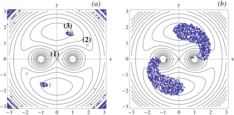
Figure 5: (a) : plot of a particle cloud after 20 convective times. At $t=0$ the cloud covers the square $[-3,3]^{2}$, and is composed of inertial particles with $\tau=0.2$ and $V_{T}=0$. The equilibrium points $\vec{X}^{(i)}_{eq}$ are indicated by the white dots (i). Graph (b) shows the initial position of trapped particles.

In order to check these results, and to illustrate the effect of the attracting points $\pm\vec{X}_{eq}^{(3)}$ on the particle dynamics, we have computed the trajectories of 10000 particles injected at $t=0$ in the square $[-3,3]^{2}$, for $\tau=0.2$. Results are shown in figure 5 where the particle cloud is plotted. Graph (a) shows that trapping indeed occurs, and that some particles converge to the points $\pm\vec{X}^{(3)}_{eq}$ predicted by the theory. Also, graph (b) shows the initial position of all particles such that $|\vec{X}_{p}\pm\vec{X}^{(3)}_{eq}|<0.2$ at $t=20$ : it gives an approximate view of a 2D cut, in the $(x,y$) plane, of the basin of attraction of the equilibrium points $\vec{X}^{(3)}_{eq}$ and $-\vec{X}^{(3)}_{eq}$.

In addition, we have conducted a series of runs, where 2000 particles were injected at $t=0$ all over the square $[-3,3]^{2}$, for various response times $\tau$. We then have computed the percentage of particles lying inside the disk of radius 2 and centre (0,0) at long times (here $t=50$). Most of these particles are those which have been "trapped" by the two attracting points, if any. Clearly, in the absence of attracting points $p(\tau)\approx 0$, whereas $p(\tau)$ is finite if attracting points are present. So, if $\tau$ is not too small this percentage is a good indicator of the occurrence of trapping. Figure 6 shows that, as soon as $\tau>2-\sqrt{3}$, the percentage is identically 0, in agreement with the stability analysis : the determinant is negative there, so that the point $\pm\vec{X}_{eq}^{(3)}$ is unstable.

Comparison with a numerical experiment. These results are valid for inviscid fluids. When viscosity is finite the flow is significantly different since vortices coalesce and finally form a single vortex. Particles will therefore be centrifugated away once coalescence occurs. However, if the diffusive time scale over $d$ is larger than the turnover time $\Omega^{-1}$, one can expect particles to be trapped temporarilly in the vicinity of $\pm\vec{X}_{eq}^{(3)}$ (the stable points of the inviscid flow investigated above) during the interaction of the vortices, even though the equilibrium points do not exist strictly speaking since the relative flow is no longer steady. We have therefore performed a series of runs with a two-dimensional (spectral) Navier-Stokes solver including a lagrangian particle tracking algorithm, within a periodic box $[-\pi d,\pi d]^{2}$. The initial condition corresponds to a pair of Lamb-Oseen vortices $\vec{V}_{f}(x,y)=(-\omega(r)y,\omega(r)(x-x_{v}))$ with

$$\omega=\Gamma[1-\exp(-3r^{2}/\delta^{2})]/(2\pi r^{2})$$

where $r^{2}=(x-x_{v})^{2}+y^{2}$ and $x_{v}=\pm d$ is the initial $x$-coordinate of the vortices. The circulation of a single vortex of this kind, placed in an infinite domain, is independent of the core thickness $\delta$ and is equal to $\Gamma$. The fluid and particle motion equations are set non-dimensional by using $\Omega^{-1}=4\pi d^{2}/\Gamma$ for times and $d$ for scales, like for the inviscid calculations presented above. The initial core-size $\delta$ of the vortices is taken to be one tenth of the flow domain. The Reynolds number $Re=\Omega d^{2}/\nu$ is equal to 800. The number of Fourier modes is 256 in each direction, and a second-order Adams-Bashforth algorithm is used for time stepping. Particles are passive (they do not modify the flow), and do not interact. They are injected at random at $t=0$ and cover the whole vortex pair. Their initial velocity is equal to that of the fluid, and their trajectories are calculated by solving equation (2) (without the inertia forces since the numerical solver used here considers the dynamical equations in the laboratory reference frame).

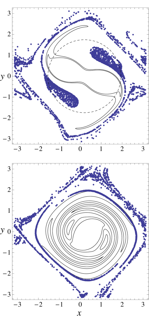
Figure 7: Evolution of a particle cloud (in the laboratory frame) advected by a vortex pair at large but finite Reynolds number, for $\tau=0.1$ and $V_{T}=0$. Lines are vorticity contours. Upper figure : $t=10$, lower figure : $t=15$.

Figure 7 shows the evolution of the vortices and of the particle cloud, when $\tau=0.1$ (this value has been chosen because it corresponds to the peak of figure 6). We observe that particle trapping indeed occurs, and persists until $t\approx 12$ (that is about two turns). Because this calculation is done in a periodic domain, the influence of the neighbouring vortex pair located in boxes $[-\pi+2n\pi,\pi+2n\pi]^{2},\,n\in\mathbf{Z}$ is significant here. However, these vortices do not prevent the appearance of the attracting points predicted by the inviscid theory in infinite domain (section 4). When coalescence begins, the set of trapped particles is elongated into a thin filament (Fig. 7) which will then be centrifugated away. The dashed line in figure 7 is the trajectory of the relative equilibrium points $\pm\vec{X}_{eq}^{(3)}$ of the inviscid theory (equation (9)). This line is close to the position of the accumulation points, in spite of the effect of viscosity and of the neighbouring vortices.

5 Conclusion and open questions

We have investigated the motion of tiny heavy particles with or without inertia and gravity in a co-rotating vortex pair. For sedimenting inertia-free particles ($\tau=0$ and $0<V_{T}\ll 1$) we have shown that, under the combined effect of gravity and of the rotation of the vortices, a chaotic particle dynamics can take place. By writing the particle motion equation in the rotating reference frame attached to the vortices, we observed that the particle dynamics take the form of a hamiltonian system submitted to a periodic forcing due to gravity. A "stretch-sediment and fold" mechanism is responsible for this chaotic particle dynamics, like the one described in Ref. [1], as gravity plays a central role in the folding of volume elements of the dispersed phase.

Chaotic motion is very sensitive to particle inertia when $0<\tau\sim V_{T}\ll 1$. Indeed, by using nearly hamiltonian dynamical system theory for the particle motion equation written in the rotating reference frame, we have shown that small inertia terms of the particle motion equation strongly modify the Melnikov function of the homoclinic trajectory of the unperturbed system. In particular, the stochastic layer in the vicinity of the separatrices $\Sigma_{i}$ ($i$=0,1,2) vanishes as soon as the Froude number is larger than some critical values $\mbox{Fr}_{i}$ given by equation (7). A regular centrifugation therefore takes place as soon as the Froude number is above $\max\mbox{Fr}_{i}\approx 0.7$. Numerical results confirm this value (figure 4).

Particles with a finite inertia, and in the absence of gravity ($\tau=O(1)$ and $V_{T}=0$), can have various equilibrium positions in the rotating reference frame, according to whether their Stokes number is smaller or larger than some critical values of order unity. We have rigorously shown that two of these points are stable attracting points, so that permanent trapping occurs for inertial particles injected in an isolated co-rotating vortex pair. Numerical computations confirm this result, and show that the basin of attraction of the attracting points covers a non-negligible part of the flow domain. Our analytical calculations also show that trapping should stop if $\tau$ exits the range $0<\tau<2-\sqrt{3}$. This point has been confirmed by computing the percentage of trapped particles (which can be thought of as a measure of the basin of attraction), for various reponse times $\tau$ : this percentage drops to 0 as soon as $\tau>2-\sqrt{3}$. Note that the points $\pm\vec{X}_{eq}^{(2)}$ and $\pm\vec{X}_{eq}^{(3)}$ also exist for $\tau>2+\sqrt{3}$. However, the former has been shown to be unstable for all $\tau$, and the latter is also unstable as soon as $\tau>\sqrt{15}$. Numerical experiments taking into account the effect of viscosity have been conducted. We observe that, when the Reynolds number $\Omega d^{2}/\nu$ is large, the effects of viscosity are sufficiently slow to enable particle trapping in the vicinity of two points, the position of which is in qualitative agreement with the results of the inviscid theory. Once vortex coalescence is complete, particles are centrifugated away.

Note that this effect could be of interest also in the context of particle motion in protosellar gaseous disks. Indeed, large scale anticyclonic vortices might play a key role in dust trapping, with the help of the Coriolis force due to the disk rotation, and these vortices are known to interact and coalesce. The dynamics of dust during vortex pairing in protostellar disks could therefore be a topic of interest.

When $\tau=O(1)$ and $V_{T}$ is non-zero the flow equation is unsteady in the rotating frame, and the attracting equilibrium points described above no longer exist. The analytical treatment of particle dynamics in this case is much more complex, but numerical simulations, not shown here, suggest that trapping could exist anyway. Further analyses should clarify this point.

The generalization of these results to vortex pairs with different strengths is the next step of this work. Preliminary numerical simulations show that particle trapping still exists in the asymetric case, but the analytical treatment is heavier and is currently under study. Also, when vortices are located in the vicinity of a wall and move parallel to it, particle trapping is expected to persist. Indeed, Vilela & Motter [19] have observed attracting points in their simulation of particle transport in a leapfrogging vortex system (which also corresponds to a 2D inviscid vortex pair in the vicinity of a wall). We therefore conclude that the attracting points persist in the presence of the wall, even though these points have a more complicated trajectory. A detailed theoretical analysis would enable to determine the range of parameters leading to such a trapping.

Appendix A Equilibrium positions of inertial particles

The equilibrium equation (8) reads

$$\frac{-4y(r^{2}+1)}{r^{4}+1+2(y^{2}-x^{2})}+y+\tau x = 0,$$ (12)

$$\frac{4x(r^{2}-1)}{r^{4}+1+2(y^{2}-x^{2})}-x+\tau y = 0$$ (13)

where $r^{2}=x^{2}+y^{2}$. By using polar coordinates, and combining these two equations, we are led to :

$$r^{2}=(\sin 2\theta)/\tau+\cos 2\theta,$$ (14)

together with the admissibility condition required to avoid a null denominator :

$$r^{4}+1-2r^{2}\cos 2\theta\not=0$$ (15)

By injecting this $r$ into (12)-(13) we get :

$$\sin 2\theta\,(\tau\sin\theta-\cos\theta)\left[(1+\tau^{2})\sin 2\theta-4\tau\right]=0$$

and

$$\sin 2\theta\,(\sin\theta+\tau\cos\theta)\left[(1+\tau^{2})\sin 2\theta-4\tau\right]=0$$

Because $\tau\sin\theta-\cos\theta$ and $\sin\theta+\tau\cos\theta$ cannot be both zero, two families of solutions emerge. The first one is $\sin 2\theta=0$ and $r=1$ : it does not satisfy the admissibility condition (15), and must be rejected. The second one exists if $1+\tau^{2}>4\tau$, that is $0<\tau<2-\sqrt{3}$ or $\tau>2+\sqrt{3}$, and corresponds to :

$$\sin 2\theta=\frac{4\tau}{1+\tau^{2}},$$

that is $\theta_{0}=\arcsin(\frac{4\tau}{1+\tau^{2}})/2$, and $\theta=\pi+\theta_{0}$, and $\theta=\pi/2-\theta_{0}$, and $\theta=3\pi/2-\theta_{0}$ (mod $\pi$). These angles corresponds to 4 equilibrium positions in the physical plane, denoted $\pm\vec{X}_{eq}^{(2)}$ and $\pm\vec{X}_{eq}^{(3)}$. The $r$ coordinates of these points are obtained by using (14).

Appendix B Instability of equilibrium point (2).

The determinant $\Delta(\vec{X}_{eq}^{(2)})$ of $\nabla\mathbf{F}$ at $\vec{X}_{eq}^{(2)}$ is :

$$\Delta(\vec{X}_{eq}^{(2)})=-\frac{1}{4\tau^{2}}\left(\tau^{4}-14\tau^{2}+1+4(\tau^{4}-14\tau^{2}+1)^{1/2}\right)$$

and one can check, since $2\pm\sqrt{3}$ are also roots of $\tau^{4}-14\tau^{2}+1$, that $\tau^{4}-14\tau^{2}+1$ is strictly positive for all $\tau$ such that $0<\tau<2-\sqrt{3}$ or $\tau>2+\sqrt{3}$. We then conclude that $\Delta(\vec{X}_{eq}^{(2)})$ is always negative in this range of $\tau$. This implies that the equilibrium point $\vec{X}_{eq}^{(2)}$ is unstable.

Indeed, let $\lambda_{i}$, ($i=1,...,4$) be the roots of the characteristic polynomial of $\nabla\mathbf{F}$ at $\vec{X}_{eq}^{(2)}$. Because the coefficients of the polynomial are real these roots are either real or complex conjugate. Also $\lambda_{1}\lambda_{2}\lambda_{3}\lambda_{4}=\Delta(\vec{X}_{eq}^{(2)})<0$. Clearly, this implies that the four roots cannot be complex conjugates (i.e. $\lambda_{2}=\bar{\lambda}_{1}$ and $\lambda_{4}=\bar{\lambda}_{3}$) since we would have $\Delta(\vec{X}_{eq}^{(2)})=|\lambda_{1}|^{2}\,|\lambda_{3}|^{2}>0$ there. If two of these roots (say $\lambda_{1}$ and $\lambda_{2}$) are complex conjugates and the other two are real, then we must have $|\lambda_{1}|^{2}\lambda_{3}\lambda_{4}<0$, so $\lambda_{3}\lambda_{4}<0$ : hence there exists a strictly positive eigenvalue : the equilibrium point is unstable. Finally, if all the roots are real, then, their product being strictly negative, one of them at least is positive : $\vec{X}_{eq}^{(2)}$ is unstable.

Appendix C Upper bound for $Re(z)^{2}$

To prove that $a^{2}<1/(4\tau^{2})$ we need to show that (Eq. (11)) :

$$1-4\tau^{2}+(1-8\tau^{2}+16\tau^{4}\Delta(\tau))^{1/2}<2$$

for all $\tau$ in the range $0<\tau<2-\sqrt{3}$. This is equivalent to :

$$(1-8\tau^{2}+16\tau^{4}\Delta(\tau))^{1/2}<1+4\tau^{2}$$

Taking the square of these positive numbers, and after simplifications, we are led to :

$$\tau^{2}\Delta<1+\tau^{2}$$

From (10) we get $\Delta=(-q+4\sqrt{q})/(4\tau^{2})$, with $q=\tau^{4}-14\tau^{2}+1$. The last inequality is therefore equivalent to :

$$\sqrt{q}<\frac{q}{4}+1+\tau^{2}$$

Once again, taking the square of these positive numbers, we are led to an equivalent expression :

$$q-(\frac{q}{4}+1+\tau^{2})^{2}<0$$

Because $q=\tau^{4}-14\tau^{2}+1$ we have:

$$q-(\frac{q}{4}+1+\tau^{2})^{2}=[-9-124\tau^{2}-\tau^{4}(94-20\tau^{2})-\tau^{8}]/16$$

and this last quantity, being a sum of negative numbers (since $0<\tau<2-\sqrt{3}$), is negative. We therefore conclude that $a^{2}<1/(4\tau^{2})$.

Figure 1: Sketch of the two vortices (black dots), together with the rotating reference frame with axes $(O,x,y)$ and the laboratory frame with axes $(O,x_{0},y_{0})$. The lower graph is the homoclinic trajectory of the fluid points dynamics in the rotating frame.

Figure 6: Plot of the percentage of "trapped" particles at $t=50$, versus $\tau$, when $V_{T}=0$. As soon as $\tau>2-\sqrt{3}\approx 0.27$ no trapping is observed ($p(\tau)=0$), in agreement with the stability analysis.

References

- [1] J.R. ANGILELLA. Chaotic particle sedimentation in a rotating flow with time-periodic strength. Phys. Rev. E, 78(16):066310, 2008.
- [2] R. CHEIN and J.N. CHUNG. Effects of vortex pairing on particle dispersion in turbulent shear flows. Journal of Multiphase Flow, 13(6):785–802, 1987.
- [3] J. DAVILA and J. HUNT. Settling of small particles near vortices and in turbulence. J. Fluid Mech., 440:117–145, 2001.
- [4] MICHAEL D.H. The steady motion of a sphere in a dusty gas. J. Fluid Mech., 31:175–192, 1968.
- [5] O.A. DRUZHININ. The dynamics of a concentration interface in a dilute suspension of solid heavy particles. Phys. Fluids, 9(2):315–324, 1997.
- [6] A. FERRANTE and S. ELGHOBASHI. On the physical mechanisms of two-way coupling in particle-laden isotropic turbulence. Phys. Fluids, 15(2):315–329, 2003.
- [7] J.C.H. FUNG. Gravitational settling of small spherical particles in unsteady cellular flow fields. J. Aerosol Sci., 5:753–787, 1997.
- [8] J. GUCKENHEIMER and P. HOLMES. Non-linear oscillations, dynamical systems and bifurcation of vector fields. 1983. Springer.
- [9] G. HALLER and T. SAPSIS. Where do inertial particles go in fluid flows? Physica D, 237(5):573–583, 2008.
- [10] K. T. KIGER and LASHERAS J. C. The effect of vortex pairing on particle dispersion and kinetic energy transfer in a two-phase turbulent shear layer. J. Fluid Mech., 302:149–178, 1995.
- [11] J.B. MACLAUGHLIN. Particle size effects on lagrangian turbulence. Phys. Fluids, 31(9):2544–2553, 1988.
- [12] E. MARCU, B. MEIBURG and P.K. NEWTON. Dynamics of heavy particles in a Burgers vortex. Phys. Fluids, 7(2):400–410, February 1995.
- [13] M. R. MAXEY. The gravitational settling of aerosol particles in homogeneous turbulence and random flow fields. J. Fluid Mech., 174:441–465, 1987.
- [14] M. R. MAXEY and S. CORRSIN. Gravitational settling of aerosol particles in randomly oriented cellular flow fields. J. Atmos. Sci., 43(11):1112–1134, 1986.
- [15] N. RAJU and E. MEIBURG. The accumulation and dispersion of heavy particles in forced two-dimensional mixing layers. part 2: the effect of gravity. Phys. Fluids, 7(6):1241–1264, 1995.
- [16] J. RUBIN, C.K.R.T. JONES, and M. MAXEY. Settling and asymptotic motion of aerosol particles in a cellular flow field. J. Nonlinear Sci., 5:337–358, 1995.
- [17] H. STOMMEL. Trajectories of small bodies sinking slowly through convection cells. J. Marine Res., 8:24–29, 1949.
- [18] Y. TSEGA, E. MICHAELIDES, and E.V. ESCHENAZI. Particle dynamics and mixing in the frequency driven kelvin cat eyes flow. Chaos, 11(2):351–358, 2001.
- [19] R.D. VILELA and A. E. MOTTER. Can aerosols be trapped in open flows ? Phys. Rev. Let., 99(264101), 2007.
- [20] L.P. WANG, M.R. MAXEY, T.D. BURTON, and STOCK D.E. Chaotic dynamics of particle dispersion in fluids. Phys. Fluids A, 4(8):1789–1804, 1992.