Efficient cosmological parameter sampling using sparse grids

Abstract

We present a novel method to significantly speed up cosmological parameter sampling. The method relies on constructing an interpolation of the CMB-log-likelihood based on sparse grids, which is used as a shortcut for the likelihood-evaluation. We obtain excellent results over a large region in parameter space, comprising about 25 log-likelihoods around the peak, and we reproduce the one-dimensional projections of the likelihood almost perfectly. In speed and accuracy, our technique is competitive to existing approaches to accelerate parameter estimation based on polynomial interpolation or neural networks, while having some advantages over them. In our method, there is no danger of creating unphysical wiggles as it can be the case for polynomial fits of a high degree. Furthermore, we do not require a long training time as for neural networks, but the construction of the interpolation is determined by the time it takes to evaluate the likelihood at the sampling points, which can be parallelised to an arbitrary degree. Our approach is completely general, and it can adaptively exploit the properties of the underlying function. We can thus apply it to any problem where an accurate interpolation of a function is needed.

1 Introduction

The main two bottlenecks in cosmological parameter estimation using the power spectrum of the cosmic microwave background (CMB) are the calculation of the theoretical $C_{l}$-spectrum using Boltzmann codes such as CMBFAST (Seljak & Zaldarriaga, 1996), CAMB (Lewis et al., 2000), or CMBEASY (Doran, 2005) and the evaluation of the likelihood using the official WMAP likelihood code. There exist several methods to speed up the calculation of the power spectrum (Jimenez et al., 2004; Kaplinghat et al., 2002; Habib et al., 2007) or the WMAP likelihood function $\mathcal{L}$ (Sandvik et al., 2004; Fendt & Wandelt, 2007; Auld et al., 2008). These methods are based on different techniques, such as analytic approximations, polynomial fits, and neural networks, which are all trained using a set of training points, for which the real power spectra and likelihood values have to be calculated. Once the codes are trained for a particular cosmological model, they can be used to evaluate the power spectrum or the likelihood function in every subsequent parameter estimation run, which significantly speeds up the Markov Chain Monte Carlo (MCMC) simulations used for parameter estimation. Due to the ever-growing amount of available data, a fast evaluation of the likelihood is becoming of increasing importance, especially when combining CMB data with data-sets whose likelihood is less expensive to evaluate. The Planck Surveyor mission (Tauber, 2000) will be the upcoming challenge in this respect.

In this work, we approximate the WMAP log-likelihood function $\ln\mathcal{L}$ in the spirit of CMBfit (Sandvik et al., 2004) and Pico (Fendt & Wandelt, 2007), which work with polynomial fits, and CosmoNet (Auld et al., 2008), an approach based on neural networks. In contrast to the fitting functions constructed therein, we introduce the technique of sparse grids in this context to construct an interpolation of $\ln\mathcal{L}$, returning the exact function values at a set of sampling points.

Most straightforward interpolation techniques are based on sets of sampling points in each dimension, typically based on (uniform) grid structures—consider, e. g., piecewise $d$-linear or piecewise $d$-polynomial interpolation schemes. Unfortunately, grid-based methods are only feasible in low-dimensional settings, as they suffer from the so-called curse of dimensionality: Spending $\tilde{N}$ function evaluations or grid points in one dimension leads to $\tilde{N}^{d}$ grid points in $d$ dimensions. The exponential dependency on the dimensionality imposes severe restrictions on the number of dimensions that can be handled. Sparse grids, as introduced by Zenger (1991), allow to overcome the curse of dimensionality to some extent, at least for sufficiently smooth functions as it is the case in our setting. Sparse grid interpolation is based on an a priori selection of grid points, requiring significantly fewer grid points than conventional interpolation on a full grid, while preserving the asymptotic error decay of a full-grid interpolation with increasing grid resolution up to a logarithmic factor. This permits us to compute higher-dimensional interpolations and approximations than before. A very good overview about sparse grids, discussing general properties, can be found in Bungartz & Griebel (2004).

The sparse grid technique is a completely general approach, not tailored to a single application, and can therefore be used to interpolate any function which is sufficiently smooth. Additionally, as it allows for arbitrary adaptive refinement schemes, the general, fast convergence rates can be improved even further, by adapting to the special characteristics of the underlying target function.

We obtain excellent results, which are competitive to fitting procedures using polynomials (Fendt & Wandelt, 2007; Sandvik et al., 2004) or neural networks (Auld et al., 2008) in speed and accuracy. Furthermore, we believe that the interpolation based on sparse grids has several advantages over these approaches. First of all, we can use the results of sparse grid approximation quality (Bungartz & Griebel, 2004), guaranteeing the convergence of the interpolation towards the original function with increasing number of grid points.

Second, once we have chosen the volume in which we want to interpolate the function in question, the sparse grid structure itself determines a priori the location of potential sampling points (which can additionally be refined in an adaptive manner a posteriori). This makes it unnecessary to assemble a set of training points beforehand (e.g. by running MCMCs as it is done by Fendt & Wandelt (2007)). The generation of the sampling points and the construction of the interpolant can be strongly parallelised, which makes the sparse grid approach an ideal candidate for computational grid projects such as the AstroGrid. The time needed to construct the interpolant is determined almost only by the time it takes to evaluate the likelihood at the sampling points. We do not need additional training time as in the case of Auld et al. (2008).

Furthermore, polynomial fits to a set of training points run the risk of creating unphysical wiggles if the polynomial degree of the fitting function is chosen too high with respect to the amount of training points available. Using the sparse grids approach, piecewise polynomials of low degree are sufficient, as we are not fitting certain evaluation points, but rather interpolating a function. Increasing the accuracy is therefore equivalent to evaluating at more sampling points.

Sparse grids are based on a hierarchical formulation of the underlying basis functions, which can be used to obtain a generic estimate of the current approximation error while evaluating more and more sampling points. This can be directly used as a criterion for adaptive refinement as well as to stop further refinement.

Another advantage is that the projection of sparse grid interpolations can be done in a very fast and simple way. This would make sparse grids in principle a good candidate for sampling posteriors and projecting them directly, without having to use a Markov Chain approach in order to marginalise the posterior. Given that MCMCs need to determine the points sequentially and can therefore not be parallelised (apart from running several chains at the same time), it would be highly desirable to find alternatives that can be run in parallel.

We have attempted to use sparse grids in order to substitute the MCMCs in cosmological parameter estimations. In order to directly project the posterior distribution we would need to sample the posterior rather than its logarithm. Since, in general, the logarithm of a probability density function is considerably more well-behaved than the function itself, Sandvik et al. (2004), Fendt & Wandelt (2007), and Auld et al. (2008) all operate in log-space to speed up the generation of MCMCs instead. As the convergent phase of the interpolation with sparse grids sets in rather late when interpolating Gaussian functions (and thus the WMAP likelihood, which is close to a $d$-dimensional Gaussian), we restricted ourselves to the log-likelihood and thus to accelerating MCMCs, too.

The article is organised as follows. First, we describe the basics of sparse grids in Sec. 2, introducing a modification of the standard sparse grid approach, thus adapting the latter to our problem. In Sec. 3, we then present the interpolation of the WMAP likelihood for two different sets of parameters in both six and seven dimensions. We show that the results obtained for regular (non-adaptive) sparse grids are already competitive to other approaches and demonstrate how adaptive refinement can further improve the results. Sec. 4 finally concludes our work.

2 Basics of sparse grids

Standard grid-based approaches of interpolating a function $f$ exhibit the curse of dimensionality, a term going back to Bellman (1961): Any straightforward discretisation scheme which employs $\tilde{N}$ grid points (or, equivalently, degrees of freedom) in one dimension leads to $\tilde{N}^{d}$ grid points in $d$ dimensions. For reasonable $\tilde{N}$, the exponential dependency on the number of dimensions typically does not allow to handle more than four-dimensional problems.

Sparse grids are able to overcome this hurdle to some extent, requiring significantly fewer grid points than a full grid, while preserving the asymptotic error decay of full grid interpolation with increasing grid resolution up to a logarithmic factor. Sparse grids have originally been developed for the solution of partial differential equations (Zenger, 1991) and have meanwhile been applied to various problems, see Bungartz & Griebel (2004) and the references cited therein. Recent work on sparse grids includes stochastic and non-stochastic partial differential equations in various settings (von Petersdorff & Schwab, 2006; Ganapathysubramanian & Zabaras, 2007; Widmer et al., 2008), as well as applications in economics (Reisinger & Wittum, 2007; Holtz, 2008), regression (Garcke & Hegland, 2009; Garcke, 2006), classification (Bungartz et al., 2008; Garcke et al., 2001), fuzzy modelling (Klimke et al., 2006), and more. Note that (non-adaptive) sparse grids are closely related to the technique of hyperbolic crosses (Temlyakov, 1993).

In this section, we provide a brief overview of sparse grids for interpolation. For a detailed derivation of the characteristics of sparse grids, we refer to Bungartz & Griebel (2004). We start by formulating the interpolation on a conventional full grid using hierarchical basis functions, from which we then derive the interpolation on a sparse grid by omitting the basis functions contributing least to the interpolation.

2.1 General idea of interpolation on a full grid

We consider the piecewise $d$-linear interpolation of a function $f:\nolinebreak\Omega\rightarrow\mathbb{R}$ which is given only algorithmically, i.e., we have no closed form of $f$ but we can only evaluate $f$ at arbitrary points using a numerical code. As we want to discretise our domain of interest $\Omega$, we restrict $\Omega$ to a compact sub-volume of $\mathbb{R}^{d}$; here, $\Omega\equiv[0,1]^{d}$, the $d$-dimensional unit-hypercube. (For the standard approach of sparse grids techniques, we only consider functions that are zero on the boundary of the volume on which they are defined. This assumption will be dropped when we come to the interpolation of the log-likelihood of WMAP.)

To construct an interpolant $u$ of $f$, we discretise $\Omega$ via a regular grid, obtaining equidistant grid points $\textrm{{\hbox{\boldmath$x$\unboldmath}}}_{i}$, with mesh width $h_{n}=2^{-n}$ for some discretisation or refinement level $n$, at which we evaluate and interpolate $f$. If we define a suitable set of piecewise $d$-linear basis functions $\varphi_{i}(\textrm{{\hbox{\boldmath$x$\unboldmath}}})$, we can obtain $u(\textrm{{\hbox{\boldmath$x$\unboldmath}}})$ from the space of continuous, piecewise $d$-linear functions $V_{n}$ by combining them adequately as a weighted sum of basis functions, i.e.

$$f(\textrm{{\hbox{\boldmath$x$\unboldmath}}})\approx u(\textrm{{\hbox{\boldmath$x$\unboldmath}}})\equiv\sum_{i}\alpha_{i}\varphi_{i}(\textrm{{\hbox{\boldmath$x$\unboldmath}}})$$

with coefficients $\alpha_{i}$. Figure 1 sketches the idea for a one-dimensional example, using the standard nodal basis.

Figure 1: One-dimensional piecewise linear interpolation $u(x)$, dashed, of a function $f(x)$, solid, (left) by a linear combination of hat basis functions (right).

The curse of dimensionality, encountered when using a full grid, can be circumvented by a suitable choice of basis functions: We need a basis where the relevant information is represented by as few basis functions as possible. Most basis functions can then be omitted as they contribute only little to the interpolation of $f$, reducing a full grid to a sparse grid and allowing us to handle higher-dimensional functions than before. A suitable basis can be found by a hierarchical construction as introduced in the following section.

2.2 Hierarchical basis functions in one dimension

Sparse grids depend on a hierarchical decomposition of the underlying approximation spaces. Therefore, and first considering only the one-dimensional case which we will later extend to $d$ dimensions, we use the standard hat function,

$$\varphi(x)=\max(1-|x|,0)\,,$$ (1)

from which we derive one-dimensional hat basis functions by dilatation and translation,

$$\varphi_{l,i}(x)\equiv\varphi(2^{l}x-i)\,,$$ (2)

which depend on a level $l$ and an index $i$, $0<i<2^{l}$. The basis functions have local support and are centred at grid points $x_{l,i}=2^{-l}i$, at which we will interpolate $f$. Introducing the hierarchical index sets

$$I_{l}\equiv\left\{\,i\in\mathbb{N}:1\leq i\leq 2^{l}-1,i\text{~{}odd}\,\right\}\,,$$ (3)

we obtain a set of hierarchical subspaces $W_{l}$,

$$W_{l}\equiv\textrm{span}\left\{\varphi_{l,i}(x):i\in I_{l}\right\}.$$ (4)

We can then formulate the space of piecewise linear functions $V_{n}$ on a full grid with mesh width $h_{n}$ for a given level $n$ as a direct sum of $W_{l}$,

$$V_{n}=\bigoplus_{l\leq n}W_{l}\,,$$ (5)

see Figure 2. Note that all basis functions of the same subspace $W_{l}$ have the same size, shape, and compact support, that their supports are non-overlapping, and that together they cover the whole domain.

The interpolation $u(x)\in V_{n}$ can then be written as a finite sum,

$$u(x)=\sum_{l\leq n,i\in I_{l}}\alpha_{l,i}\varphi_{l,i}(x)\,,$$ (6)

where the so-called (hierarchical) surpluses $\alpha_{l,i}$ are uniquely indexed by the same level and index as the corresponding basis functions.

Figure 2: One-dimensional basis functions $\varphi_{l,i}$ and corresponding grid points $x_{l,i}$ up to level $n=3$ in the hierarchical basis (left) and the common nodal point basis (right).

2.3 Higher-dimensional interpolation on a full grid

The basis functions are extended to the $d$-dimensional case via a tensor product approach,

$$\varphi_{\textrm{{\hbox{\boldmath$l$\unboldmath}}},\textrm{{\hbox{\boldmath$i$\unboldmath}}}}(\textrm{{\hbox{\boldmath$x$\unboldmath}}})\equiv\prod_{j=1}^{d}\varphi_{l_{j},i_{j}}(x_{j})\,,$$ (7)

with the $d$-dimensional multi-indices $l$ and $i$ indicating level and index for each dimension. The other one-dimensional notations can be transferred to the arbitrary-dimensional case as well, consider, e.g. , the index set $I_{\textrm{{\hbox{\boldmath$l$\unboldmath}}}}$,

$$I_{\textrm{{\hbox{\boldmath$l$\unboldmath}}}}\equiv\left\{\,\textrm{{\hbox{\boldmath$i$\unboldmath}}}:1\leq i_{j}\leq 2^{l_{j}}-1,i_{j}\text{~{}odd},1\leq j\leq d\,\right\}\,,$$ (8)

the subspaces $W_{\textrm{{\hbox{\boldmath$l$\unboldmath}}}}$, the space $V_{n}$ of piecewise $d$-linear functions with mesh width $h_{n}$ in each dimension,

$$V_{n}=\bigoplus_{|\textrm{{\hbox{\boldmath$l$\unboldmath}}}|_{\infty}\leq n}W_{\textrm{{\hbox{\boldmath$l$\unboldmath}}}}\,,$$ (9)

leading to a full grid with $(2^{n}-1)^{d}$ grid points, and to the interpolant $u(\textrm{{\hbox{\boldmath$x$\unboldmath}}})\in V_{n}$,

$$u(\textrm{{\hbox{\boldmath$x$\unboldmath}}})=\sum_{|\textrm{{\hbox{\boldmath$l$\unboldmath}}}|_{\infty}\leq n,\textrm{{\hbox{\boldmath$i$\unboldmath}}}\in I_{\textrm{{\hbox{\boldmath$l$\unboldmath}}}}}\alpha_{\textrm{{\hbox{\boldmath$l$\unboldmath}}},\textrm{{\hbox{\boldmath$i$\unboldmath}}}}\varphi_{\textrm{{\hbox{\boldmath$l$\unboldmath}}},\textrm{{\hbox{\boldmath$i$\unboldmath}}}}(\textrm{{\hbox{\boldmath$x$\unboldmath}}})\,.$$ (10)

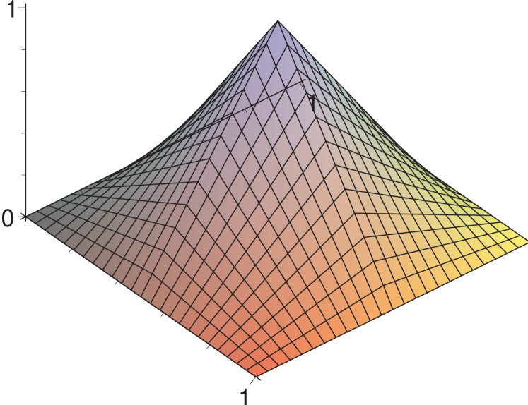
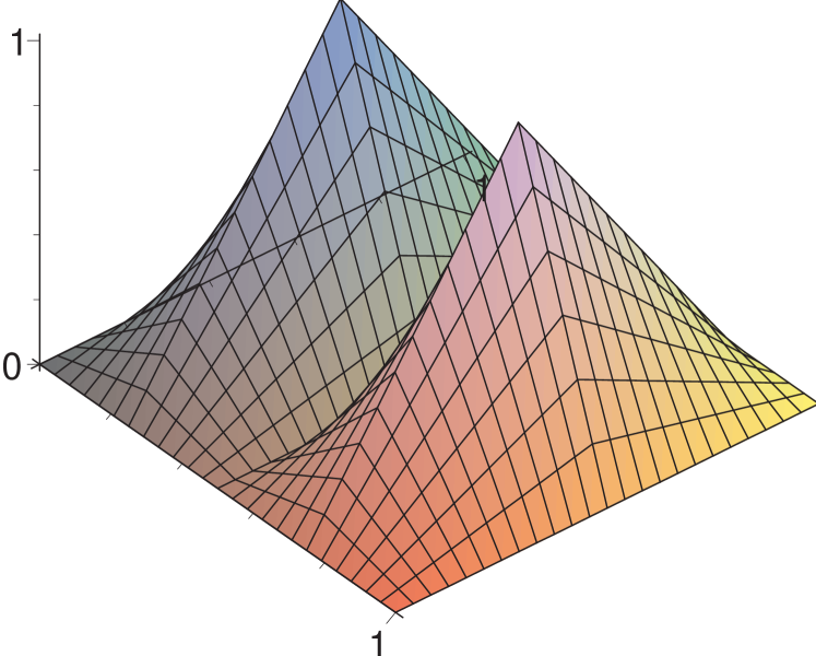
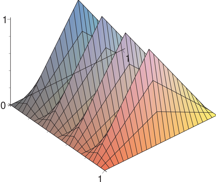
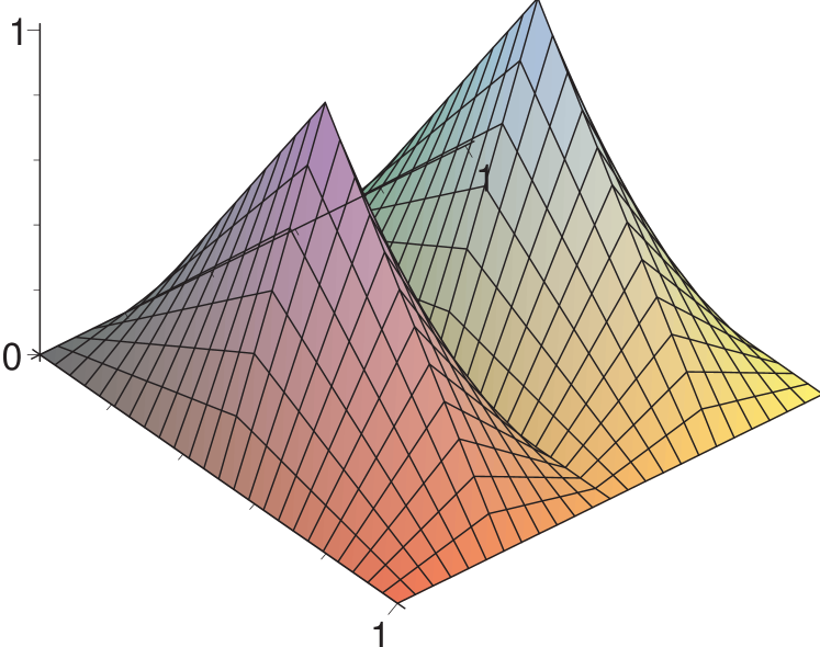
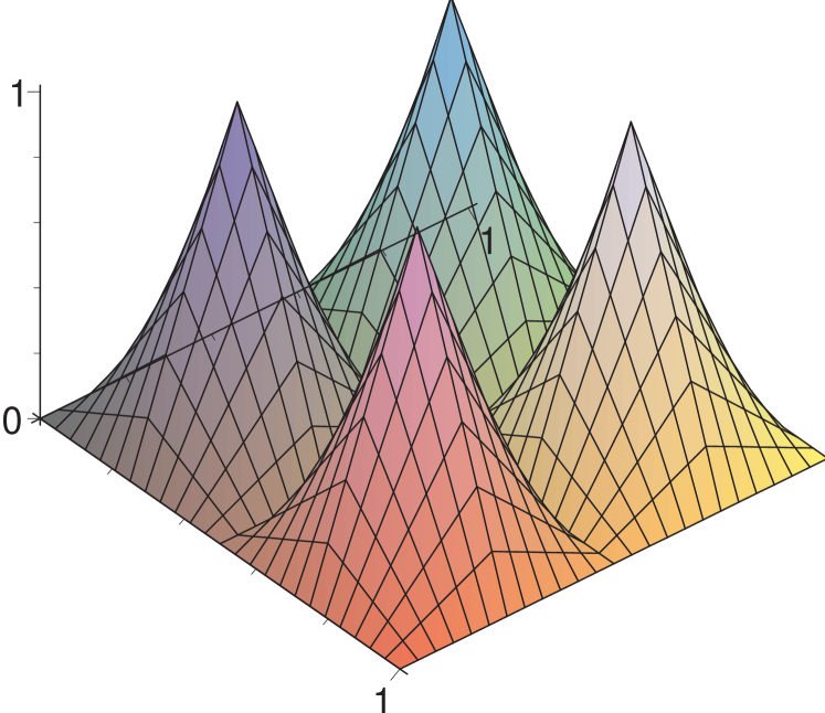
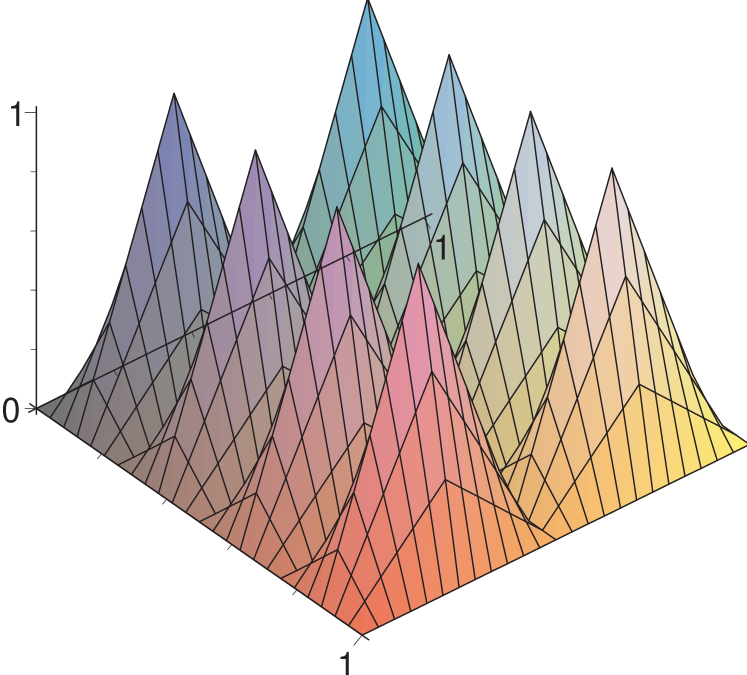
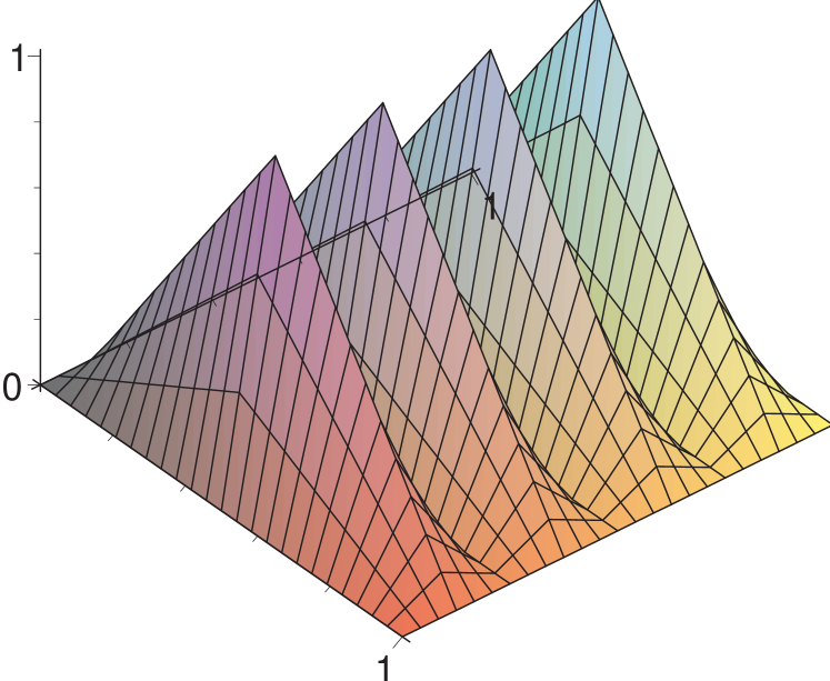
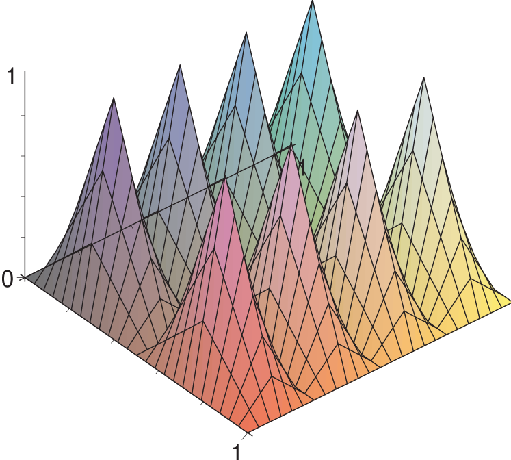
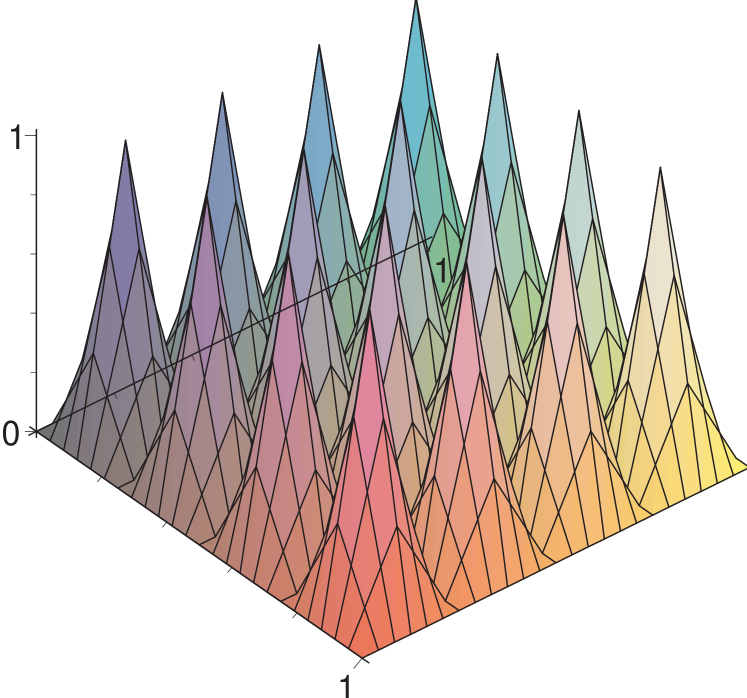
Here and later on, we need the $l_{1}$-norm $|\textrm{{\hbox{\boldmath$l$\unboldmath}}}|_{1}=\sum_{j=1}^{d}l_{j}$ and the maximum-norm $|\textrm{{\hbox{\boldmath$l$\unboldmath}}}|_{\infty}=\max_{1\leq j\leq d}l_{j}$ of multi-indices $l$. Figure 3 shows some 2-dimensional examples for the basis functions of the subspaces $W_{\textrm{{\hbox{\boldmath$l$\unboldmath}}}}$, which correspond to anisotropic sub-grids with mesh-width $h_{l_{j}}$ in dimension $j$ characterised by the multi-index $l$.

$W_{(1,1)^{T}}$

$W_{(2,1)^{T}}$

$W_{(3,1)^{T}}$

$\cdots$

$W_{(1,2)^{T}}$

$W_{(2,2)^{T}}$

$W_{(3,2)^{T}}$

$\cdots$

$W_{(1,3)^{T}}$

$W_{(2,3)^{T}}$

$W_{(3,3)^{T}}$

$\cdots$

$\vdots$

$\vdots$

$\vdots$

$\ddots$

Figure 3: Basis functions of the subspaces $W_{\textrm{{\hbox{\boldmath$l$\unboldmath}}}}$ for $|\textrm{{\hbox{\boldmath$l$\unboldmath}}}|_{\infty}\leq 3$ in two dimensions.

2.4 Sparse grids

Starting from the hierarchical representation of $V_{n}$ by the subspaces $W_{\textrm{{\hbox{\boldmath$l$\unboldmath}}}}$, we can now select those subspaces that contribute most to the overall solution of the full-grid interpolation (10). If the function we want to approximate meets certain smoothness conditions—the mixed second derivatives have to be bounded—this can be done a priori as we can derive bounds for the contributions of the different subspaces. We then obtain the sparse grid space

$$V_{n}^{(1)}\equiv\bigoplus_{|\textrm{{\hbox{\boldmath$l$\unboldmath}}}|_{1}\leq n+d-1}W_{\textrm{{\hbox{\boldmath$l$\unboldmath}}}}\,,$$ (11)

leaving out those subspaces from the full grid space $V_{n}$ with many basis functions of small support. (The exact choice of subspaces depends on the norm in which we measure the error; the result above is optimal for both the $L_{2}$ norm and the maximum norm.) Note that in the one-dimensional case, the sparse grid space equals the full grid space.

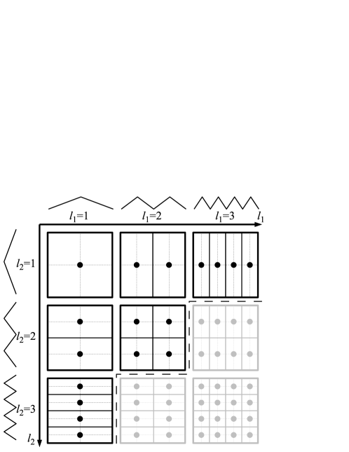
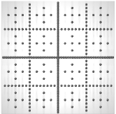
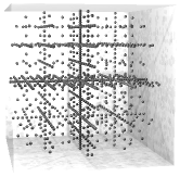
Figure 4 shows the selection of subspaces and the resulting sparse grid for $n=3$, i.e. the sparse grid space $V_{3}^{(1)}$. Compared to the full grid for the same discretisation level $n$ (the full grid space $V_{3}$ would also comprise the grey subspaces in Figure 4), this reduces the number of grid points (and therefore function evaluations and unknowns) significantly from ${\cal O}(h_{n}^{-d})={\cal O}(2^{nd})$ to ${\cal O}(h_{n}^{-1}(\log h_{n}^{-1})^{d-1})$ – whereas the asymptotic accuracy deteriorates only slightly from ${\cal O}(h_{n}^{2})$ to ${\cal O}(h_{n}^{2}(\log h_{n}^{-1})^{d-1})$, see Bungartz & Griebel (2004) for detailed derivations. Figure 5 shows sparse grids in two and three dimensions for level $n=6$ each.

$V^{(1)}_{3}$

Figure 4: The two-dimensional subspaces $W_{\textrm{{\hbox{\boldmath$l$\unboldmath}}}}$ up to $l=3$ ($h_{3}=1/8$) in each dimension. The optimal selection of subspaces (black) and the corresponding sparse grid on level $n=3$ for the sparse grid space $V_{3}^{(1)}$. The corresponding full grid of level 3 corresponds to the direct sum of all subspaces that are shown.

Figure 5: Sparse grids in two and three dimensions for level $n=6$.

Functions which do not meet the smoothness requirements or which show significantly differing characteristics (comprising steep regions as well as flat ones, e.g.) can be tackled as well, if adaptive refinement is used. The sparse grid structure (11) defines an a priori selection of grid points which is optimal if certain smoothness conditions are met and no further knowledge about the function in question is known or used. An adaptive (a posteriori) refinement can additionally select which grid points in a sparse grid structure should be refined next, due to local error estimation, e.g. To refine a grid point, often all $2d$ children in the hierarchical structure are added to the current grid, if they haven’t been created yet. Note that it usually has to be ensured that all missing parents have to be created, as algorithms working on sparse grids depend on traversals of the hierarchical tree of basis functions. If additional knowledge about the problem at hand is available, it can be used in the criterion for adaptive refinement, allowing to better adapt to problem specific characteristics.

2.5 Extension to functions that are non-zero on the boundary

Up until now we have only considered functions that are zero on the domain’s boundary $\delta\Omega$. To allow for non-zero values on the boundary, usually additional grid points located directly on $\delta\Omega$ are introduced. For example, the one-dimensional basis on level one, containing only $\varphi_{1,1}(x)$, is extended by two basis functions with level $0$ and indices $0$ and $1$ restricted to $\Omega$, namely $\varphi_{0,0}(x)$ and $\varphi_{0,1}(x)$. They are then extended to the $d$-dimensional case as before, with the exception that the new basis now contains basis functions on the modified level one with overlapping support.

Apparently, this approach results in many more grid points (and therefore expensive function evaluations) than before. This shows quite nicely that it is not sufficient to just consider the asymptotic behaviour: asymptotically, nothing changes, but for very high dimensionalities we are not able to even start to interpolate any more. In $d$ dimensions, the basis for the subspace $W_{\textrm{{\hbox{\boldmath$1$\unboldmath}}}}$ for example contains already $3^{d}$ basis functions, rather than a single one. Especially in settings where a very high accuracy close to the boundary is not required—which holds in our case—(or where an adaptive selection of grid points is used in any case), it can be advantageous to omit the grid points on the boundary, and instead modify the basis functions to extrapolate towards the boundary of the domain.

We modify the one-dimensional basis functions as follows: On level 1, we have only one degree of freedom; the best guess towards the boundary is to assume the same value, leading to a constant basis function. On all other levels, we extrapolate linearly towards the boundary, “folding up” the uttermost basis functions. All other basis functions remain unchanged, yielding

$$\varphi_{l,i}(x)\equiv\left\{\begin{array}[]{ll}1&\mbox{if }l=1\wedge i=1\,,\\[4.0pt] \varphi_{l,i}^{\rm left}(x)&\mbox{if }l>1\wedge i=1\,,\\[4.0pt] \varphi_{l,i}^{\rm right}(x)&\mbox{if }l>1\wedge i=2^{l}-1\,,\\[4.0pt] \varphi\left(x\cdot 2^{l}-i\right)&\mbox{else}\,,\end{array}\right.$$ (12)

with

$$\varphi_{l,i}^{\rm left}(x)\!\! \equiv \!\!\left\{\begin{array}[]{ll}2-2^{l}\cdot x{}{}{}{}{}&\mbox{if }x\in\left[0,\frac{1}{2^{l-1}}\right]\\ 0&\mbox{else}\end{array}\right\}\,,$$ (15)

$$\varphi_{l,i}^{\rm right}(x)\!\! \equiv \!\!\left\{\begin{array}[]{ll}2^{l}\cdot x+1-i&\mbox{if }x\in\left[1-\frac{1}{2^{l-1}},1\right]\\ 0&\mbox{else}\end{array}\right\}\,.$$ (18)

Examples of the modified one-dimensional basis functions are shown in Figure 6. The $d$-dimensional basis functions are obtained as before via a tensor product of the one-dimensional ones.

Figure 6: Modified one-dimensional basis functions $\varphi_{l,i}$: constant on level 1 and “folded up” if adjacent to the boundary on all other levels.

3 Interpolation of the WMAP likelihood surface

We now construct an interpolation of the WMAP log-likelihood, $\ln\mathcal{L}$, using sparse grids. In order to adapt the problem to our interpolation approach, we first use a 6-dimensional set of so-called normal parameters introduced in Sandvik et al. (2004), which are a transformation of the usual cosmological parameters such that the major axes of the Gaussian align with the coordinate axes. The logarithm of the likelihood is then well-approximated by a sum of one-dimensional parabolas in the different parameters, a fact that we will take advantage of by using the modified basis-functions described in (12). For this set of normal parameters, we obtain an accurate interpolation already for a comparably low refinement level. This is shown for the 6-dimensional model as well as for a 7-dimensional extension, using the running of the spectral index as an additional parameter.

However, as a subsequent step we demonstrate that the parameter transformation is not essential for obtaining a good interpolation. By investing more grid points, we obtain an accurate interpolation as well when using directly the 6- and 7-dimensional standard parameter set, which is usually used in cosmological parameter sampling. This approach shows the advantage of sparse grids of being rather generic. Furthermore, we are not restricted to the parameter range in which the transformation to normal parameters can be inverted.

3.1 Choice of basis functions

We use the modified basis functions as introduced in (12), which are well-suited for our problem. First, and as already indicated in Sec. 2, the region close to the domain’s boundary is less important in our setting than the centre of $\Omega$: We will centre the domain of interest roughly at the maximum of the log-likelihood function $\ln\mathcal{L}$ and determine the boundary such that it includes the region with $(\ln\mathcal{L}_{\rm max}-\ln\mathcal{L})\lesssim 25$, which we will refer to as the 25 log-likelihood region (see Sec. 3.3).

Towards the boundaries of our intervals, the likelihood is then effectively zero and thus no great accuracy is needed in these regions. Therefore, we do not want to spend too much work on $\delta\Omega$. Using the modified boundary functions, we extrapolate ($d$-linearly) towards $\delta\Omega$, see the discussion of the modified basis functions above.

Second, the modifications are especially well-suited if the function to interpolate can be separated into a sum of one-dimensional functions. Assume that the likelihood $\mathcal{L}$ was a perfect product of one-dimensional Gaussians,

$$\mathcal{L}(\textrm{{\hbox{\boldmath$x$\unboldmath}}})=c\cdot\operatorname{e}^{-a_{1}(x_{1}-\mu_{1})^{2}-\ldots-a_{d}(x_{d}-\mu_{d})^{2}}\,,$$ (19)

centred at $(\mu_{1},\ldots,\mu_{d})^{T}$. Then the interpolation of the log-likelihood $\ln\mathcal{L}$ reduces to $d$ one-dimensional problems,

$$\ln\mathcal{L}(\textrm{{\hbox{\boldmath$x$\unboldmath}}})=\ln c+\sum_{k=1}^{d}f_{k}(x_{k})\,,$$ (20)

with

$$f_{k}(x_{k})=-a_{k}(x_{k}-\mu_{k})^{2}\,,$$ (21)

separating into a constant term plus a sum of functions that are constant in all directions but one.

Keeping in mind that the one-dimensional basis function on level 1, $\varphi_{1,1}(x)$, is constant (cf. Figure 6), this simplifies the interpolation task. The $d$-dimensional basis function on level $1$, $\varphi_{\textrm{{\hbox{\boldmath$1$\unboldmath}}},\textrm{{\hbox{\boldmath$1$\unboldmath}}}}(\textrm{{\hbox{\boldmath$x$\unboldmath}}})$, serves as an offset. (Only if $(\mu_{1},\ldots,\mu_{d})^{T}$ is the centre of $\Omega$, $\alpha_{\textrm{{\hbox{\boldmath$1$\unboldmath}}},\textrm{{\hbox{\boldmath$1$\unboldmath}}}}\varphi_{\textrm{{\hbox{\boldmath$1$\unboldmath}}},\textrm{{\hbox{\boldmath$1$\unboldmath}}}}(\textrm{{\hbox{\boldmath$x$\unboldmath}}})$ exactly expresses $\ln c$.) Additionally, it is sufficient to spend only grid points on the main axes of the sparse grid (level 1 in all dimensions but one) to approximate the remaining one-dimensional contributions $f_{k}(x_{k})$ arbitrarily well:

$$u(\textrm{{\hbox{\boldmath$x$\unboldmath}}}) = \underbrace{\alpha_{\textrm{{\hbox{\boldmath$1$\unboldmath}}},\textrm{{\hbox{\boldmath$1$\unboldmath}}}}\varphi_{\textrm{{\hbox{\boldmath$1$\unboldmath}}},\textrm{{\hbox{\boldmath$1$\unboldmath}}}}(\textrm{{\hbox{\boldmath$x$\unboldmath}}})}_{\normalsize\ln c}$$ (22)

$$+\sum_{k=1}^{d}\underbrace{\left(\sum_{l_{k},i_{k}}\alpha_{\textrm{{\hbox{\boldmath$l$\unboldmath}}},\textrm{{\hbox{\boldmath$i$\unboldmath}}}}~{}\varphi_{l_{k},i_{k}}(x_{k})\!\!\!\!\!\prod_{1\leq j\leq d,j\neq k}\!\!\!\!\!\varphi_{1,1}(x_{j})\right)}_{\normalsize f_{k}(x_{k})}.$$

Of course, $\mathcal{L}$ is not a perfect product of one-dimensional Gaussians; grid points that do not lie on the sparse grid’s main axes account for the additional mixed (correlated) terms of $\ln\mathcal{L}$. Given that in sparse grids a large amount of points lie on the main axes, this mechanism works very well—the better, the less correlation between the different parameters exists.

In order to take as much advantage as possible of the effects described above, we introduce a parameter transformation in the following section, for which the new parameters are less correlated. However, the fact that the interpolation using the standard parameters—which have much stronger correlations—works as well, spending just more grid points, will show that the sparse grid approach does not depend on this argumentation: Sparse grids can make use of such properties but do not rely on them.

3.2 Normal parameters

The set of cosmological parameters describing the $\Lambda$CDM model consists of the Hubble constant, $h\equiv\frac{H_{0}}{100\,{\rm km}/(s{\rm Mpc})}$, the density parameter of vacuum energy, $\Omega_{\Lambda}$, the ones of baryons, $\Omega_{b}$, and of matter (baryonic + dark), $\Omega_{m}$, the optical depth to the last scattering surface, $\tau$, the scalar spectral index of the primordial power spectrum, $n_{s}$, and the scalar initial amplitude, $A_{s}$. We will refer to these parameters as cosmological parameters. For a more detailed description of the cosmological parameters, we refer to Coles & Lucchin (2002). In the literature, there have been several attempts to transforming these parameters into a set of parameters that mirror the various physical effects on the CMB power spectrum (Hu et al., 2001; Kosowsky et al., 2002). In Chu et al. (2003), a set of parameters is provided in which the likelihood-surface of the CMB is well approximated by a multivariate Gaussian with the major axes aligned with the coordinate axes. In this work, we use the parameters given by Sandvik et al. (2004), where the parameter set of Chu et al. (2003) is combined with the other parameter sets mentioned, in order to bring the major axes of the likelihood surface even closer to the coordinate axes. The new parameters are then $\{\Theta_{s},h_{2},h_{3},t,A_{*},Z\}$, which we refer to as normal parameters. When working with the latter, the logarithm of the likelihood is well-approximated by a sum of one-dimensional parabolas in the different parameters. The basis functions introduced above are therefore ideally adapted to this problem. In the following, we repeat the definitions of the normal parameters for convenience.

The first parameter of our set is the angle subtended by the acoustic scale

$$\Theta_{s}\equiv\frac{r_{s}(a_{{\rm ls}})}{D_{A}(a_{{\rm ls}})}\frac{180}{\pi}\,,$$ (23)

where the index ${{\rm ls}}$ denotes the time of last scattering, $D_{A}(a_{{\rm ls}})$ stands for the comoving angular diameter distance to the surface of last scattering (which we will come back to later), and $r_{s}(a_{{\rm ls}})$ is the comoving sound horizon at last scattering,

$$r_{s}(a_{{\rm ls}})\equiv\int_{0}^{t_{{\rm ls}}}\frac{c_{s}(t)}{a(t)}dt\,.$$ (24)

Here, $c_{s}(t)$ denotes the sound speed for the baryon-photon-fluid at time $t$, which is well approximated by

$$c_{s}(t)^{2}\approx\frac{1}{3}(1+3\frac{\rho_{b}}{\rho_{\gamma}})^{-1}\,,$$ (25)

with the index $b$ standing for baryons and the index $\gamma$ for photons. Using the Friedmann equations and ignoring the vacuum energy at last scattering, $r_{s}(a_{{\rm ls}})$ can be shown to be (Sandvik et al., 2004; Kosowsky et al., 2002)

$$r_{s}(a_{{\rm ls}})=\frac{2\sqrt{3}}{3H_{0}\sqrt{\Omega_{m}}}\sqrt{\frac{a_{{\rm ls}}}{R_{{\rm ls}}}}\ln\frac{\sqrt{1+R_{{\rm ls}}}+\sqrt{R_{{\rm ls}}+r_{{\rm ls}}R_{{\rm ls}}}}{1+\sqrt{r_{{\rm ls}}R_{{\rm ls}}}}\,,$$ (26)

where

$$R_{{\rm ls}} \equiv \frac{3\rho_{b}(a_{{\rm ls}})}{4\rho_{\gamma}(a_{{\rm ls}})}=30\,w_{b}\left(\frac{z_{{\rm ls}}}{10^{3}}\right)^{-1}\,,$$ (27)

$$r_{{\rm ls}} \equiv \frac{\rho_{r}(a_{{\rm ls}})}{\rho_{m}(A_{*})}=0.042\,w_{m}^{-1}\left(\frac{z_{{\rm ls}}}{10^{3}}\right)\,.$$ (28)

The index $r$ stands for radiation, i.e., $\,\rho_{r}$ consists of the sum of photon and neutrino energy densities, and the index $m$ is used for matter (baryons + dark matter). We define $w_{m}\equiv\Omega_{m}h^{2}$ in the same way as $w_{b}\equiv\Omega_{b}h^{2}$. The redshift at last scattering, $z_{{\rm ls}}$, is well approximated by (Hu et al., 2001)

$$z_{{\rm ls}} = 1048\,(1+0.00124\,w_{b}^{-0.738})(1+g_{1}w_{m}^{g_{2}})\,,$$ (29)

$$g_{1} \equiv 0.0783\,w_{b}^{-0.238}(1+39.5\,w_{b}^{0.763})^{-1}\,,$$ (30)

$$g_{2} \equiv 0.560\,(1+21.1w_{b}^{1.81})^{-1}\,.$$ (31)

As already mentioned, $D_{A}(a_{{\rm ls}})$ in (23) denotes the comoving angular diameter distance to the surface of last scattering and is given by

$$D_{A}(a_{{\rm ls}})=\frac{c}{H_{0}}\int_{a_{{\rm ls}}}^{1}\frac{1}{\sqrt{\Omega_{\Lambda}\tilde{a}^{4}+\Omega_{m}\,\tilde{a}+\Omega_{r}}}d\tilde{a}\,.$$ (32)

The second and third parameters in our set are the ratios of the second and the third peak to the first peak in the $C_{l}^{T}$ spectrum of the CMB (Hu et al., 2001), where the tilt-dependence is factored out (Page et al., 2003),

$$h_{2} \equiv 0.0264\,w_{b}^{-0.762}$$ (33)

$$\exp\left(-0.476\,[\ln(25.5\,w_{b}+1.84\,w_{m})]^{2}\right)\,,$$

$$h_{3} \equiv 2.17\left(1+\left(\frac{w_{b}}{0.044}\right)^{2}\right)^{-1}$$ (34)

$$w_{m}^{0.59}\left(1+1.63\left(1-\frac{w_{b}}{0.071}\right)w_{m}\right)^{-1}\,.$$

We use the tilt parameter given by Sandvik et al. (2004), which is a slightly modified version of the one in Chu et al. (2003) in order to minimise the correlation with $w_{b}$:

$$t\equiv\left(\frac{w_{b}}{0.024}\right)^{-0.5233}2^{n_{s}-1}\,.$$ (35)

The amplitude parameter is

$$A_{*}\equiv\frac{\tilde{A}_{s}}{2.95\times 10^{-9}}{\mathrm{e}}^{-2\tau}\left(\frac{k}{k_{p}}\right)^{n_{s}-1}w_{m}^{-0.568}\,,$$ (36)

where $k_{p}=0.05\mathrm{Mpc}^{-1}$ denotes the pivot point. The normalisation factor of $2.95\times 10^{-9}$ comes in because we use the scalar amplitude $\tilde{A}_{s}$ of CMBEASY, which is defined as the primordial power of the curvature fluctuations evaluated at the pivot point, $\tilde{A}_{s}\equiv\Delta_{R}^{2}(k_{p})$. It is related to the scalar amplitude $A_{s}$ of CMBFAST, which is used in Sandvik et al. (2004), by $A_{s}=\frac{\tilde{A}_{s}}{2.95\times 10^{-9}}$ (cf.  Verde et al., 2003). Finally, we use the physical damping due to the optical depth to last scattering as our last parameter:

$$Z\equiv{\mathrm{e}}^{-\tau}\,.$$ (37)

In order to construct the interpolation of the likelihood surface, we need the transformation that maps the normal parameters back onto cosmological parameters. The reason for this is the way we construct the interpolation: Our sparse grid algorithm chooses the normal parameters where it wants to refine the grid, which we then need to transform into cosmological parameters to run CMBEASY and the WMAP-likelihood code. Our technique of inverting the parameter transformation is presented in appendix A.

3.3 Generation of test set and choice of interpolation range

For choosing the parameter range in which to construct the interpolation, we have run MCMCs containing about 50,000 points at a temperature of $T=3$. That is, in the Metropolis algorithm we choose the transition probability $a(\textrm{{\hbox{\boldmath$x$\unboldmath}}},\textrm{{\hbox{\boldmath$y$\unboldmath}}})$ from a point $x$ in the chain to a new point $y$ to be $a(\textrm{{\hbox{\boldmath$x$\unboldmath}}},\textrm{{\hbox{\boldmath$y$\unboldmath}}})\equiv\min\left\{\left(\mathcal{L}(\textrm{{\hbox{\boldmath$y$\unboldmath}}})/\mathcal{L}(\textrm{{\hbox{\boldmath$x$\unboldmath}}})\right)^{\frac{1}{T}},1\right\}$. Using this transition probability with $T=1$ results in the usual Metropolis algorithm, whereas choosing $T=3$ allows us to explore a larger parameter range than with the regular algorithm. These chains covered a region reaching out to about 25 log-likelihoods around the peak.

The optical depth to the last scattering surface, $\tau$, which can be determined from the CMB polarization, is not well-constrained by the WMAP polarization data due to their low signal-to-noise ratio. Therefore, when running the MCMCs at $T=3$, we had to restrict $\tau$ to the physically meaningful range $\tau\geq 0$. This restriction corresponds to $Z\leq 1$ for the normal parameters. In the case of the normal parameters in 7 dimensions, we had to additionally restrict the intervals to $h_{2}\leq 0.52$ and $h_{3}\geq 0.38$, which is the range in which the parameter transformation is invertible. Furthermore, we chose to restrict our set of points to be within the 25 log-likelihood region around the peak.

In order to roughly centre our intervals at the maximum of the log-likelihood function, we have determined the latter using a few runs of a simple simplex search. The interval boundaries were then defined as the box centred at the maximum which contains all points of the above-described chains. Note that it is not important for the accuracy of the interpolation that the intervals are well-centred at the maximum. Note further that we have used this set of points as a test set for comparing our interpolation with the real log-likelihood.

3.4 Results

Figure 7: Absolute error of the interpolation with respect to the real log-likelihood in 6 dimensions for an interpolation with a sparse grid of level 5 (top panel) and of level 6 (bottom panel) for normal parameters.

Figure 8: Absolute error of the interpolation with respect to the real log-likelihood in 7 dimensions for an interpolation with a sparse grid of level 6 (top panel) and of level 7 (bottom panel) for normal parameters.

We have interpolated the log-likelihood of the WMAP 5 year data in the 6-dimensional normal parameter space described in Sec. 3.2. The same has been done for a 7-dimensional model, in which we have chosen the running of the spectral index of the primordial power spectrum, $\alpha$, as an additional parameter. Constructing the interpolation can be parallelised to an arbitrary degree, according to the available computational resources.

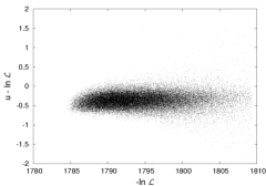
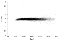
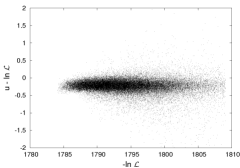
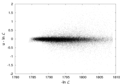
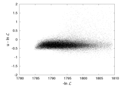
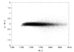
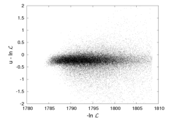
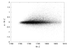
For the 6-dimensional model, we plot the absolute error of the log-likelihood, $(u-\ln\mathcal{L})$, against the negative WMAP log-likelihood, $(-\ln\mathcal{L})$, for the points in the test set in Figure 7. We have used an interpolation on a sparse grid of level $n=5$ (consisting of 2561 grid points) in the top panel, and of level $n=6$ (consisting of 10625 grid points) in the bottom panel. One clearly sees the improvement in accuracy when increasing the grid level from $n=5$ to $n=6$. Figure 8 shows the same plot for the 7-dimensional model, for grid level $n=6$ (18943 grid points) in the top panel and $n=7$ (78079 grid points) in the bottom panel. We again see the improvement in accuracy with increasing refinement level. However, the additional parameter $\alpha$ is quite strongly correlated with many of the other parameters, whereas the correlations between the normal parameters in 6 dimensions are reduced to a minimum. We therefore have to increase the grid level by one in 7 dimensions, in order to obtain results comparable to the 6-dimensional ones. In both figures, we note a systematic negative offset of the interpolation with respect to the real function, which becomes less severe for the higher refinement levels. This offset is due to the fact that we construct a $d$-linear interpolant of a convex function, which systematically lies below the function. This could be easily coped with by adding a small offset to $\alpha_{\textrm{{\hbox{\boldmath$1$\unboldmath}}},\textrm{{\hbox{\boldmath$1$\unboldmath}}}}$ after the interpolation, or, even better, by using piecewise polynomial instead of the piecewise linear basis functions. We leave the usage of piecewise polynomial basis functions, which promise to be well-adapted to the log-likelihood, for future work.

Note that we have restricted the plot range to [-2,2], because only 0.1 per cent or less of the points lie outside this range. Almost all of these points lie in the corners of $\Omega$ due to relatively strongly correlated parameters. These are the regions in parameter space where the 25 log-likelihood range around the peak extends to the interval boundaries. Due to the extrapolation we use close to the boundaries (cf. the end of Sec. 2), we obtain relatively large uncertainties in those regions, which do not affect the one-dimensional projections of the likelihood function, though. The uncertainties can be further reduced, spending (adaptively) more grid points in those regions, see also the discussion about adaptivity in Sec. 3.5.

For the 6-dimensional interpolation with a sparse grid of level 6, 2.5 per cent of the test points have an absolute error $>0.25$ in the log-likelihood, and 0.03 per cent of the test points have an absolute error $>1$. In 7 dimensions and for refinement level 7, the corresponding numbers are 9 per cent and 0.5 per cent, respectively. This is a higher level of accuracy as reached by Pico (Fendt & Wandelt, 2007), for which about 90 per cent of the points in a region reaching out to 25 log-likelihoods around the peak have been calculated with an absolute error below 0.25. However, we note that these numbers for Pico are valid for a 9-dimensional parameter space, whereas we work in 6- and 7-dimensional spaces and leave the extension to higher-dimensional models to future work. But we also note that in all settings where a systematic offset in the interpolation error can be observed, it is sufficient to reduce the offset to improve our results significantly, in particular for interpolations on lower levels (see, e.g., the scatterplot for the 6-dimensional model and grid level 5, Figure 7).

We have projected both the interpolation and the WMAP likelihood function using MCMCs of about 150,000 points, and compare the results for the 7-dimensional model for grid level $n=6$ in Figure 9. We reproduce the projected one-dimensional likelihood curves almost perfectly. The results for the 6-dimensional model for grid level $n=5$ are very similar to the 7-dimensional ones. Note that we obtain these excellent results for the 6-dimensional model using only 2561 grid points. The visual comparison of our results with the projected one-dimensional likelihoods obtained by CosmoNet (Auld et al., 2007, 2008) shows that we reproduce the original curves with a higher accuracy than the latter. Note also that our interpolation is constructed in a rather wide region, encompassing about 25 log-likelihoods around the peak, whereas in Auld et al. (2008) the region in which $\ln\mathcal{L}$ was fitted covers only $4\sigma$ around the peak for the combined likelihood of CMB and LSS. This corresponds to a region of about 8 log-likelihoods around the peak for the combined likelihood, and even less when using only the CMB likelihood.

Figure 9: Comparison of the one-dimensional projections of the 7-dimensional WMAP 5 year likelihood (solid) and its interpolation (dashed) using a sparse grid of level $n=6$ (consisting of 18943 grid points) for normal parameters. The curves match almost perfectly.

Consider now the interpolation of the WMAP likelihood surface using directly the standard parameters, which are used by default when doing cosmological parameter sampling with the MCMC driver from CMBEASY (Doran & Müller, 2004): $\{w_{m},w_{b},h,\tau,n_{s},\ln(10^{10}A_{s})-2\tau\}$, to which we again add $\alpha$ as an additional parameter in the 7-dimensional case. Working with these parameters has the advantage that we do not have to restrict ourselves to the parameter range in which the parameter transformation is invertible. However, the problem is now less adapted to our choice of basis functions, due to the stronger correlations between the different parameters. We therefore pay the price of having to increase the grid level by one in this case in order to reach an accuracy as good as before. We show the absolute error of the log-likelihood, $(u-\ln\mathcal{L})$, against the negative WMAP log-likelihood, $(-\ln\mathcal{L})$, for the 6-dimensional model for grid level $n=6$ (10625 points) and $n=7$ (40193 points) in Figure 10, and for the 7-dimensional one for $n=7$ (87079 points) and $n=8$ (297727 points) in Figure 11. For the 6-dimensional (7-dimensional) interpolation with a sparse grid of level $n=7$ ($n=8$), the fraction of test points with absolute error $>0.25$ in the log-likelihood is 6 per cent (20 per cent), and 0.5 per cent (2.5 per cent) for an absolute error $>1$. Again, the one-dimensional projections of the 6-dimensional case for level $n=6$ and of the 7-dimensional case for level $n=7$ are very similar to the ones in Figure 9, and are thus not shown.

Figure 10: Absolute error of the interpolation with respect to the real log-likelihood in 6 dimensions for an interpolation with a sparse grid of level 6 (top panel) and of level 7 (bottom panel) for standard parameters.

Figure 11: Absolute error of the interpolation with respect to the real log-likelihood in 7 dimensions for an interpolation with a sparse grid of level 7 (top panel) and of level 8 (bottom panel) for standard parameters.

We have tested the evaluation time of our interpolation by evaluating a sparse grid interpolant of level 6 in 6 dimensions for 2,000,000 points randomly chosen from within $\Omega$. On a conventional desktop computer (Intel chipset, 2.8 GHz), this took about $92\,\mu s$ per point, including the random generation of the point. In 7 dimensions on the same level we have twice as many grid points and one dimension more, which doubles the evaluation time to $189\,\mu s$. For CosmoNet and Pico, the evaluation of a 6-dimensional model is specified to take about $10\,\mu s$ and $250\,\mu s$, respectively (Auld et al., 2008). Note that we do not know on which hardware the evaluation times of CosmoNet and Pico have been measured, which makes a comparison hardly possible. Note further that our code to evaluate a sparse grid function is not optimised for fast evaluation times and that there is still room for improvement. In any case, for all of these codes the bottleneck in cosmological parameter sampling is now the MCMC algorithm itself rather than the evaluation of the likelihood, at least with the MCMC driver used in this work (Doran & Müller, 2004).

Note that in 7 dimensions, we need significantly more grid points than in 6 dimensions, since the additional parameter $\alpha$ strongly correlates with the other parameters, and we thus need to increase the grid level by one to obtain good results. As the storage requirements are rather low, this mainly increases the number of evaluations that are needed for constructing the sparse grid interpolation. As already stated before, though, the construction of the interpolation can be parallelised to an arbitrary degree, according to available computational resources, so that this should not be an issue. To store the interpolant for a regular sparse grid in $d$ dimensions for level $l$ with $N$ grid points, we would only need $N$ doubles for the coefficients and two integers to remember both $d$ and $l$, leading to $(N+1)\cdot 8$ Bytes. For adaptively refined sparse grids, we additionally have to store at least which grid points have been refined, requiring slightly more storage. For current hardware architectures, the size of the memory is therefore not a limiting factor for our application.

We have shown in this section, that the interpolation of the log-likelihood with regular sparse grids provides excellent and competitive results in both 6 and 7 dimensions, even when interpolating in the rather wide range covering about 25 log-likelihoods around the peak. The memory requirements to store the sparse grid are rather low and the evaluation times are very fast. We have demonstrated that the one-dimensional projections of the interpolants match the original ones almost perfectly, and that the scatterplots of the errors exhibit only a small fraction of grid points with higher errors. For standard parameters, more grid points have to be spent to obtain the same accuracy than for normal parameters, as the latter ones correlate less. In the next section, we will therefore focus on an adaptive extension of the method used so far to further reduce the number of grid points that are required.

3.5 Improvements with adaptive sparse grids

As it has already been mentioned, the log-likelihood is not a perfect sum of one-dimensional functions. The different parameters contribute differently to $\mathcal{L}$ and correlate more or less with each other. It is therefore reasonable, especially when using the standard parameters which correlate more, to employ adaptivity, spending more grid points in critical regions and less grid points elsewhere. In this section, we demonstrate the utility of adaptivity by showing some first results as a proof of concept. As they can clearly be improved further, we leave a thorough study of adaptive sparse grids for the interpolation of $\ln\mathcal{L}$ to future work. We start by specifying how to refine, we formally derive a suitable criterion that can be used to specify where to refine as well as to measure the quality of an interpolation, and we finally provide results that show how adaptivity can improve the interpolation obtained for regular sparse grids.

Employing adaptivity, one can attempt to either obtain better results fixing roughly the number of grid points used, or to achieve a similar accuracy using less grid points. In the following, we show results for the former, tackling the 7-dimensional example using the standard parameters on level 7 with 78079 grid points presented above. We start with a regular sparse grid of some low level and refine grid points, creating all $2d$ children in the hierarchical structure (if possible) each, until the grid size exceeds 78000 grid points. In settings where the contributions of the dimensionalities differ significantly, it can be useful to start with level 2 to allow dimensional adaptivity, neglecting unimportant dimensions; here, the grid points on low levels will be created in any case, so we can start with a sparse grid on level 5, e.g., to save on the number of adaptive steps.

Choosing a suitable refinement criterion, it can be determined whether to refine in a broad way (close to regular sparse grids) or in a more greedy way in the sparse grid’s hierarchical tree structure. It is reasonable to take the surpluses of the grid points into account as they contain the local information about the functions, i.e., if the function has a high gradient locally. Furthermore, they decay quickly with increasing level-sum in the convergent phase. The mere surplus-based criterion, refining the grid points with the highest absolute value of the surplus first, is known to tend to minimise the $L_{2}$-norm of the error. As we do not spend grid points on the domain’s boundary, and as we are extrapolating towards the boundary, the biggest surpluses per level can be found for the modified basis functions which are adjacent to the boundary. A mere surplus-based criterion will therefore only refine towards the boundary. This reduces the error especially for sampling points with a high error in the scatterplots, as they are located towards the boundary of the domain.

In the following, we theoretically derive a refinement criterion which is better suited to our problem than the purely surplus-based one. In order to maximise the information our interpolation contains about the real likelihood, we attempt to minimise the Kullback-Leibler distance $d_{KL}$ between the interpolation and the likelihood function,

$$d_{KL} \equiv \int d^{d}x\,\mathcal{L}(\textrm{{\hbox{\boldmath$x$\unboldmath}}})\ln\frac{\mathcal{L}(\textrm{{\hbox{\boldmath$x$\unboldmath}}})}{\exp(u(\textrm{{\hbox{\boldmath$x$\unboldmath}}}))}$$ (38)

$$= \int d^{d}x\,\mathcal{L}(\textrm{{\hbox{\boldmath$x$\unboldmath}}})\left(\ln\mathcal{L}(\textrm{{\hbox{\boldmath$x$\unboldmath}}})-u(\textrm{{\hbox{\boldmath$x$\unboldmath}}})\right)\,,$$

which is defined for two normalised probability distributions $\mathcal{L}$ and $\exp(u)$. Let us now derive the refinement criterion we obtain from minimising $d_{KL}$. Assume that we have already computed an interpolation $u(\textrm{{\hbox{\boldmath$x$\unboldmath}}})$ with $N$ grid points, then the Kullback-Leibler distance $d_{KL}$ when evaluating the function at an additional point $\textrm{{\hbox{\boldmath$x$\unboldmath}}}_{N+1}$ is changed by

$$\left|d_{KL}^{\rm new}-d_{KL}^{\rm old}\right|\!\!\! = \!\!\!\bigg{|}\int d^{d}x\,\mathcal{L}(\textrm{{\hbox{\boldmath$x$\unboldmath}}})\bigg{[}\ln\mathcal{L}(\textrm{{\hbox{\boldmath$x$\unboldmath}}})-u^{\rm new}(\textrm{{\hbox{\boldmath$x$\unboldmath}}}).$$ (39)

$$\!\!\!-\ln\mathcal{L}(\textrm{{\hbox{\boldmath$x$\unboldmath}}})+u^{\rm old}(\textrm{{\hbox{\boldmath$x$\unboldmath}}})\bigg{]}\bigg{|}$$

$$= \!\!\!\left|\int d^{d}x\,\mathcal{L}(\textrm{{\hbox{\boldmath$x$\unboldmath}}})\left[u^{\rm old}(\textrm{{\hbox{\boldmath$x$\unboldmath}}})-u^{\rm new}(\textrm{{\hbox{\boldmath$x$\unboldmath}}})\right]\right|$$

$$= \!\!\!\left|\int d^{d}x\,\mathcal{L}(\textrm{{\hbox{\boldmath$x$\unboldmath}}})\left[\sum_{i=1}^{N}\alpha_{i}\varphi_{i}(\textrm{{\hbox{\boldmath$x$\unboldmath}}})-\sum_{i=1}^{N+1}\alpha_{i}\varphi_{i}(\textrm{{\hbox{\boldmath$x$\unboldmath}}})\right]\right|$$

$$= \!\!\!\left|\int d^{d}x\,\mathcal{L}(\textrm{{\hbox{\boldmath$x$\unboldmath}}})\left[\alpha_{N+1}\varphi_{N+1}(\textrm{{\hbox{\boldmath$x$\unboldmath}}})\right]\right|\,.$$

If we refine the interpolation around the grid point that contributed most to the Kullback-Leibler distance, we can hope to converge towards the minimum of $d_{KL}$ fastest. In order to obtain a suitable refinement criterion, we have to simplify the formula in (39) considerably. We thus assume the likelihood $\mathcal{L}(\textrm{{\hbox{\boldmath$x$\unboldmath}}})$ as well as the basis function $\varphi_{N+1}(\textrm{{\hbox{\boldmath$x$\unboldmath}}})$ to be locally constant on $\varphi_{N+1}$’s support, obtaining

$$\left|d_{KL}^{\rm new}-d_{KL}^{\rm old}\right|\sim V_{N+1}\mathcal{L}(\textrm{{\hbox{\boldmath$x$\unboldmath}}}_{N+1})\,|\alpha_{N+1}|\,,$$ (40)

where $V_{N+1}$ is the volume covered by the basis function $\varphi_{N+1}$ (i.e. its support), and we have used $\varphi_{N+1}(\textrm{{\hbox{\boldmath$x$\unboldmath}}}_{N+1})=1$.

With (40), we have derived an estimation of the contribution of a basis function to $d_{KL}$, which is a reasonable refinement criterion in our setting. In addition to the surplus of the grid point, $|\alpha_{N+1}|$, it takes into account the value of the likelihood $\mathcal{L}(\textrm{{\hbox{\boldmath$x$\unboldmath}}}_{N+1})$ at the grid point, and the volume of the basis function $V_{N+1}$. The likelihood takes care of the fact that we would like to be more accurate where the likelihood is higher. The regions of very low likelihood are less interesting for us—the likelihood being already very close to zero beyond a difference of about 20 log-likelihoods. The volume factor, on the other hand, prevents the interpolation to refine too deeply (to very high grid levels) locally in the parameter space. However, since this usually only takes effect after several refinement steps, and as we have restricted the number of grid points, we choose not to include the volume factor but rather to refine several points at the same time, which addresses this issue in an alternative way, and which will be discussed later on. We further choose to introduce a temperature $T$ again, which allows us to weight the likelihood with respect to the surplus and thus to influence how much to refine close to the maximum. The refinement criterion we used in this study is thus

$$\left(\frac{\mathcal{L}(\textrm{{\hbox{\boldmath$x$\unboldmath}}}_{\textrm{{\hbox{\boldmath$l$\unboldmath}}},\textrm{{\hbox{\boldmath$i$\unboldmath}}}})}{\mathcal{L}_{\rm{max}}}\right)^{1/T}\,|\alpha_{\textrm{{\hbox{\boldmath$l$\unboldmath}}},\textrm{{\hbox{\boldmath$i$\unboldmath}}}}|\,,$$ (41)

where we have divided the likelihood by its peak value, $\mathcal{L}_{\rm{max}}$, (which we have already obtained determining the interpolation domain) because the WMAP code returns the log-likelihood only up to a constant offset, so that we do not know the correct normalisation of $\mathcal{L}$. For $T=1$, refinement takes place only very close to the maximum as $\mathcal{L}$ decays quickly; a temperature of $T=6$ showed to provide good results within the whole domain of interest.

Refining only one grid point per refinement step often causes adaptivity to get stuck in a single, special characteristic of the function. Interpolating $\ln\mathcal{L}$ with our choice of basis functions, all grid points are likely to be created only in the direction where the log-likelihood decays fastest, or around one of the local dips we will address later on. Refining more than one grid point at the same time helps to circumvent such effects, resulting in a broader refinement scheme.

The Kullback-Leibler distance $d_{KL}$ can also be used to measure the quality of our interpolation: The distance between the real likelihood and or interpolation should be as small as possible. However, as we have already mentioned above, we do not know the normalisation of the WMAP likelihood function. Therefore, $d_{KL}$ is not necessarily positive and thus looses its property of being a useful measure of the ‘closeness’ of the two functions. We thus use a slightly modified version,

$${\widehat{d}}_{KL}\equiv\int d^{d}x\,\mathcal{L}(\textrm{{\hbox{\boldmath$x$\unboldmath}}})|\ln\mathcal{L}(\textrm{{\hbox{\boldmath$x$\unboldmath}}})-u(\textrm{{\hbox{\boldmath$x$\unboldmath}}})|\,,$$ (42)

as a measure of the quality of our interpolation, instead of the actual Kullback-Leibler distance. It can be easily calculated from an MCMC with $T=1$ obtained for $\mathcal{L}$, by simply averaging the absolute errors $|\ln\mathcal{L}(\textrm{{\hbox{\boldmath$x$\unboldmath}}}_{i})-u(\textrm{{\hbox{\boldmath$x$\unboldmath}}}_{i})|$ over all points in the chains. Furthermore, we quote this value averaged over a chain of $T=3$ (exploiting the interpolation domain better), which corresponds to $\int d^{d}x\,\mathcal{L}(\textrm{{\hbox{\boldmath$x$\unboldmath}}})^{\frac{1}{T}}|\ln\mathcal{L}(\textrm{{\hbox{\boldmath$x$\unboldmath}}})-u(\textrm{{\hbox{\boldmath$x$\unboldmath}}})|$.

Figure 12 shows the scatterplot for an adaptively refined sparse grid in 7 dimensions. Starting from a regular grid of level 5, we refined 100 grid points each according to the refinement criterion (41) with $T=6$.

Figure 12: Absolute error of the interpolation with respect to the real log-likelihood in 7 dimensions for an interpolation with an adaptively refined sparse grid for standard parameters.

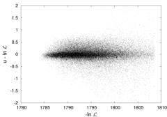
Needing only about as much grid points (78551) as for the regular sparse grid of level 7, Tab. 1 shows that we obtain results which are close to those of a regular sparse grid of level 8 with almost 4 times as many grid points. We provide the Mean Squared Error (MSE) as well as ${\widehat{d}}_{KL}$ for both $T=1$ and $T=3$ chains for regular sparse grids of level 7 and 8, and for the adaptively refined case. We also quote how many points exhibit an absolute error larger than 1 or 0.25 for the $T=3$ chains. We do not show the histograms of the adaptively refined model, as the histograms for both the regular grid on level 8 and the adaptively refined one, are very close to the histograms for normal parameters in 7 dimensions shown in Figure 9.

	err $>1$, T=3	err $>0.25$, T=3	MSE, T=1	MSE, T=3	$\widehat{d}_{KL}$, T=1	$\widehat{d}_{KL}$, T=3
level 7	4.2%	50.5%	0.087	0.532	0.256	0.354
level 8	2.3%	19.3%	0.017	0.210	0.091	0.193
adaptive	1.8%	23.6%	0.027	0.202	0.110	0.204

Table 1: Comparison of errors of regular sparse grids of level 7 and level 8, respectively, and an adaptively refined sparse grid using approximately as many grid points as contained in the regular grid of level 7. Shown are the number of points with an absolute error larger than 1 or 0.25 in the $T=3$ chains, the MSE for chains of $T=1$ and $T=3$, and ${\widehat{d}_{KL}}$, which denotes the absolute value of the error averaged over chains of $T=1$ and $T=3$.

We would like to mention, that, due to numerical problems, the current version of CMBEASY produces local, unphysical and sometimes rather high dips. This problem is already known and will be corrected in the next release. For stochastic approaches, this is not a big problem, though: The dips are local and just cause some noisy evaluations. But it poses a problem for numerical approaches if a grid point hits a dip. Then it can happen, that spending more grid points can even deteriorate the results. For our regular grid in 6 dimensions using the standard parameters, e.g., increasing the level from 7 to 8 caused a higher overall error on the chain-data used for the histograms, as especially two new basis functions close to the peak caused an error of up to 12 of the log-likelihood for all evaluations affected by those basis functions.

Fortunately, dips can be detected automatically due to the hierarchical structure of the sparse grid and the smoothness of $\ln\mathcal{L}$, using a criterion that is once more based on the surpluses. Furthermore, it is not a severe problem when using adaptivity, as adaptivity localises the effects of the dips automatically. One just has to take care not to spend too much grid points to compensate for the dips.

The first adaptive results are promising, but there is still room for a lot of improvement. Even better refinement criteria than those used so far could be employed. Using not only piecewise linear functions, but rather piecewise polynomials, and applying adaptivity in both the mesh-width and the polynomial degree is very promising; especially the extrapolation properties towards the boundary would be improved, and less grid points would be needed to obtain the same accuracies.

4 Conclusions

In this work, we have explored the utility of interpolating the WMAP log-likelihood surface using sparse grids. We demonstrated that the results are excellent and competitive to other approaches regarding speed and accuracy, and we discussed advantages over fitting the likelihood surface with polynomials (Fendt & Wandelt, 2007; Sandvik et al., 2004) or neural networks (Auld et al., 2008):

The interpolation based on sparse grids converges towards the exact function in the limit of the grid level going to infinity. We can therefore reach an arbitrary accuracy by simply increasing the amount of work we spend. In the case of a polynomial fit, this is not guaranteed since increasing the polynomial degree runs the risk of becoming unstable.

In order to construct the sparse grid interpolation, we do not need to sample a set of training points using MCMCs beforehand, since the sampling points are determined by the sparse grid structure which is given a priori. Once we have chosen the volume of interest, the time for constructing the interpolation is dominated by the evaluation of the likelihood function at the grid points. We do not need additional training time as for neural networks (Auld et al., 2008), for example. Constructing the interpolation can thus be done almost arbitrarily in parallel, only limited by the computational resources that are available.

The sparse grid technique is rather general and not restricted to certain classes of functions. In particular, the choice of sampling points and basis functions is not tailored to a single problem as for neural networks, where the topology of the network has to be chosen problem-specifically (often in a heuristic way). The sparse grid interpolation technique as well as our extensions can therefore be readily applied to other problems in astrophysics and cosmology, and will be useful in further tasks, where an accurate interpolation of a function is needed.

The excellent performance of the sparse grid interpolation can be further improved, leaving future research to do: It can be applied to models with more than seven parameters by spending more computational effort. Further modification of the basis functions, for example allowing for a piecewise polynomial interpolation, promises better convergence rates and higher accuracies. Adaptive refinement schemes, which take into account the characteristics of the interpolated function, can be used to further increase the accuracy of the interpolation, as we have already demonstrated for a first example in this work.

Chapter

Appendix A Inversion of the parameter transformation

In the following, we present a technique of inverting the parameter transformation of Sec. 3.2 to compute the cosmological parameters given the normal parameters. The normal parameter $h_{2}$ in terms of cosmological parameters is given by

$$h_{2}(w_{m},w_{b})\!\! = \!\!0.0264\,w_{b}^{-0.762}$$ (43)

$$\!\!\exp\left(-0.476\left[\ln(25.5\,w_{b}+1.84\,w_{m})\right]^{2}\right)\,.$$

We solve this equation for $w_{m}$ as a first step:

$$w_{m}(h_{2},w_{b})\!\!\!\! = \!\!\!\!\bigg{(}\exp\left\{\pm\left[-\frac{1}{0.476}\ln\left(\frac{h_{2}}{0.0264}\,w_{b}^{0.762}\right)\right]^{1/2}\right\}$$ (44)

$$\!\!\!\!-25.5\,w_{b}\bigg{)}\frac{1}{1.84}\,.$$

Inconveniently, there exist two different solutions for $w_{m}(h_{2},w_{b})$, which complicates the inversion. We now substitute $w_{m}$ in $h_{3}(w_{m},w_{b})$ (34) for (44) and thus obtain $h_{3}(h_{2},w_{b})$, which, of course, has two solutions as well. An example of the two branches of $h_{3}(h_{2},w_{b})$ for $h_{2}=0.45$ is depicted in Fig. 13.

Figure 13: The two branches of $h_{3}$ versus $w_{b}$ for $h_{2}=0.45$.

We can compute the critical point where only one solution exists using the condition

$$-\frac{1}{0.476}\ln\left(\frac{h_{2}}{0.0264}\,w_{b}^{0.762}\right)=0\,,$$ (45)

as can be seen from (44). This condition gives us the following formulae for the parameter values at the critical point:

$$w_{b,{\rm crit}}(h_{2}) = \left(\frac{0.0264}{h_{2}}\right)^{1/0.762}\,,$$ (46)

$$w_{m,{\rm crit}}(h_{2}) = \left(1-25.5\,w_{b,{\rm crit}}\right)\frac{1}{1.84}\,,$$ (47)

$$h_{3,{\rm crit}}(h_{2}) = 2.17\left(1+\left(\frac{w_{b,{\rm crit}}}{0.044}\right)^{2}\right)^{-1}w_{m,{\rm crit}}^{0.59}$$ (48)

$$\left(1+1.63\left(1-\frac{w_{b,{\rm crit}}}{0.071}\right)w_{m,{\rm crit}}\right)^{-1}\,.$$

The two parameters $h_{2}$ and $h_{3}$ can now be inverted to $w_{m}$ and $w_{b}$. For a given $h_{2}$, we express $h_{3}$ in terms of $h_{2}$ and $w_{b}$, as described above. We then use $h_{3,{\rm crit}}(h_{2})$ to choose the upper branch of $h_{3}(h_{2},w_{b})$ if our given $h_{3}$ is bigger than $h_{3,{\rm crit}}(h_{2})$, and the lower branch if it is smaller. Using the respective branch of $h_{3}(h_{2},w_{b})$, we search numerically in $w_{b}$ until $h_{3}(h_{2},w_{b})$ matches the given $h_{3}$. Substituting that value of $w_{b}$ into equation (44), we readily obtain the value for $w_{m}$.

Now it is straightforward to compute the values for $n_{s}$ and $A_{s}$ from $t$ and $A_{*}$. To obtain $h$ from $\Theta_{s}$, we follow the procedure suggested by Kosowsky et al. (2002), expressing $\Theta_{s}$ in terms of $h$ in terms of $h$ and then searching in $h$ numerically until $\Theta_{s}(h)$ matches the given value of $\Theta_{s}$.

References

- Auld et al. (2008) Auld T., Bridges M., Hobson M. P., 2008, MNRAS, 387, 1575
- Auld et al. (2007) Auld T., Bridges M., Hobson M. P., Gull S. F., 2007, MNRAS, 376, L11
- Bellman (1961) Bellman R., 1961, Adaptive Control Processes: A Guided Tour. Princeton University Press
- Bungartz & Griebel (2004) Bungartz H.-J., Griebel M., 2004, Acta Numerica, 13, 147
- Bungartz et al. (2008) Bungartz H.-J., Pflüger D., Zimmer S., 2008, in Bock H., Kostina E., Hoang X., Rannacher R., eds, Modelling, Simulation and Optimization of Complex Processes, Proceedings of the High Performance Scientific Computing 2006, Hanoi, Vietnam Adaptive sparse grid techniques for data mining. Springer, pp 121–130
- Chu et al. (2003) Chu M., Kaplinghat M., Knox L., 2003, ApJ, 596, 725
- Coles & Lucchin (2002) Coles P., Lucchin F., 2002, Cosmology: The Origin and Evolution of Cosmic Structure, Second Edition
- Doran (2005) Doran M., 2005, Journal of Cosmology and Astro-Particle Physics, 10, 11
- Doran & Müller (2004) Doran M., Müller C. M., 2004, Journal of Cosmology and Astro-Particle Physics, 9, 3
- Fendt & Wandelt (2007) Fendt W. A., Wandelt B. D., 2007, arXiv:0712.0194
- Ganapathysubramanian & Zabaras (2007) Ganapathysubramanian B., Zabaras N., 2007, J. Comput. Phys., 225, 652
- Garcke (2006) Garcke J., 2006, in ICML ’06: Proceedings of the 23rd international conference on Machine learning Regression with the optimised combination technique. ACM Press, New York, NY, USA, pp 321–328
- Garcke et al. (2001) Garcke J., Griebel M., Thess M., 2001, Computing, 67, 225
- Garcke & Hegland (2009) Garcke J., Hegland M., 2009, Computing, 84, 1
- Habib et al. (2007) Habib S., Heitmann K., Higdon D., Nakhleh C., Williams B., 2007, Phys. Rev. D, 76, 083503
- Holtz (2008) Holtz M., 2008, Dissertation, Institut für Numerische Simulation, Universität Bonn
- Hu et al. (2001) Hu W., Fukugita M., Zaldarriaga M., Tegmark M., 2001, ApJ, 549, 669
- Jimenez et al. (2004) Jimenez R., Verde L., Peiris H., Kosowsky A., 2004, Phys. Rev. D, 70, 023005
- Kaplinghat et al. (2002) Kaplinghat M., Knox L., Skordis C., 2002, ApJ, 578, 665
- Klimke et al. (2006) Klimke A., Nunes R., Wohlmuth B., 2006, Internat. J. Uncertain. Fuzziness Knowledge-Based Systems, 14, 561
- Kosowsky et al. (2002) Kosowsky A., Milosavljevic M., Jimenez R., 2002, Phys. Rev. D, 66, 063007
- Lewis et al. (2000) Lewis A., Challinor A., Lasenby A., 2000, ApJ, 538, 473
- Page et al. (2003) Page L., et al., 2003, ApJS, 148, 233
- Reisinger & Wittum (2007) Reisinger C., Wittum G., 2007, SIAM J. Scientific Computing, 29, 440
- Sandvik et al. (2004) Sandvik H. B., Tegmark M., Wang X., Zaldarriaga M., 2004, Phys. Rev. D, 69, 063005
- Seljak & Zaldarriaga (1996) Seljak U., Zaldarriaga M., 1996, ApJ, 469, 437
- Tauber (2000) Tauber J. A., 2000, Astrophysical Letters Communications, 37, 145
- Temlyakov (1993) Temlyakov V. N., 1993, Approximation of Periodic Functions. Nova Science Publishers
- Verde et al. (2003) Verde L., et al., 2003, ApJS, 148, 195
- von Petersdorff & Schwab (2006) von Petersdorff T., Schwab C., 2006, Appl. Math., 51, 145
- Widmer et al. (2008) Widmer G., Hiptmair R., Schwab C., 2008, Journal of Computational Physics, 227, 6071
- Zenger (1991) Zenger C., 1991, in Hackbusch W., ed., Parallel Algorithms for Partial Differential Equations Vol. 31 of Notes on Numerical Fluid Mechanics, Sparse grids. Vieweg, pp 241–251
Chapter \thechapter