Towards a high precision calculation for the pion-nucleus scattering lengths

Abstract

We calculate the leading isospin conserving few-nucleon contributions to pion scattering on ²H, ³He, and ⁴He. We demonstrate that the strong contributions to the pion-nucleus scattering lengths can be controlled theoretically to an accuracy of a few percent for isoscalar nuclei and of 10% for isovector nuclei. In particular, we find the $\pi$-³He scattering length to be $(62\pm 4\pm 7)\times 10^{-3}m_{\pi}^{-1}$ where the uncertainties are due to ambiguities in the $\pi$-N scattering lengths and few-nucleon effects, respectively. To establish this accuracy we need to identify a suitable power counting for pion-nucleus scattering. For this purpose we study the dependence of the two-nucleon contributions to the scattering length on the binding energy of ²H. Furthermore, we investigate the relative size of the leading two-, three-, and four-nucleon contributions. For the numerical evaluation of the pertinent integrals, a Monte Carlo method suitable for momentum space is devised. Our results show that in general the power counting suggested by Weinberg is capable to properly predict the relative importance of $N$-nucleon operators, however, it fails to capture the relative strength of $N$- and $\left(N+1\right)$-nucleon operators, where we find a suppression by a factor of 5 compared to the predicted factor of 50. The relevance for the extraction of the isoscalar $\pi$-N scattering length from pionic ²H and ⁴He is discussed. As a side result, we show that the calculation of the $\pi$-²H scattering length is already beyond the range of applicability of heavy pion effective field theory.

1 Introduction

The probably most fundamental quantities characterizing pion scattering off nucleons are the pion-nucleon ($\pi$-N) scattering lengths. Obviously being low energy observables, one should be able to understand their size based on the effective field theory (EFT) of Quantum Chromodynamics (QCD), namely Chiral Perturbation Theory (ChPT). In fact, the impact of symmetries on these quantities is known for a long time Weinberg:1966kf ; Tomozawa:1966jm (for a recent review see Ref. Bernard:2007zu ), but for a quantitative analysis of high accuracy it is of utmost importance to understand now in detail the higher order corrections, either isospin symmetric ones or isospin symmetry violating (IV) ones, based on ChPT, for they point directly at QCD dynamics.

Despite an on-going effort to learn more on the scattering lengths experimentally, they are still not very accurately known Gasser:2007zt . This is especially true for the isoscalar scattering length which is so small, that a high control over various other, normally neglected effects, like IV, is necessary for a reliable extraction of $a^{(+)}$ from experiment. On the theoretical side important progress for IV $\pi$-N scattering is reported in Refs. Hoferichter:2009gn ; Hoferichter:2009ez ; Gasser:2002am . A first extraction of the leading charge symmetry breaking (a special case of IV interactions) $\pi$-N scattering amplitude is reported in Refs. vanKolck:2000ip ; Bolton:2009rq ; Filin:2009yh based on an analysis of the recent observation of the IV forward–backward asymmetry in $pn\to d\pi^{0}$ Opper:2003sb .

The most promising way to get experimental access to the $\pi$-N scattering lengths is the investigation of pionic atoms, the simplest system being pionic hydrogen. Many efforts have been undertaken to measure energy shift and width of this system, allowing for an extraction of the isoscalar and isovector $\pi$-N scattering lengths $a^{(+)}$ and $a^{(-)}$ assuming that isospin symmetry is exact up to standard Coulomb interactions Schroder:1999uq ; Schroder:2001rc .

In principle, it appears to be possible to extract both the isoscalar and the isovector scattering length from pionic hydrogen data, for the measurement provides two independent observables, namely the level shift compared to the QED value induced by the strong interaction as well as the width, where the transition $\pi^{-}p\to\pi^{0}n$ gives a significant, known contribution. However, in order to improve the extraction accuracy and to better control systematics, an additional source of $a^{(+)}$ is desireable. In this context, it is important to study more complex systems, like pionic deuterium, ³He, or ⁴He, for the wave functions for those nuclei can be calculated with high accuracy. It is easy to see that the pion-nucleus scattering length $a_{\pi-A}$ can be written as

$$a_{\pi-A} = \left(\frac{1+\frac{m_{\pi}}{m_{N}}}{1+\frac{m_{\pi}}{A\,m_{N}}}\right)\left(Aa^{\left(+\right)}-Q_{\pi}\,a^{\left(-\right)}2T_{3}\right)$$ (3)

$$\hskip 85.35826pt+\mbox{few-nucleon corrections}$$

$$\hskip 85.35826pt+\mbox{IV corrections}$$

Here, $A$ denotes the mass number of the nucleus, $T_{3}$ the third component of its isospin, $m_{\pi}$ and $Q_{\pi}$ the mass and charge of the pion and $m_{N}$ the nucleon mass. We will not further discuss the IV corrections here, instead we refer to Refs. Meissner:2005ne ; Gasser:2007zt for a review on the current status of IV in pion-nucleus scattering. Especially, the isospin $T=0$ nuclei ²H and ⁴He yield important new information since contributions from $a^{(-)}$ are suppressed and the contribution of $a^{(+)}$ is more prominent. From Eq. (3) it becomes clear that an understanding of these more complex systems requires to understand with a high accuracy the few-nucleon contributions to the scattering length. For $\pi$-²H scattering they have been studied for decades within potential multiple scattering theory, see e.g. Refs.Baru:1997xf ; Ericson:2000md ; Doring:2004kt and references therein. A first attempt to calculate few-body effects systematically and model-independently, i.e. within ChPT, was done by Weinberg Weinberg:1992yk . He proposed to organize the transition operator as an expansion in $m_{\pi}/\Lambda$ with $\Lambda$ being the chiral symmetry breaking scale of the order of 1 GeV. This transition operator was then convoluted in Ref. Weinberg:1992yk with phenomenological models for the nucleon-nucleon (NN) interaction. This work has been refined in Ref. Beane:1997yg . The explicit calculations showed that part of the few-nucleon corrections seem to be suppressed. Maybe even more troublesome for the extraction of $\pi$-N scattering lengths is the observation that the few-nucleon corrections were somewhat larger than naive dimensional analysis predicted. Such issues were addressed in Beane:2002wk . Here a refined power counting, the so-called $Q$–counting, was proposed that takes the small binding energy of ²H explicitly into account. Assuming that typical momenta of the nucleons are given by the binding momentum $\gamma=\sqrt{E_{d}m_{N}}$, with $E_{d}$ denoting the deuteron binding energy, it was found that the estimated magnitudes of various few-body corrections changed drastically and thus the series needed to be reorganized compared to the original power counting used in Weinberg:1992yk . Obviously, it is important to investigate the validity of this assumption, before extending the approach to even more complex systems or towards higher orders.

As mentioned above, the second issue of the first calculations of two-nucleon corrections to $\pi$-²H scattering is the relatively large size of the leading few-nucleon terms. Recently, higher order contributions to this class of diagrams have been investigated in Ref. Beane:2002wk and Refs. Lensky:2006wd ; Baru:2007wf . Especially, the results of the latter references indicate that the small scale $\gamma$ does not play a role in the higher order terms studied in Refs. Lensky:2006wd ; Baru:2007wf . It is however not clear at this point, whether the hierarchy of two-, three- and four-nucleon contributions is as expected by the power counting. An understanding of the systematics of such higher order corrections is mandatory when analyzing data on ³He and ⁴He.

In this paper, we study the presumably leading two-, three- and four-nucleon contributions explicitly. In Sec. 2, we will discuss the implications of using the different power countings in more detail. In Sec. 3, we repeat the well-known expressions for two-nucleon operators, derive a complete set of leading three-nucleon operators and give expressions for the probably most relevant example of a four-nucleon operator. The contribution to the scattering length based on these expressions requires the evaluation of high dimensional integrals involving the operators and few-nucleon wave functions. Such a problem will also appear in other applications. Therefore, we explain our numerical method for such calculations in detail in Sec. 4. In Sec. 5, we turn to ²H and study the dependence of the leading two-nucleon contributions on the binding energy based on an unphysically over- or underbound ²H. The results will shed light on the validity of $Q$–counting. We then introduce the input into our calculations for the required few-nucleon wave functions in more detail in Sec. 6. This is a prerequisite for our further studies. Sec. 7 is devoted to ³He where the scattering length of $\pi$-³He system is calculated. For the first time, we give explicit results for the contribution of three-nucleon corrections to pion-nucleus scattering. Finally, in Sec. 8, we estimate four-nucleon contributions to $\pi$-⁴He scattering based on an explicit calculation. We then summarize our findings and conclude in Sec. 9. More technical aspects of this work are deferred to the appendices.

2 Power-counting schemes for pion-nucleus scattering

The central goal of this work is to provide the calculations necessary to extract the isoscalar scattering length from data on the pion-nucleus scattering length. The basis for this is a reliable power counting which allows one to identify the relevant operators and provides a framework to estimate the diagrams not included. To reach maximal predictive power we include in each channel all diagrams that contribute up to one order lower than the contribution of the leading, unknown counter term. Especially the estimate of higher order operators requires some care. We here estimate the contributions from higher order operators, not calculated explicitly, by two methods:

• We demonstrate that all $N$-nucleon diagrams included can be organized in a series in powers of some parameter $\chi$. Thus, a calculation performed up to order $\chi^{n}$ is expected to have an uncertainty of order $\chi^{(n+1)}$.

• Using a set of wave functions generated for regulators varying over a large range of values, we investigate quantitatively the regulator dependence of the various matrix elements. This regulator dependence should be absorbed into a pertinent counter term. Therefore, we get access to the possible counter term contribution.

As we will see, for isoscalar nuclei both methods give consistent results supporting our claim that the scattering of pions off isoscalar targets at threshold can be calculated with an uncertainty of the order of 5 % of the leading two-nucleon contributions: $1\times 10^{-3}\ m_{\pi}^{-1}$ for $\pi$-²H and $2\times 10^{-3}\ m_{\pi}^{-1}$ for $\pi$-⁴He scattering. For isovector nuclei the contribution of the leading contact term is estimated via scaling of the leading isoscalar contribution. This allows us to estimate the accuracy of the calculation for $\pi$-³He scattering to be of the order of 10%.

It should also be stressed that up to now we are not able to identify a power counting that allows one to relate operators with different numbers of active nucleons, say one-nucleon with two- or three-nucleon operators. However, although we do not quantitatively understand the reasons for successive suppression of operators with an increasing number of active nucleons, the suppression observed numerically is quantitatively sufficiently large to allow for controlled results. In addition, it turns out that the successive suppression observed between $N$- and $\left(N+1\right)$-nucleon operators is the same for $N=1,\ 2,\ 3$, which is important for controlled uncertainty estimates. We also demonstrate that it is indeed possible to estimate reliably the relative importance of various $N$-nucleon operators.

What we need to carry out this program is a reliable power counting. There are two scales relevant for pion-nucleus scattering at threshold, namely the pion mass, $m_{\pi}$, and the nucleus binding momentum, $\gamma$, which may either be evaluated via

$$\gamma=\sqrt{2\mu\epsilon}\ ,$$ (4)

with $\mu$ for the reduced mass of a single nucleon with respect to the remainder and $\epsilon$ for the binding energy with respect to the first break-up channel, or via

$$\tilde{\gamma}=\sqrt{2m_{N}(E/A)}\ ,$$ (5)

with $(E/A)$ for the binding energy per nucleon. For the nuclei of relevance here — ²H, ³He, and ⁴He — both formulas give similar answers, namely $46$ and $46$ MeV, $82$ and $69$ MeV, and $167$ and $115$ MeV for $\gamma$ and $\tilde{\gamma}$ for the three nuclei in order. In the following we will therefore only use the quantity $\gamma$ for the binding momentum.

Let $q$ denote some generic momentum. There are two different power-counting schemes proposed for pion-nucleus scattering at threshold. These differ in how $q$ is treated relative to $m_{\pi}$ and $\gamma$. In Ref. Weinberg:1992yk , referred to as Weinberg counting, the assignment

$$q\sim m_{\pi}$$ (6)

is proposed while in Ref. Beane:2002wk , in the following called $Q$–counting,

$$q\sim\gamma\ll m_{\pi}$$ (7)

is used. In  Beane:2002wk the authors argue that the latter assignment is to be preferred, since, for $\pi$-²H scattering, $i)$ it naturally explains why the contribution of Diagram $(a)$ of Fig. 1 is more than an order of magnitude larger than those of $(b)$ and $(c)$; $ii)$ it quantitatively explains the magnitude of the contribution of the diagram of Fig. 2; and $iii)$ it quantitatively explains the contribution of the boost correction — this term emerges as a recoil correction to the leading isoscalar $\pi$-N scattering amplitude.

As in the $\pi$N sector, chiral symmetry enforces that operators that are odd under the exchange of the external pions — isovector operators — appear with at least one derivative acting on the pion field, while those that are even — isoscalar — have at least two derivatives or one insertion of the quark mass matrix. As a consequence, isoscalar operators are one order in $m_{\pi}/m_{N}$ suppressed compared to their isovector counter parts. This is another argument in favour of using isoscalar targets to get high accuracy information on the $\pi$-N scattering lengths: since the contribution of the leading order counter term sets the limit for the accuracy for the extraction of the $\pi$-N scattering lengths, the analysis of the scattering off isovector nuclei provides values for the scattering lengths about an order of magnitude less accurate.

The pertinent few-body corrections can now be classified in terms of $q$ and $m_{\pi}$. Because of the arguments above, the leading isoscalar 4N$\pi\pi$ counter term contributes to the $\pi$-²H scattering length at order $(m_{\pi}/m_{N})^{2}$, where for simplicity we identified the chiral symmetry breaking scale with the nucleon mass, while the leading two-nucleon correction — Diagram $(a)$ of Fig. 1 — scales as $(m_{\pi}/q)^{2}$. Explicit calculation gives that the leading two-nucleon diagram contributes about 20$\times 10^{-3}\,m_{\pi}^{-1}$ to the $\pi$-²H scattering length. Thus in the Weinberg scheme we estimate about 1$\times 10^{-3}\,m_{\pi}^{-1}$ for the leading counter term contribution while in $Q$–counting the leading counter term is expected to contribute only 0.1$\times 10^{-3}\,m_{\pi}^{-1}$, since the leading two-nucleon term benefits from an enhancement of order $(m_{\pi}/q)^{2}\simeq(m_{\pi}/\gamma)^{2}$ in $Q$–counting. Thus again, if we aim at a reliable estimate of the accuracy of the calculations performed we need to understand which one of the power-counting schemes describes the hierarchy of diagrams for pion-nucleus scattering at threshold. This will be done in Sec. 5.1.

It turns out that Weinberg and $Q$–counting predict a very different binding energy dependence of ratios of few-body corrections. These relations can be tested empirically: the NN potential at leading order of the chiral expansion comprises 1$\pi$–exchange and two counter terms. One of them can be adjusted such that any given (physical or unphysical) deuteron binding energy can be reproduced. This has been done to investigate the binding energy dependence of the relevant ratios of few-nucleon contributions. The main conclusion of Sec. 5.2 will be that the binding energy dependence of these ratios is in accordance with the prediction from Weinberg — up to logarithmic corrections — and in strong disagreement to the prediction from $Q$–counting.

In addition to providing some explanation for the apparent suppression of $a_{\pi-A}^{(1bc)}$ vs. $a_{\pi-A}^{(1a)}$, in Ref. Beane:2002wk it was argued that boosted $\pi$-N amplitudes give a significant contribution (number $iii)$ in the list given above), in discrepancy to what is expected from Weinberg counting. On the other hand, since the corresponding operator is proportional to the square of the nucleon momentum, this would imply an observable effect of the nucleon kinetic energy inside the deuteron, which is in conflict with general properties of field theories. In Ref. Baru:2007wf both problems were solved: once the $\Delta$–isobar is included as an explicit degree of freedom, simultaneously the residual boost contribution becomes sufficiently small to be in line with Weinberg counting and appears at an order where there is also a counter term.

Finally, we analyze the contribution of the triple scattering diagram of Fig. 2 in Sec. 5.3. In Weinberg counting this diagram is estimated to contribute only at order $(m_{\pi}/m_{N})^{2}$ relative to the leading two-nucleon operator. On the other hand numerical studies revealed that its actual value exceeds this estimate by about an order of magnitude. In Sec. 5.3 we will demonstrate that this enhancement is not due to the smallness of the deuteron binding energy, contrary to the claim in Ref. Beane:2002wk , but due to an integrable singularity in the corresponding expression that produces an enhancement by a factor of $\pi^{2}$. In view of this, also item $ii)$ of the list that was used to argue in favour of $Q$–counting does not apply anymore.

We are led to conclude that Weinberg counting gives a more reliable power counting scheme than $Q$–counting.

With these remarks, we now want to look at the possible few-nucleon contributions in more detail.

3 Few-nucleon contributions

Our main concern here are the few-nucleon corrections. For an evaluation of such contributions, expectation values of the basic pion–few-nucleon ($\pi$-$A$) amplitudes with the few-nucleon wave functions need to be calculated. Such wave functions can be obtained using standard methods to solve the few-nucleon Schrödinger equation based on nucleon-nucleon (NN) interactions Carlson:1997qn . Whereas in the first attempts to understand such contributions, wave functions based on phenomenological NN interactions were used Weinberg:1992yk ; Beane:1997yg , it is by now standard to also employ wave functions generated with nuclear interactions based on ChPT. The basic idea is to use naive dimensional analysis for a potential, which is then used to solve a Schrödinger equation Weinberg:1990rz ; Weinberg:1991um . Several groups have developed NN interactions based on this approach Ordonez:1995rz ; Entem:2003ft ; Epelbaum:2004fk and also three- (3N) and four-nucleon (4N) interactions have been formulated vanKolck:1994yi ; Bernard:2007sp and employed Epelbaum:2005pn , see also Ref. Epelbaum:2008ga for a recent review. Obviously, employing chiral interactions is preferable to calculate the pion-nucleus scattering length since nuclear interactions and $\pi$-$A$ amplitudes will be consistent.

In this work, we will present results on both kinds of interactions. We still show results based on phenomenological interactions, namely AV18  Wiringa:1994wb , Nijmegen 93  Stoks:1994wp , and CD-Bonn  Machleidt:2000ge . For ³He and ⁴He, we augment the nuclear Hamiltonian by a 3N interaction, so that the binding energies of these nuclei are reasonably well reproduced Nogga:2001cz . These results may serve as benchmark and might give indications on the size of the model-dependence of older calculations. We also employ wave functions based on chiral nuclear interactions between the leading order (LO, order 0 in the chiral expansion) and next-to-next-to-leading order (N²LO, order 3 in the chiral expansion).

Chiral interactions require a regularization scheme in order to obtain a well-defined Schrödinger equation. Most realizations use a momentum cutoff of the order of 500 MeV to this aim. For the leading order, at least when restricting oneself to $S$-wave interactions, it is possible to obtain fits for a much larger range of cutoffs Nogga:2005hy . These attempts have triggered a controversy in the community Hammer:2006qj . It should be noted that an inconsistency becomes apparent for large cutoffs, when higher order NN interactions are used Epelbaum:2009sd . Here, we use a wide range of cutoffs only for LO interactions, so that also this inconsistency does not apply. This allows us to use results for a wide range of cutoffs to estimate the size of leading counter terms. Parameter sets for the $S$-wave contact interactions are given in Tables 3, 4, and 5. Since these calculations are by no means high precision ones, we have neglected the minor contribution of higher partial waves in this case.

For the higher order chiral forces, we have employed order 2 (NLO) and order 3 (N²LO) ones of Ref. Epelbaum:2004fk . In the N²LO case, we added, as required by power counting, 3N forces, which were tuned to reproduce the ³He binding energy and N-²H scattering lengths.

Since we restrict ourselves to leading, tree-level $\pi$-$A$ operators, we may derive them using Feynman diagrams as done below. The reduction from four-dimensional quantities to three-dimensional ones can be easily performed using the on-shell energies of nucleons and pions. The pertinent integrals involving the wave functions and operators will be given below since their form depends on the number of nucleons involved.

3.1 Leading two-nucleon contributions

\psfrag{k}{\scriptsize${k}_{\pi}$}\psfrag{k'}{\scriptsize${k}_{\pi}^{\,\prime}$}\psfrag{q}{\scriptsize${q}$}\psfrag{q0}{\scriptsize${\tilde{q}}$}\psfrag{q1}{\scriptsize${\tilde{q}}$}\psfrag{q2}{\scriptsize${-\tilde{q}}$}\psfrag{a}{\scriptsize$a$}\psfrag{b}{\scriptsize$b$}\psfrag{c}{\scriptsize$c$}\psfrag{d}{\scriptsize$d$}\psfrag{e}{\scriptsize$e$}\psfrag{tau1}{\scriptsize$\tau_{1}$}\psfrag{tau2}{\scriptsize$\tau_{2}$}\psfrag{tau1d}{\scriptsize$\tau_{1}^{d}$}\psfrag{tau2e}{\scriptsize$\tau_{2}^{e}$}\includegraphics[scale={0.55}]{figures/2N-ops_psfrag.eps}

Figure 1: Leading two-nucleon contributions to $\pi$-$A$ scattering.

The leading two-nucleon contributions are known for many years Weinberg:1992yk ; Beane:1997yg ; Beane:2002wk . In the following, we call the numerically most important contribution, depicted in Fig. 1(a), “Coulombian” because of its ${1\over{\vec{q}}^{2}}$ pion propagator. The explicit expression for the amplitude is

$$i\mathcal{M}^{\left(\mbox{\scriptsize\ref{fig:2N-ops}a}\right)} = i\frac{m_{\pi}^{2}}{4f_{\pi}^{4}\;\vec{q}^{\,2}}\big{\{}2\delta^{ab}\left(\vec{\tau}_{1}\cdot\vec{\tau}_{2}\right)-\tau_{1}^{b}\tau_{2}^{a}-\tau_{1}^{a}\tau_{2}^{b}\big{\}}$$ (8)

where $\vec{q}$ is the momentum transfer between the nucleons, the $\vec{\tau}_{i}$ are usual Pauli matrices acting in the isospin space of nucleon $i$ and $f_{\pi}$ the pion decay constant. Throughout this work, we employ $f_{\pi}=92.4$ MeV. The small latin letters refer to isospin indices of the pions as given in the figure.

The amplitudes of Figs. 1(b) and 1(c) are individually dependent on the parametrization of the pion field. The sum of both, however, is independent of this choice as it should. Therefore, we will only show results for the sum of both contributions for which the amplitude reads

$$i\mathcal{M}^{\left(\mbox{\scriptsize\ref{fig:2N-ops}b+\ref{fig:2N-ops}c}\right)} = -i\frac{g_{A}^{2}m_{\pi}^{2}}{4f_{\pi}^{4}}\frac{1}{\left(\vec{q}^{\,2}+m_{\pi}^{2}\right)^{2}}\left(\vec{\sigma}_{1}\cdot\vec{q}\right)\left(\vec{\sigma}_{2}\cdot\vec{q}\right)$$ (9)

$$\quad\times\big{\{}\delta^{ab}\left(\vec{\tau}_{1}\cdot\vec{\tau}_{2}\right)-\left(\tau_{1}^{a}\tau_{2}^{b}+\tau_{1}^{b}\tau_{2}^{a}\right)\big{\}}.$$

Here, we additionally encounter $\vec{\sigma}_{i}$, the Pauli matrices acting in the spin space of nucleon $i$. Since the propagators contain an additional pion mass, we will refer to this contribution as “non-Coulombian”.

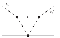
Figure 2: Triple scattering two-nucleon diagram.

In addition, in Ref. Beane:2002wk , the diagram shown in Fig. 2 was identified as numerically important, although in Weinberg counting it appears only at order N²LO as compared to the leading order diagrams of Fig. 1. This observation was taken as a support for the modified power counting, $Q$–counting, as discussed in the previous section. As we will show in section 5.3, a part of this amplitude is indeed enhanced, however, not parametrically but as a consequence of the special topology of the diagram. Therefore we also include this triple scattering diagram, although this is not supported by a power counting yet. Straightforward evaluation of its most dominant part gives

$$i\mathcal{M}^{\left(\mbox{\scriptsize\ref{fig:2N-triple}}\right)} = -2i\left(\frac{m_{\pi}}{2f_{\pi}^{2}}\right)^{3}\frac{1}{8|\vec{q}|}$$ (10)

$$\times\left\{\tau_{1}^{b}\tau_{2}^{a}+\tau_{1}^{a}\tau_{2}^{b}+\frac{i}{2}\epsilon^{abe}\left(\tau_{1}^{e}+\tau_{2}^{e}\right)\right\}.$$

For a discussion of the full expression for the amplitude we refer to Sec. 5.3. It is important to note that, although the triple scattering diagram is enhanced compared to what is expected from dimensional analysis, this enhancement is not sufficient to fully overcome the parametric suppression as provided by chiral symmetry. Comparing the double scattering contribution, Eq. (8), to the triple scattering contribution, Eq. (10), we still find a relative suppression of order

$$m_{\pi}^{2}/(16f_{\pi}^{2})\sim 0.14\ ,$$

which is close to the ratio found from the exact evaluation of the matrix elements. Thus, there is a suppression by an order of magnitude between the two contributions. We conjecture that the related diagram with four $\pi$N interactions will be suppressed by yet another order of magnitude and is therefore irrelevant for this study. Note, however, in case of $K$-nucleus scattering a resummation of the multiple scattering series is unavoidable Kamalov:2000iy ; Meissner:2006gx ; Baru:2009tx . Also in Ref. Baru:2009tx , it was argued that a resummation needs to be done including nucleon recoil effects in the propagators, for the nucleon recoil in multiple scattering diagrams induces potentially important corrections of the order of $\sqrt{m_{K}/m_{N}}$, with $m_{K}$ being the kaon mass, as compared to the static contributions.

As was argued above, all diagrams that contribute to lower orders than the first counter term should be included in this study. In addition to the diagrams discussed so far, there are potentially also those that are enhanced due to the presence of either two-nucleon or $\pi$NN–cuts. Moreover, there are also contributions from the $\Delta$–isobar. The effect of the $\pi$NN–cuts was discussed in detail in Ref. Baru:2004kw , see also Ref. Lensky:2005hb for a related discussion. It was shown in Ref. Baru:2004kw that, although formally enhanced, the contributions of the $\pi$NN–cuts to the $\pi$-²H scattering length nearly vanish as a result of a cancellation of different two-nucleon diagrams enforced by the Pauli principle. The same argument also applies to the scattering off ⁴He. In Ref. Lensky:2006wd and Baru:2007wf it was shown that diagrams with an NN–cut, often called dispersive terms , and those with an intermediate $\Delta$ start to contribute at the same order. Although individually sizable, the two groups of diagrams cancel each other nearly exactly. This cancellation should also appear in heavier nuclei whenever pions get scattered off an isoscalar NN pair. The analogous diagrams for isovector NN pairs were not studied yet, however, their contribution is intimately connected to the reaction $pp\to pp\pi^{0}$. The total cross section near threshold in this pion production channel, which is the relevant quantity to estimate the contributions from the NN–cuts, is more than an order of magnitude smaller than that of $pp\to pn\pi^{+}$ Hanhart:2003pg . In addition, the $\Delta$–isobar is a lot less important in that channel compared to the deuteron channel Hanhart:1998za . In total, we therefore expect a negligible contribution from intermediate $\Delta$’s and NN–cuts to pion-nucleus scattering.

In Ref. Beane:2002wk also corrections that arise through the boost of the $\pi$N interaction were identified as numerically significant. However, in a formalism that includes the $\Delta$ as explicit degree of freedom this is no longer the case Baru:2007wf — see also discussion at the end of Sec. 2.

Therefore, we may assume that the contributions listed in Eqs. (8) to (10) are all two-nucleon contributions that need to be included in this calculation.

With the help of Feynman diagrams, we have obtained the amplitude on two free nucleons. Following Weinberg, the amplitude resulting for nucleons bound can be obtained calculating the expectation value of the free amplitude using the $A$-nucleon bound state wave function. E.g. for $A=3$, the wave function $\psi_{\alpha}\left(\vec{p}_{12},\vec{p}_{3}\right)$ in momentum space depends on the two momenta $\vec{p}_{12}$ and $\vec{p}_{3}$, which are Jacobi momenta defined by

$$\vec{p}_{12}\>\; = \frac{1}{2}\left(\vec{k}_{1}-\vec{k}_{2}\right)$$

$$\vec{p}_{12}^{\,\prime} = \frac{1}{2}\left(\vec{k}_{1}^{\,\prime}-\vec{k}_{2}^{\,\prime}\right)$$

$$\vec{p}_{3}\;\> = \frac{2}{3}\vec{k}_{3}\>-\>\frac{1}{3}\>\left(\vec{k}_{1}\>+\>\vec{k}_{2}\right)$$

$$\vec{p}_{3}^{\,\prime} = \frac{2}{3}\vec{k}_{3}^{\,\prime}-\frac{1}{3}\left(\vec{k}_{1}^{\,\prime}+\vec{k}_{2}^{\,\prime}\right)\ .$$ (11)

Here $\vec{k}_{i}$ and $\vec{k}_{i}^{\,\prime}$ are the momenta of the nucleons before and after scattering of the pion. $\alpha$ denotes an index labeling the different spin and isospin states of the three nucleons.

For the two-nucleon contribution, making use of the conservation of momentum of the third nucleon, we obtain in this way

$$\langle\hat{O}^{2-nucleon}\rangle=\makebox[0.0pt][l]{$\,\sum$}\int_{\alpha^{\prime}}{d^{3}p_{12}^{\prime}\over(2\pi)^{3}}\makebox[0.0pt][l]{$\,\sum$}\int_{\alpha}d^{3}p_{12}\;d^{3}p_{3}\;$$ (12)

(13)

$$\hskip 14.22636pt\times\;\psi_{\alpha^{\prime}}^{\ast}\left(\vec{p}_{12}^{\,\prime},\vec{p}_{3}\right)\mathcal{M}_{\alpha^{\prime}\alpha}\left(\vec{p}_{12}^{\,\prime},\vec{p}_{12}\right)\psi_{\alpha}\left(\vec{p}_{12},\vec{p}_{3}\right)$$ (14)

where the amplitude has also been expressed in terms of Jacobi momenta $\vec{p}_{12}$ using the definitions of Eq. (3.1). We note that the factors $(2\pi)^{3}$ take into account that we normalize momentum eigenstates to $\delta^{3}(\vec{p}-\vec{p}^{\prime})$ ($(2\pi)^{3}\,\delta^{3}(\vec{p}-\vec{p}^{\prime})$) for the wave functions (operators) throughout this work. Eq. (12) is easily generalized to $A=4$ and higher.

The corresponding contribution to the scattering length can in general be determined via

$$a_{\pi\scriptsize{-}A}^{N{-}nucleon}=\frac{1}{4\pi}\left({A}\atop{N}\right)\left(\frac{1}{1+\frac{m_{\pi}}{A\,m_{N}}}\right)\langle\hat{O}^{N{-}nucleon}\rangle\ .$$ (15)

(16)

The binomial coefficient in front is introduced to take into account the number of nucleon–$N$-tupel in an $A$-nucleon system. This factor is three for two-nucleon operators in ³He.

3.2 Leading three-nucleon contributions

\psfrag{k}{\scriptsize${k}_{\pi}$}\psfrag{k'}{\scriptsize${k}_{\pi}^{\,\prime}$}\psfrag{q1}{\scriptsize${q_{1}}$}\psfrag{q3}{\scriptsize${q_{3}}$}\psfrag{a}{\scriptsize$a$}\psfrag{b}{\scriptsize$b$}\psfrag{c}{\scriptsize$c$}\psfrag{d}{\scriptsize$d$}\psfrag{tau1e}{\scriptsize$\tau_{1}^{e}$}\psfrag{tau2f}{\scriptsize$\tau_{2}^{f}$}\psfrag{tau3g}{\scriptsize$\tau_{3}^{g}$}\includegraphics[width=142.26378pt]{figures/3N-ops-h.eps}

Figure 3: Coulombian three-nucleon contribution to $\pi$-$A$ scattering.

One aim of this work is to study the relative importance of one-, two-, three-nucleon, etc. contributions explicitly. Therefore, we now look at three-nucleon contributions to pion-nucleus scattering. Based on Weinberg’s original power counting, it is easy to identify the leading ones, which are shown in Figs. 3 and 14. Note that we have omitted diagrams that vanish in leading order due to threshold kinematics. Naively, these diagrams are suppressed by $(m_{\pi}/m_{N})^{2}$ compared to the leading two-nucleon ones. A closer look reveals that the diagram of Fig. 3 is individually independent of the parametrization of the pion field. The resulting amplitude reads

$$i\mathcal{M}^{\left(\mbox{\scriptsize\ref{fig:3N-coulcontr}}\right)} = \left(\frac{m_{\pi}}{2f_{\pi}^{2}}\right)^{3}\frac{1}{\vec{q}_{1}^{\,2}\;\vec{q}_{3}^{\,2}}\;$$ (17)

$$\times \big{\{}\epsilon^{abe}\left[\left(\vec{\tau}_{1}\cdot\vec{\tau}_{2}\right)\tau_{3}^{e}+\left(\vec{\tau}_{2}\cdot\vec{\tau}_{3}\right)\tau_{1}^{e}\right]\big{\}}$$

Again, the propagators resemble Coulombian ones. We therefore will refer to this amplitude as “Coulombian” three-nucleon contribution. The definition of the momentum transfers and pion isospin indices can be read off from the figure. Note that due to the isovector structure of this operator it will not contribute to pion scattering on isoscalar nuclei.

Additionally to this Coulombian contribution, we found a set of seven further diagrams, which are individually dependent on the parametrization of the pion field. The sum of these diagrams is however parametrization-independent as is outlined in Appendix A, and the explicit expressions are given in Appendix B. They all have in common that at most one of the propagators is Coulombian. In the following, we will therefore refer to these diagrams as half-Coulombian.

For the three-nucleon contribution, the momentum of the third nucleon is not conserved anymore. Therefore, the calculation of the expectation value with respect to the $A=3$ wave function reads

$$\langle\hat{O}^{3-nucleon}\rangle=\ \makebox[0.0pt][l]{$\,\sum$}\int_{\alpha^{\prime}}{d^{3}p_{12}^{\prime}\over(2\pi)^{3}}\;{d^{3}p_{3}^{\prime}\over(2\pi)^{3}}\;\makebox[0.0pt][l]{$\,\sum$}\int_{\alpha}d^{3}p_{12}\;d^{3}p_{3}\;$$ (18)

(19)

$$\hskip 14.22636pt\times\;\psi_{\alpha^{\prime}}^{\ast}\left(\vec{p}_{12}^{\,\prime},\vec{p}_{3}^{\,\prime}\right)\mathcal{M}_{\alpha^{\prime}\alpha}\left(\vec{p}_{12}^{\,\prime}\vec{p}_{3}^{\,\prime},\vec{p}_{12}\vec{p}_{3}\right)\psi_{\alpha}\left(\vec{p}_{12},\vec{p}_{3}\right)\ .$$ (20)

Again, the amplitude has been expressed in terms of Jacobi momenta. The contribution to the scattering length due to the three-nucleon diagrams is then again found by inserting Eq. (18) into Eq. (16).

3.3 Leading four-nucleon contribution

\psfrag{k}{\scriptsize${k}_{\pi}$}\psfrag{k'}{\scriptsize${k}_{\pi}^{\,\prime}$}\psfrag{q1}{\scriptsize${q_{1}}$}\psfrag{q2}{\scriptsize${q_{2}}$}\psfrag{q3}{\scriptsize${q_{3}}$}\psfrag{a}{\scriptsize$a$}\psfrag{b}{\scriptsize$b$}\psfrag{c}{\scriptsize$c$}\psfrag{d}{\scriptsize$d$}\psfrag{e}{\scriptsize$e$}\psfrag{tau1f}{\scriptsize$\tau_{1}^{f}$}\psfrag{tau2g}{\scriptsize$\tau_{2}^{g}$}\psfrag{tau3h}{\scriptsize$\tau_{3}^{h}$}\psfrag{tau4i}{\scriptsize$\tau_{4}^{i}$}\includegraphics[width=142.26378pt]{figures/4N-op.eps}

Figure 4: Coulombian four-nucleon contribution to $\pi$-$A$ scattering.

In order to also confirm our conclusions on the relative importance of higher-body $\pi$-$A$ amplitudes, we also need a four-nucleon contribution which, of course, can only be relevant for scattering on nuclei with $A\geq 4$. The probably most important contribution is Coulombian and shown in Fig. 4. Based on Weinberg’s original power counting, this contribution is suppressed by $(m_{\pi}/m_{N})^{4}$ compared to the leading two-nucleon contributions. Again, it is independent of the parametrization of the pion field. Note that this diagram is not a complete set of leading four-nucleon terms. We will only evaluate its contribution to have an estimate of possible higher order contributions to $\pi$-$A$ scattering.

It is an easy exercise to find the corresponding amplitude

$$i\mathcal{M}^{\left(\mbox{\scriptsize\ref{fig:4N-contr}}\right)} = i\left(\frac{m_{\pi}}{2f_{\pi}^{2}}\right)^{4}\frac{1}{\vec{q}_{1}^{\,2}\;\vec{q}_{2}^{\,2}\;\vec{q}_{3}^{\,2}}$$ (22)

$$\times \big{\{}2\delta^{ab}\left(\vec{\tau}_{1}\cdot\vec{\tau}_{2}\right)\left(\vec{\tau}_{3}\cdot\vec{\tau}_{4}\right)$$ (26)

$$+\left(\vec{\tau}_{1}\cdot\vec{\tau}_{4}\right)\left(\vec{\tau}_{2}^{a}\vec{\tau}_{3}^{b}+\vec{\tau}_{2}^{b}\vec{\tau}_{3}^{a}\right)$$

$$-\left(\vec{\tau}_{3}\cdot\vec{\tau}_{4}\right)\left(\vec{\tau}_{1}^{a}\vec{\tau}_{2}^{b}+\vec{\tau}_{1}^{b}\vec{\tau}_{2}^{a}\right)$$

$$-\left(\vec{\tau}_{1}\cdot\vec{\tau}_{2}\right)\left(\vec{\tau}_{3}^{a}\vec{\tau}_{4}^{b}+\vec{\tau}_{3}^{b}\vec{\tau}_{4}^{a}\right)\big{\}}\ .$$

This amplitude then enters the evaluation of the expectation value analogously to Eqs. (12) and (18) for the two- and three-nucleon operators

$$\langle\hat{O}^{4-nucleon}\rangle=\$$

$$\hskip 14.22636pt\makebox[0.0pt][l]{$\,\sum$}\int_{\alpha^{\prime}}{d^{3}p_{12}^{\prime}\over(2\pi)^{3}}\;{d^{3}p_{3}^{\prime}\over(2\pi)^{3}}\;{d^{3}q_{4}^{\prime}\over(2\pi)^{3}}\;\makebox[0.0pt][l]{$\,\sum$}\int_{\alpha}d^{3}p_{12}\;d^{3}p_{3}\;d^{3}q_{4}\;$$ (27)

(28)

$$\hskip 14.22636pt\times\;\psi_{\alpha^{\prime}}^{\ast}\left(\vec{p}_{12}^{\,\prime},\vec{p}_{3}^{\,\prime},\vec{q}_{4}^{\,\prime}\right)\mathcal{M}_{\alpha^{\prime}\alpha}\left(\vec{p}_{12}^{\,\prime}\vec{p}_{3}^{\,\prime}\vec{q}_{4}^{\,\prime},\vec{p}_{12}\vec{p}_{3}\vec{q}_{4}\right)$$ (29)

$$\hskip 14.22636pt\times\;\psi_{\alpha}\left(\vec{p}_{12},\vec{p}_{3},\vec{q}_{4}\right)\ .$$ (30)

Here, we express the ⁴He wave function $\psi$ in terms of Jacobi momenta. $\vec{p}_{12}$ and $\vec{p}_{3}$ are the same as in the three-nucleon case. $\vec{q}_{4}$ is the relative momentum of nucleon 4 and the cluster of nucleons 1, 2 and 3. For details of the representation of the wave functions, we refer to Nogga:2001cz .

4 Numerical method

In this section, we want to introduce briefly the numerical method used for the evaluation of the pertinent integrals. Whereas expectation values for ²H can be easily obtained using standard methods of integration or using a partial wave decomposition, this becomes more and more tedious for more and more complex nuclei. One aim of this work was to establish a scheme to evaluate expectation values in momentum space based on Monte Carlo (MC) integration without performing a partial wave decomposition.

In this way, we were able to generate the numerical expressions of the amplitude reliably with the help of a Mathematica script. The resulting FORTRAN code lines could be included in a FORTRAN code evaluating the high dimensional integrals given above.

For the evaluation, it turned out that simple MC integration requires a large number of trial points to obtain acceptably small standard deviations. In our tests, we found that most trial points consisted of momenta for which the wave functions are nearly zero. Therefore, obviously, an importance sampling similar to the Metropolis algorithm Metropolis:1953am is required to keep the computational needs small and increase the accuracy.

Usually such an importance sampling is guided by the square of the wave function. In configuration space, this quantity is perfectly suited as a weight function for the Metropolis algorithm since the weight function is then automatically normalized to one at least as long as the operators are local. For momentum space, the structure is more complicated, since the integrals require weight functions with higher dimensionality as in configuration space. This implies that a simple square of the wave function is not useful for the importance sampling anymore. This problem could be solved by performing part of the integrals using standard methods as has been successfully done in Wiringa:2008dn . We found this approach less practical in our case, since the three- and four-nucleon operators would require to perform high dimensional integrations using standard integration methods.

Our solution was to give up weight functions based on the wave functions of the system, but choose a rational ansatz instead. The parameters of the ansatz were then adjusted so that the standard deviation in test cases was minimized. In this way, we were able to improve the accuracy sufficiently. At the same time, the weight function could be analytically normalized to one so that the calculations became feasible.

E.g. we choose for the importance sampling for integrals of the form of Eq. (18) a weight function depending on the four integration variables $\vec{p}_{i}=\vec{p}_{12}$, $\vec{p}_{3}$, $\vec{p}_{12}^{\,\prime}$ and $\vec{p}_{3}^{\,\prime}$

$$w\left(\vec{p}_{12}^{\,\prime},\vec{p}_{3}^{\,\prime},\vec{p}_{12},\vec{p}_{3}\right)\equiv w\left(p_{12}^{\prime},p_{3}^{\prime},p_{12},p_{3}\right)$$ (31)

$$\quad=\prod_{i}\frac{\left(r-3\right)\left(r-2\right)\left(r-1\right)}{8\pi}\>\frac{C_{p_{i}}^{\left(r-3\right)}}{\left(p_{i}+C_{p_{i}}\right)^{r}}$$ (32)

(33)

For simplicity, the ansatz only depends on the magnitude of the momenta. With the parameters $C_{p_{i}}$ and $r$ the shape of the weight functions can be influenced. The ansatz guarantees (for large enough $r$) that the weight function is normalized to

$$\int d^{3}p_{12}^{\prime}d^{3}p_{3}^{\prime}\int d^{3}p_{12}d^{3}p_{3}\,w\left(\vec{p}_{12}^{\,\prime},\vec{p}_{3}^{\,\prime},\vec{p}_{12},\vec{p}_{3}\right)=1.$$ (34)

Table 1: Values for the parameters of the weight function for various cutoffs of the leading order chiral interaction, AV18 and CD-Bonn wave functions. We always chose $C_{p_{12}}=C_{p_{12}^{\prime}}$ and $C_{p_{3}}=C_{p_{3}^{\prime}}$

$\Lambda$[fm-1]	r	$C_{p_{12}}$[fm-1]	$C_{p_{3}}$[fm-1]
2.0	7.6	1.25	1.0
3.0	7.6	1.25	1.0
4.0	7.4	2.75	1.25
5.0	7.4	2.75	1.25
10.0	8.5	5.2	3.25
20.0	9.7	8.75	6.0
AV18	7.6	3.0	1.25
CD-Bonn	7.6	3.0	1.25

A detailed description of our tests of this method can be found in Liebig:2009mth . Here we only summarize the resulting parameters in Table 1. For the more simple integral Eq. (12), the weight function was simplified in the obvious way just dropping terms depending on $\vec{p^{\prime}_{3}}$. We used the same parameters in both cases.

Still, the size of the integrand is driven by the size of the wave functions. This is reflected in a strong dependence of the parameters on the wave function used. In the table, we give our choice for the leading order chiral wave functions with different cutoffs $\Lambda$ and the wave functions obtained based on AV18 and CD-Bonn. For the higher order chiral wave functions, we used the same parameters as for the leading order $\Lambda=2$ fm^-1 wave functions, since the momentum dependence is similar in this case.

Table 2: Comparison of PW and MC results. The scattering length contribution of the different two-nucleon operators Figs.1 (a), (b)+(c) and 2 is compared for different cutoffs and phenomenological wave functions.

$\Lambda$[fm-1]	$a_{\pi-{{}^{2}}{\rm H}}^{\mbox{\scriptsize(\ref{fig:2N-ops}a)}}$ [$10^{-3}\,m_{\pi}^{-1}$]		$a_{\pi-^{2}{\rm H}}^{\mbox{\scriptsize(\ref{fig:2N-ops}bc)}}$ [$10^{-3}\,m_{\pi}^{-1}$]		$a_{\pi-^{2}{\rm H}}^{\mbox{\scriptsize(\ref{fig:2N-triple})}}$ [$10^{-3}\,m_{\pi}^{-1}$]
	PW	MC	PW	MC	PW	MC
3.0	-21.37	-21.16(22)	-0.666	-0.6658(4)	2.43	2.433(3)
4.0	-20.02	-19.65(9)	-0.902	-0.9017(7)	1.77	1.767(2)
5.0	-19.75	-20.13(35)	-0.889	-0.8904(6)	1.61	1.613(3)
10.0	-20.72	-22.68(136)	-0.824	-0.8232(14)	2.35	2.345(7)
20.0	-20.78	-20.60(52)	-0.867	-0.8729(40)	2.49	2.459(29)
AV18	-19.62	-19.45(13)	-0.749	-0.7493(6)	1.63	1.631(3)
Nijm93	-19.84	-19.40(11)	-0.743	-0.7425(3)	1.72	1.724(3)
CD-Bonn	-20.20	-19.99(8)	-0.553	-0.5521(4)	1.92	1.924(2)
CD-Bonn Beane:2002wk	-20.20	—	-0.55	—	—	—

As a first test, we compare results for ²H obtained with a traditional partial wave (PW) decomposition and with the MC method. The partial wave decomposed amplitudes are listed in Appendix C. In Table 2, the results are compared. One can see that the MC results agree well with the PW values and that these agree well with the previously obtained values of Beane:2002wk . We note that $2/3$ of the MC results are within 1$\sigma$ of the PW result. We found a few values with more than 2$\sigma$ deviation. These outliers are generally expected for a MC calculation and indicate that the probability distribution is not normal, but has more extended shoulders. Note, as usual the numerical accuracy of the MC calculation can easily be enhanced by increasing the number of runs — we stopped our evaluations as soon as the numerical accuracy was higher than the theoretical accuracy of the calculation, which is of the order of a few percent as discussed below.

5 Testing the counting schemes

5.1 Cutoff dependence and estimate of the leading counter term

As was argued in the introduction, from the regulator dependence of the contributions from the various diagrams it is possible to estimate the size of the leading 4N$\pi\pi$ counter term contribution. Since the estimated contribution of this term differs drastically between $Q$–counting and Weinberg counting, a study of the cutoff dependence provides a non-trivial test of the counting schemes.

The leading chiral NN interaction is given by

$$V(\vec{p}^{\,\prime},\vec{p})=-\ \left({g_{A}\over 2f_{\pi}}\right)^{2}\vec{\tau}_{1}\cdot\vec{\tau}_{2}\ {\vec{q}\cdot\sigma_{1}\ \vec{q}\cdot\sigma_{2}\over(\vec{q})^{2}+m_{\pi}^{2}}+C_{S}+C_{T}\,\vec{\sigma}_{1}\cdot\vec{\sigma}_{2}\ .$$ (35)

In order to obtain a meaningful Schrödinger equation, it is necessary to introduce a regulator. We here perform regularization by a smooth cutoff function given by

$$f(\vec{p})=\exp\left(-\left({p\over\Lambda}\right)^{4}\right)$$ (36)

which depends on a cutoff parameter $\Lambda$. The potential is then replaced by

$$V(\vec{p}^{\,\prime},\vec{p})\longrightarrow f(\vec{p}^{\,\prime})\ V(\vec{p}^{\,\prime},\vec{p})\ f(\vec{p})$$ (37)

In this section, we used $g_{A}=1.2834$, $m_{\pi}=139.57$ MeV, and $f_{\pi}=92.4$ MeV for the leading order potential and the pion scattering amplitudes which is close to the parameters used in Beane:2002wk . Note that we use slightly different parameters for studying ³He and ⁴He below.

Since we are only interested in the ³S₁–³D₁ partial wave, the deuteron channel, we arbitrarily set $C_{T}=0$ and fit $C_{S}$ so that the deuteron binding energy is fixed to a experimental value for a given value of the cutoff parameter $\Lambda$. The fit results are given in Table 3.

\psfrag{lambda}{$\Lambda$ [fm${}^{-1}$]}\psfrag{ascatt}{$a_{\pi-^{2}\rm H}^{\left(\mbox{\scriptsize\ref{fig:2N-ops}a}\right)}$ [$10^{-3}m_{\pi}^{-1}$ ]}\includegraphics[scale={0.55}]{figures/lamdepm2a.eps}

Figure 5: Contribution $a_{\pi{\rm-}^{2}\rm H}^{\left(\mbox{\scriptsize\ref{fig:2N-ops}a}\right)}$ due to amplitude Eq. (8) to the $\pi$-²H scattering length depending on the cutoff $\Lambda$ of the LO potential. The result for the Nijmegen 93 is also shown “(+)”. It is independent of $\Lambda$ and is positioned arbitrarily on the plot.

\psfrag{lambda}{$\Lambda$ [fm${}^{-1}$]}\psfrag{ascatt}{$a_{\pi-^{2}\rm H}^{\left(\mbox{\scriptsize\ref{fig:2N-ops}bc}\right)}$ [$10^{-3}m_{\pi}^{-1}$ ]}\includegraphics[scale={0.55}]{figures/lamdepm2bc.eps}

Figure 6: Contribution $a_{\pi-^{2}\rm H}^{\left(\mbox{\scriptsize\ref{fig:2N-ops}bc}\right)}$ due to amplitude Eq. (9) to the $\pi$-²H scattering length depending on the cutoff $\Lambda$ of the LO potential. The result for the Nijmegen 93 is also shown “(+)”.

\psfrag{lambda}{$\Lambda$ [fm${}^{-1}$]}\psfrag{ascatt}{$a_{\pi-^{2}\rm H}^{\left(\mbox{\scriptsize\ref{fig:2N-triple}}\right)}$ [$10^{-3}m_{\pi}^{-1}$ ]}\includegraphics[scale={0.55}]{figures/lamdepm2double.eps}

Figure 7: Contribution $a_{\pi-^{2}\rm H}^{\left(\mbox{\scriptsize\ref{fig:2N-triple}}\right)}$ due to amplitude Eq. (10) to the $\pi$-²H scattering length depending on the cutoff $\Lambda$ of the LO potential. The result for the Nijmegen 93 is also shown “(+)”.

We are now in the position to study the $\Lambda$ dependence of the scattering length contributions due to Eqs. (8), (9), and (10) based on the LO potential. For this, we have adjusted the potential so that the deuteron binding energy is close to the experimental one. For the Coulombian diagram, the cutoff dependence has already been studied in Nogga:2005fv in momentum space. This diagram and the triple scattering diagram, as given in Fig. 2, have also been investigated in Refs. Platter:2006pt ; PavonValderrama:2006np with the result that, for wave functions based on the 1$\pi$–exchange interaction, the results become independent of the cutoff in the limit of large $\Lambda$. In Figs. 5, 6, and 7, this result is seen once more. Note that the scales are entirely different in these figures. Additionally, we observe that the same is true for the contribution due to Eq. (9). We observe a mild oscillation of the result, the amplitude of which is approximately 5 % of the respective contribution — $1\times 10^{-3}\,m_{\pi}^{-1}$ in absolute terms. From the comparison in Table 2, we observe that the leading order results are in good agreement with the previous potential model results. This is also true for the amplitude in Eq. (10). From this we conclude that a theoretical accuracy of $1\times 10^{-3}\,m_{\pi}^{-1}$ can be reached at most from a study of pion-nucleus scattering, which means that a 5% accuracy can be reached.

As was already argued in Sec. 2, the dependence of the few-body operators on the regulator used for the deuteron wave function can give us an idea on the numerical size of the leading counter term contribution. In Weinberg counting the leading isoscalar counter term is expected to be suppressed by a factor $(m_{\pi}/m_{N})^{2}\sim 2\%$ compared to the numerically leading double scattering term. This is fully in line with the observed amount of $\Lambda$ dependence, as described in the previous paragraph, but in gross disagreement to the expectations of $Q$–counting, where a counter term contribution of the order of $0.2$ % would be expected. Thus, from the study of the cutoff dependence we conclude that Weinberg counting provides the more accurate estimate for the leading counter term contribution.

Table 3: Values for $C_{S}$ depending on the cutoff $\Lambda$. For these fits, the experimental binding energy $E_{d}=2.225$ MeV is reproduced. We fixed $C_{T}=0$ in all cases.

$\Lambda$[fm-1]	$C_{S}$[GeV-2]
3.0	-34.2225
4.0	48.1751
5.0	562.089
10.0	-50.9683
20.0	-92.1179

5.2 Dependence of the $\pi$-²H scattering length on the deuteron binding energy

Following up on the discussion in Sec. 2, we now study the energy dependence of the ratios of few-nucleon contributions. If $Q$–counting were operative, the relative scaling of Diagrams Figs. 1(a) and 1(b)+1(c) would strongly depend on the binding momentum. A straightforward analysis of Eqs. (8) and (9) shows that Diagram $(a)$ of Fig. 1 scales as

$$a_{\pi A}^{(1a)}\sim m_{\pi}^{2}/q^{2}\ ,$$

while the sum of Diagram $(b)$ and $(c)$ scales as

$$a_{\pi A}^{(1bc)}\sim q^{2}/m_{\pi}^{2}\ .$$

Thus, for the binding energy dependence of the ratio of these two contributions we find

$$\frac{a_{\pi A}^{(1bc)}}{a_{\pi A}^{(1a)}}\propto\left\{{\mbox{const. \ (Weinberg)}}\atop{\hskip 14.22636pt{E_{d}}^{2}\hskip 17.07182pt\mbox{($Q$--counting)}}\right.\ ,$$ (38)

where we used the $Q$–counting relation $q\sim\gamma$ together with Eq. (4). Analogously one gets

$$\frac{a_{\pi A}^{(2)}}{a_{\pi A}^{(1a)}}\propto\left\{{\mbox{const. \ (Weinberg)}}\atop{\hskip 14.22636pt\sqrt{E_{d}}\hskip 17.07182pt\mbox{($Q$--counting)}}\right.\ ,$$ (39)

using the explicit expression for the contributions of the individual diagrams.

We have studied the binding energy dependence of both classes of diagrams based on the leading chiral NN interaction. To this aim, we have adjusted the contact interaction acting in the deuteron channel so that the deuteron was bound with unphysically large and small binding energy (see Table 4). It was then an easy exercise to calculate the contributions of Figs. 1(a), 1(b)+1(c) and 2 to the scattering length depending on the binding energy and explicitly compare to the expectations from $Q$– and Weinberg counting.

Table 4: Values for $C_{S}$ depending on the chosen binding energy of the deuteron $E_{d}$. For these fits, we fixed $C_{T}=0$ and $\Lambda=20$ fm^-1.

$E_{d}$[MeV]	$C_{S}$[GeV-2]
0.002	-71.7689
0.005	-72.1400
0.01	-72.5574
0.02	-73.1460
0.05	-74.3088
0.1	-75.6126
0.2	-77.4471
0.5	-81.0703
1.0	-85.1564
5.0	-103.225
10.0	-118.793
20.0	-147.032
30.0	-178.149
40.0	-217.147
50.0	-271.056

\psfrag{ener}{$E_{d}$ [MeV]}\psfrag{ascatt}{$a_{\pi-^{2}\rm H}^{\left(\mbox{\scriptsize\ref{fig:2N-ops}a}\right)}$ [$10^{-3}m_{\pi}^{-1}$ ]}\includegraphics[scale={0.55}]{figures/enerdepm2a.eps}

\psfrag{ener}{$E_{d}$ [MeV]}\psfrag{ascatt}{$a_{\pi-^{2}\rm H}^{\left(\mbox{\scriptsize\ref{fig:2N-ops}a}\right)}$ [$10^{-3}m_{\pi}^{-1}$ ]}\psfrag{ener}{$E_{d}$ [MeV]}\psfrag{ascatt}{$a_{\pi-^{2}\rm H}^{\left(\mbox{\scriptsize\ref{fig:2N-ops}bc}\right)}$ [$10^{-3}m_{\pi}^{-1}$ ]}\includegraphics[scale={0.55}]{figures/enerdepm2bc.eps}

\psfrag{ener}{$E_{d}$ [MeV]}\psfrag{ascatt}{$a_{\pi-^{2}\rm H}^{\left(\mbox{\scriptsize\ref{fig:2N-ops}a}\right)}$ [$10^{-3}m_{\pi}^{-1}$ ]}\psfrag{ener}{$E_{d}$ [MeV]}\psfrag{ascatt}{$a_{\pi-^{2}\rm H}^{\left(\mbox{\scriptsize\ref{fig:2N-ops}bc}\right)}$ [$10^{-3}m_{\pi}^{-1}$ ]}\psfrag{ener}{$E_{d}$ [MeV]}\psfrag{ascatt}{$a_{\pi-^{2}\rm H}^{\left(\mbox{\scriptsize\ref{fig:2N-triple}}\right)}$ [$10^{-3}m_{\pi}^{-1}$ ]}\includegraphics[scale={0.55}]{figures/enerdepm2double.eps}

\psfrag{ener}{$E_{d}$ [MeV]}\psfrag{ascatt}{$a_{\pi-^{2}\rm H}^{\left(\mbox{\scriptsize\ref{fig:2N-ops}a}\right)}$ [$10^{-3}m_{\pi}^{-1}$ ]}\psfrag{ener}{$E_{d}$ [MeV]}\psfrag{ascatt}{$a_{\pi-^{2}\rm H}^{\left(\mbox{\scriptsize\ref{fig:2N-ops}bc}\right)}$ [$10^{-3}m_{\pi}^{-1}$ ]}\psfrag{ener}{$E_{d}$ [MeV]}\psfrag{ascatt}{$a_{\pi-^{2}\rm H}^{\left(\mbox{\scriptsize\ref{fig:2N-triple}}\right)}$ [$10^{-3}m_{\pi}^{-1}$ ]}\psfrag{ener}{$E_{d}$ [MeV]}\psfrag{ratio}{$r$}\includegraphics[scale={0.55}]{figures/ratiom2a.eps}

Figure 8: Contributions $a_{\pi-^{2}\rm H}^{\left(\mbox{\scriptsize\ref{fig:2N-ops}a}\right)}$ (a), $a_{\pi-^{2}\rm H}^{\left(\mbox{\scriptsize\ref{fig:2N-ops}bc}\right)}$ (b), and $a_{\pi-^{2}\rm H}^{\left(\mbox{\scriptsize\ref{fig:2N-triple}}\right)}$ (c) due to the amplitudes of Eqs. (8), (9), and (10) to the $\pi$-²H scattering length depending on the binding energy $E_{d}$ of ²H. The results for Nijmegen 93 are also shown “(+)”. (d) shows the ratios $r=\left|{a_{\pi-^{2}\rm H}^{\left(\mbox{\scriptsize\ref{fig:2N-ops}bc}\right)}\big{/}a_{\pi-^{2}\rm H}^{\left(\mbox{\scriptsize\ref{fig:2N-ops}a}\right)}}\right|$ (lower “x”) and $r=\left|{a_{\pi-^{2}\rm H}^{\left(\mbox{\scriptsize\ref{fig:2N-triple}}\right)}\big{/}a_{\pi-^{2}\rm H}^{\left(\mbox{\scriptsize\ref{fig:2N-ops}a}\right)}}\right|$ (upper “x”). The lines are fits to the low energy results assuming that the ratio is $\propto E^{0.2}$.

Based on this observation, we are now in the position to look in more detail at the dependence of the various contributions on the binding energy. For this, we arbitrarily choose $\Lambda=20$ fm^-1, which is in the region where the results are almost independent of the cutoff. We start displaying the binding energy dependence of the individual contributions to the scattering length in Fig. 8. We observe that, independent of the binding energy, the contribution of the Coulombian diagram is the most important two-nucleon contribution. In contrast to the naive power counting estimates, the amplitude of Eq. (10) — the triple scattering diagram, depicted in Fig. 2 — is the next important one. Still, it is suppressed by one order of magnitude compared to the leading Coulombian two-nucleon diagram. The contribution of this diagram will be discussed in detail in Sec. 5.3. The amplitude Eq. (9) — shown in Fig. 1(b)+1(c) — gives an extraordinarily small shift of the scattering length. From the observation that this suppression is not strongly depending on the binding energy, we conclude that this suppression is unrelated to the binding momentum as suggested in Ref. Beane:2002wk , but probably accidental.

In order to be more quantitative on the relative suppression of these contributions, we show in Fig. 8(d) the ratios of the shifts of the scattering lengths due to Eqs. (9) and (10) and the one due to Eq. (8). Based on $Q$–counting, the ratio for Eq. (9) should scale like $E_{d}^{2}$ (c.f. Eqs. (38) for small energies, the one for Eq. (10) should scale like $\sqrt{{E_{d}}}$ (c.f. Eqs. (39)). Our explicit calculation, however, shows a much weaker dependence on the binding energy. This is in strong contrast to the expectation from $Q$–counting. Therefore, we conclude that $Q$–counting is not realized for pion scattering on light nuclei, i.e. ²H.

\psfrag{contact}[cr][cr]{contact}\psfrag{Hulthen}[cr][cr]{Hulth\'{e}n}\psfrag{lam=4}[cr][cr]{$\Lambda=4$ fm${}^{-1}$}\psfrag{lam=10}[cr][cr]{$\Lambda=10$ fm${}^{-1}$}\psfrag{lam=20}[cr][cr]{$\Lambda=20$ fm${}^{-1}$}\psfrag{u(r) [fm^{-1/2}]}{$u(r)[fm^{-1/2}]$}\psfrag{r [fm]}{$r$ [fm]}\includegraphics[scale={0.55}]{hulthen/compare-hulthen.ephys.eps}

\psfrag{contact}[cr][cr]{contact}\psfrag{Hulthen}[cr][cr]{Hulth\'{e}n}\psfrag{lam=4}[cr][cr]{$\Lambda=4$ fm${}^{-1}$}\psfrag{lam=10}[cr][cr]{$\Lambda=10$ fm${}^{-1}$}\psfrag{lam=20}[cr][cr]{$\Lambda=20$ fm${}^{-1}$}\psfrag{u(r) [fm^{-1/2}]}{$u(r)[fm^{-1/2}]$}\psfrag{r [fm]}{$r$ [fm]}\psfrag{contact}[cr][cr]{contact}\psfrag{Hulthen}[cr][cr]{Hulth\'{e}n}\psfrag{E=0.01}[cr][cr]{$\Lambda=20$ fm${}^{-1}$}\psfrag{u(r) [fm^{-1/2}]}{$u(r)[fm^{-1/2}]$}\psfrag{r [fm]}{$r$ [fm]}\includegraphics[scale={0.55}]{hulthen/compare-hulthen.e=0.01.eps}

Figure 9: Comparison of the Hulthén deuteron wave function to the $S$-wave part of several LO wave functions at the physical deuteron binding energy (a) and at $E_{d}=0.01$ MeV (b). The Hulthén wave function is shown for $\beta=1.7m_{\pi}$. We also show the deuteron wave functions based on contact interactions ($\beta\to\infty$).

It is instructive to investigate further the source of the residual binding energy dependence reported above. From this we will find that the ratios of contributions to the scattering length has a logarithmic and not a power law dependence. In addition, we will be able to show that the physical deuteron binding energy is already beyond the range of applicability of heavy pion effective field theory. To this aim, we study the ratios within an analytical model of the deuteron wave function. To get there we start from pionless EFT to obtain the deuteron based on a zero range approximation of the NN interaction. However, from different investigations it became clear that the binding momentum cannot be the only scale affecting the wave functions of the deuteron in a model independent way: $\pi$-²H scattering at threshold was studied based on the perturbative treatment of pions in Borasoy:2003gf and using heavy pion EFT in Refs. Beane:2002aw ; Meissner:2005bz with the result that a counter term is required in leading order where two-nucleon diagrams contribute. In practice, this would imply that an extraction of $a^{(+)}$ is unfeasible based on $\pi$-²H atoms. However, it was realized that this problem is tamed once pions are treated non-perturbatively Nogga:2005fv ; Platter:2006pt ; PavonValderrama:2006np ; PavonValderrama:2005gu . In this case, the short distance ²H wave function is affected by 1$\pi$–exchange in such a way, that counter terms are not required to obtain cutoff independent results. No contradiction to the naive power counting of Weinberg is observed. Obviously, the pion introduced scales into the wave function beyond the binding momentum. Therefore, we add a range factor to the vertex function, so that we are able to introduce the intrinsic non-perturbative scale that enters through pion exchange. In momentum space, the wave function then reads

$$\Psi(p)=N(\gamma,\beta)\frac{1}{\vec{p}\,^{2}+\beta^{2}}\frac{1}{\vec{p}\,^{2}+\gamma^{2}}\ ,$$ (40)

where the normalization factor $N$ is fixed to

$$N(\gamma,\beta)^{2}=8\pi\gamma\beta(\gamma+\beta)^{3}$$

by the normalization condition for the deuteron wave function. This is a wave function of the Hulthén type Hulthen:1957hb . In Refs. PavonValderrama:2005gu ; Nogga:2005fv ; Valderrama:2007ja , it was shown that for radii larger than 0.6 fm the LO chiral wave functions are basically independent of the regulator used for their construction. We therefore fix $\beta$ by fitting to the tail of the wave function at $E_{d}=0.01$ MeV. This way we find

$$\beta=1.7m_{\pi}\ .$$ (41)

It is reassuring that $\beta$ turns out to be of the order of the pion mass. If the proposed picture is correct, the scale $\beta$ should be independent of the deuteron binding energy. We confirmed that this is indeed the case as long as we do not go to very large binding energies above the physical one. Fig. 9 shows the $S$-wave deuteron wave functions compared to the Hulthén ansatz. For both binding energies, we use the same $\beta$. As one can see, the Hulthén and chiral wave functions nicely agree for larger distances. In Fig. 9(a) one can also see that this long range part is independent of the cutoff used.

The limit of a point like vertex is achieved by the limit $\beta\to\infty$. In this limit the wave function of Eq. (40) becomes identical to the one used in theories with perturbative pions Borasoy:2003gf as well as the one used when treating the pion as heavy field Beane:2002aw ; Meissner:2005bz . For completeness, we also show this wave function in Fig. 9(a). It is obvious that such a simplistic wave function is not a good approximation to complete chiral wave functions. The most important effect is a reduction of the long range part, which becomes necessary to insure the correct normalization of the wave function.

\psfrag{Hulthen}[cr][cr]{Hulth\'{e}n}\psfrag{swave}[cr][cr]{LO (only $S$-wave)}\psfrag{ascatt}{r}\psfrag{ed}[cr][rr]{$E_{d}$ [MeV]}\includegraphics[scale={0.55}]{hulthen/ratio.eps}

\psfrag{Hulthen}[cr][cr]{Hulth\'{e}n}\psfrag{swave}[cr][cr]{LO (only $S$-wave)}\psfrag{ascatt}{r}\psfrag{ed}[cr][rr]{$E_{d}$ [MeV]}\psfrag{Hulthen}[cr][cr]{Hulth\'{e}n}\psfrag{expan}[cr][cr]{expansion of Hulth\'{e}n}\psfrag{swave}[cr][cr]{LO (only $S$-wave)}\psfrag{ascatt}{$a_{\pi-^{2}\rm H}^{\left(\mbox{\scriptsize\ref{fig:2N-ops}a}\right)}$ [$10^{-3}m_{\pi}^{-1}$ ]}\psfrag{ed}[cr][rr]{$E_{d}$ [MeV]}\includegraphics[scale={0.55}]{hulthen/aa.eps}

Figure 10: Comparison of the ratio $r=\left|{a_{\pi-^{2}\rm H}^{\left(\mbox{\scriptsize\ref{fig:2N-ops}bc}\right)}/a_{\pi-^{2}\rm H}^{\left(\mbox{\scriptsize\ref{fig:2N-ops}a}\right)}}\right|$ (a) and of $a_{\pi-^{2}\rm H}^{\left(\mbox{\scriptsize\ref{fig:2N-ops}a}\right)}$ (b) obtained from the Hulthén deuteron wave function and the $S$-wave part of the LO wave function for $\Lambda=20$ fm^-1 depending on the deuteron binding energy $E_{d}$. The Hulthén result is shown for $\beta=1.7m_{\pi}$. In (b) the results are also compared to the expansion of Eq. (46).

The wave function of Eq. (40) is still sufficiently simple that analytic calculations can be performed for the various matrix elements discussed in this section. In particular we find

$$a_{\pi-^{2}{\rm H}}^{(1a)}=\kappa\,x\,\frac{(1+x)}{(1-x)^{2}}\ln\left(\frac{4x}{(1+x)^{2}}\right)\ ,$$ (42)

where we introduced the dimensionless parameter $x=\gamma/\beta$ and

$$\kappa=\beta\frac{1}{8\pi^{2}\left(1+m_{\pi}/2m_{N}\right)}\frac{m_{\pi}^{2}}{f_{\pi}^{4}}\ .$$

In addition, we find

$$a_{\pi-^{2}{\rm H}}^{(1bc)} = \kappa\,x\,\frac{(1+x)}{(1-x)^{2}}\frac{g_{A}^{2}}{12}$$ (43)

$$\times \left\{\ln\left(\frac{(1+x+\bar{m}_{\pi})^{2}}{(2x+\bar{m}_{\pi})(2+\bar{m}_{\pi})}\right)\right.$$

$$\left.-\frac{\bar{m}_{\pi}(1-x)^{2}}{(1+x+\bar{m}_{\pi})(2x+\bar{m}_{\pi})(2+\bar{m}_{\pi})}\right\}\ ,$$

with $\bar{m}_{\pi}=m_{\pi}/\beta$ and

$$a_{\pi-^{2}{\rm H}}^{(2)} = \kappa\,x\,\frac{(1+x)}{(1-x)^{2}}$$ (44)

$$\times \left(\frac{m_{\pi}\beta}{4\pi f_{\pi}^{2}}\right)\left\{\ln\left(\frac{2}{x+1}\right)+x\ln\left(\frac{2x}{x+1}\right)\right\}\ ,$$

We used these analytic results, found with the Hulthén wave functions, to predict the ratio

$$r=\left|{a_{\pi-^{2}\rm H}^{\left(\mbox{\scriptsize\ref{fig:2N-ops}bc}\right)}\over a_{\pi-^{2}\rm H}^{\left(\mbox{\scriptsize\ref{fig:2N-ops}a}\right)}}\right|.$$ (45)

In Fig. 10(a), this analytical result is compared to a LO calculation for which we neglect the $D$-wave contribution of the wave function. Although the results do not agree quantitatively, it is obvious that the simplified calculation based on the Hulthén ansatz is able to describe the energy dependence qualitatively. The inclusion of the $D$-wave changes the result for Diagram 1(a) only marginally, however, the full contribution for Diagram 1(b)+1(c) even changes its sign. Let us now focus on the contributions from only the deuteron $S$-wave. From Eqs. (42) and (43) it follows directly that the suppression of Diagram 1(b)+1(c) compared to the Coulombian 1(a) is only logarithmic, in line with Weinberg counting, and not power law ($\gamma^{4}$) as predicted by Q–counting. Close inspection reveals that the bulk of the suppression of (1$bc$) with respect to (1$a$) comes from spin-isospin factors leading to the factor of $1/12$ in $a_{\pi-^{2}{\rm H}}^{(1bc)}$. Such kind of accidental suppression, a power counting can not capture.

It is also very interesting to investigate various limits of Eqs. (42) and (43). As mentioned above the expressions for the wave functions relevant for theories with perturbative pions, as used e.g. in Ref. Borasoy:2003gf , are recovered when taking the limit $\beta\to\infty$. Then the above expressions collaps to

$$a_{\pi-^{2}{\rm H},\mbox{LO}}^{(1a)}=\kappa\,x\,\ln(4x)\ ,$$ (46)

and

$$a_{\pi-^{2}{\rm H},\mbox{LO}}^{(\rm 1bc)} = -\kappa\,x\,\frac{g_{A}^{2}}{12}$$ (47)

$$\times \left\{\ln\left(2(2x+\bar{m}_{\pi})\right)+\frac{\bar{m}_{\pi}}{(2x+\bar{m}_{\pi})}\right\}\ .$$

Identifying $\beta/2$ with $\Lambda^{*}$, the given equations agree with those of Ref. Borasoy:2003gf . In addition we find

$$a_{\pi-^{2}{\rm H},\mbox{LO}}^{(2)} = \kappa\,x\left(\frac{m_{\pi}\beta}{4\pi f_{\pi}^{2}}\right)\ln\left(2\right)\ .$$

Contrary to the theory with perturbative pions, in the heavy pion effective field theory the Diagrams 1(b)+1(c) do not appear explicitly but are absorbed in local counter terms. A comparison of the given leading order expressions with the full result reveals that, for Diagrams 1(b)+1(c), there is no regime of binding energies where the given formula well represents the full result. Contrary to this, the leading order expression for Diagram 1(a) works well for very small values of the binding energy (see Fig. 10(b)). This is to be expected since there must be a kinematical regime where the heavy pion effective field theory is applicable. However, we find that the expressions break down already for very low values of the binding energy. Already for a binding energy of 0.1 MeV the leading order expressions show a significant deviation from the full result. We therefore conclude that for accurate calculations of $\pi$-²H scattering neither the treatment with perturbative pions nor heavy pion effective field theory are applicable for the physical deuteron.

5.3 Analysis of the triple scattering diagram

The observation that the diagram shown in Fig. 2 is significantly enhanced compared to the expectation based on Weinberg counting was taken as a further support for $Q$–counting Beane:2002wk . In this subsection, we will demonstrate that the triple scattering diagram is not enhanced as a result of the smallness of the deuteron binding momentum but because of the special topology of its loop diagram.

The loop that appears in the triple scattering diagram may be written as

$$I_{0}(\omega,v\cdot Q,Q^{2}) = \frac{1}{i}\int\frac{d^{d}l}{(2\pi)^{d}}\frac{1}{(v\cdot l-\omega-i\epsilon)}$$ (48)

$$\times\frac{1}{(m_{\pi}^{2}-l^{2}-i\epsilon)(m_{\pi}^{2}-(l-Q)^{2}-i\epsilon)}\ ,$$

where $v=(1,0,0,0)$. In Ref. Dmitrasinovic:1999cu a general solution for this integral is given. In the kinematics relevant for $\pi$-$A$ scattering at threshold we find

$$I_{0}(m_{\pi},0,-\vec{q}^{2})=\frac{1}{8|\vec{q}|}+\delta I_{0},$$ (49)

with

$$\delta I_{0}=\frac{1}{8\pi^{2}|\vec{q}|}\int_{0}^{\pi}dx\left(\arctan\left(\frac{2m_{\pi}}{\sin(x)|\vec{q}|}\right)-\frac{\pi}{2}\right)\ .$$ (50)

In Ref. Beane:2002wk only the first term on the right hand side was included. Note that in the limit of heavy pions, as used in Ref. Meissner:2005bz , the contribution of $\delta I_{0}$ vanishes. Dimensional analysis, which is the basis of Weinberg counting, allows us to estimate integrals. In case of $I_{0}$ this analysis gives (assuming $q\sim m_{\pi}$)

$$I_{0}\sim 1/((4\pi)^{2}m_{\pi})\ .$$ (51)

Clearly, the first term on the right hand side of Eq. (49) is enhanced by a factor of $2\pi^{2}$ compared to this estimate. The remainder, $\delta I_{0}$, on the other hand is numerically fully in line with the estimate (51). The power counting can only capture parametric suppressions. We therefore conclude that the fact that $\delta I_{0}$ behaves in accordance with Weinbergs power counting is a further support for its applicability. However, in a high accuracy calculation for pion-nucleus scattering the first term of Eq. (49) is to be kept and it is this piece that we have in the list of operators to be included in the calculation — c.f. Eq. (10).

How can we understand the large enhancement of a part of $I_{0}$? To see this, we first observe that the enhanced part of $I_{0}$ can be directly calculated from the full Feynman integral by only keeping the term that corresponds to the nucleon pole. For this piece we get

$$I_{0}^{\rm nucl.\ pole} = \int\frac{d^{3}l}{(2\pi)^{3}}\frac{1}{\vec{l}^{2}(\vec{l}-\vec{q})^{2}}$$ (52)

$$= \frac{1}{8\pi^{2}|\vec{q}|}\int_{0}^{\infty}\frac{dx}{x}\ln\left(\left(\frac{x+1}{x-1}\right)^{2}\right)\ .$$

The implicit assumption behind any dimensional analysis is that integrals, once converted into dimensionless expressions, are of order 1. And indeed, if the given integral were of order 1, the full expression would be perfectly in line with power counting. However, one finds

$$\int_{0}^{\infty}\frac{dx}{x}\ln\left(\left(\frac{x+1}{x-1}\right)^{2}\right)=\pi^{2}\ .$$

We trace the appearance of this large result to the presence of an integrable singularity at $x=1$ in the expression given above. Indeed, 80 % of the exact result originate from values of $x\leq 2$.

It is interesting to note that enhancements by factors of $\pi$ were already observed to emerge also in pion loop contributions to the NN potential Friar:2003yv , the scalar nucleon form–factor Becher:1999he and the $\pi^{0}$ photoproduction amplitude Bernard:1991rt from similar topologies as those discussed here. A deeper understanding, when these dimensionless factors appear, would be very desireable.

It is also important to note that integrals of the same topology are also relevant for the reaction ${\rm NN}\to{\rm NN}\pi$, though in different kinematics. For a discussion of how to treat these large momentum transfer reactions in ChPT, see Refs. Hanhart:2000gp ; Hanhart:2003pg . Loops for this reaction were studied in Refs. Dmitrasinovic:1999cu ; Hanhart:2002bu ; Lensky:2005jc ; Kim:2008qha . It is conceivable that the problems in understanding quantitatively especially the reaction $pp\to pp\pi^{0}$ are connected to the same enhancement of loops as discussed in this section.

6 Few-nucleon wave functions

Table 5: Values for $C_{S}$ and $C_{T}$ depending on the cutoff $\Lambda$ of the LO potential.

$\Lambda$[fm-1]	$C_{S}$[GeV-2]	$C_{T}$[GeV-2]
2.0	-83.6941	2.63787
3.0	-29.0931	16.3942
4.0	86.3303	52.6427
5.0	-435.354	-122.611
10.0	-39.8356	6.36715
20.0	-66.2861	-4.03158

Before we can give results for the scattering lengths, we need to specify the input going into our calculations of the few-nucleon wave functions in more detail. We will again study the results for LO wave functions. In contrast to ²H, we restrict to interactions in ³S₁-³D₁ and ¹S₀ partial waves requiring fits of the strength of both contact interactions, $C_{S}$ and $C_{T}$. We determined these constants fitting to the binding energy of ²H and the ¹S₀ neutron-proton phase shift at a laboratory energy of 1 MeV. The potential was given already in Eq. (35). For the new fits, we used for historical reasons a different, more sharp regulator

$$f(\vec{p})=\exp\left(-\left({p\over\Lambda}\right)^{8}\right)\ ,$$ (53)

$g_{A}=1.29$ (utilizing the Goldberger-Treiman relation Goldberger:1958tr ) and $m_{\pi}=138.0$ MeV. The results for $C_{S}$ and $C_{T}$ are summarized in Table 5.

Table 6: Summary of the ³He and ⁴He binding energy results for the LO, NLO, and N²LO chiral interactions, AV18 and CD-Bonn. For the LO interaction, the cutoff $\Lambda$ is given in [fm^-1]. For the chiral interaction, the Lippmann-Schwinger cutoff $\Lambda$ and spectral function cutoff $\tilde{\Lambda}$ is given in MeV Epelbaum:2004fk . The binding energies are given in MeV. For ⁴He, we have not performed calculations for all cutoffs in LO.

	$\Lambda$ / $\tilde{\Lambda}$	$B(^{3}{\rm He})$	$B(^{4}{\rm He})$
LO	2.0 / –	11.042	39.88
LO	3.0 / –	6.878	20.25
LO	4.0 / –	6.068	17.08
LO	5.0 / –	5.987	16.48
LO	10.0 / –	5.611	15.05
LO	20.0 / –	5.429	—
NLO	400/500	7.678	28.57
NLO	550/500	6.991	24.38
NLO	550/600	7.051	24.72
NLO	400/700	7.699	28.77
NLO	550/700	7.090	24.94
N2LO	450/500	7.717	28.04
N2LO	600/500	7.740	28.11
N2LO	550/600	7.722	28.28
N2LO	450/700	7.726	27.65
N2LO	600/700	7.808	28.57
CD-Bonn	—	7.719	28.28
AV18	—	7.736	28.36
Expt.	—	7.718	28.30

Based on these fits, it is a straightforward task to calculate the binding energies of ³He and ⁴He. To this aim, we have solved Faddeev/Yakubovsky equations in momentum space following Nogga:2001cz . Thereby, we subtracted the poles of unphysical spurious NN bound states from the 2N $t$-matrix as outlined in Nogga:2005hy . As was already shown in the same reference, the binding energies become rather independent of $\Lambda$ for large $\Lambda$. However, in LO, the binding energies of ³He and ⁴He do not well reproduce the experimental values. Table 6 shows our results for the various NN potentials used. In LO, the ³He binding energy is varying for the different cutoffs by almost 6 MeV. Such a large variation can be expected in low orders, since the binding energies are specifically sensitive to changes of the potential Nogga:2006ir . Note that we did not include the Coulomb interaction in these LO calculations, whereas we did include the Coulomb interaction for the other orders and the phenomenological NN forces. In NLO, for a smaller range of cutoffs, the variation is reduced, but still visible. In NLO, again, there is an appreciable deviation from the experimental values. It is only in N²LO, that three-nucleon forces (3NF’s) contribute vanKolck:1994yi ; Epelbaum:2002vt , which ensure by construction that the binding energies are close to the experimental results. For the phenomenological interactions, it is by now standard to augment the Hamiltonians by phenomenological 3NF’s Nogga:1997mr ; Nogga:2001cz ; Pudliner:1997ck mostly based on the Urbana Carlson:1983kq or Tucson-Melbourne Coon:2001pv models. Also here, the 3NF’s are then adjusted so that the binding energies of ³He and ⁴He are close to the experimental values. Based on these adjustments, we are now in the position to calculate shifts of the pion-nucleus scattering length due to the few-nucleon contributions based on LO, NLO, and N²LO chiral wave functions and on state-of-the-art phenomenological ones.

7 Two- and three-nucleon contributions to $\pi$-³He scattering

We now study the few-nucleon contributions to $\pi$-³He scattering in more detail with the goal to get a better, quantitative understanding of the relative importance of $N$- and $\left(N+1\right)$-nucleon operators.

Table 7: Summary of the shifts of the $\pi$-³He scattering length due to the few-nucleon corrections $a_{\pi-^{3}\rm He}^{\left(\mbox{\scriptsize\ref{fig:2N-ops}a}\right)}$, $a_{\pi-^{3}\rm He}^{\left(\mbox{\scriptsize\ref{fig:2N-ops}bc}\right)}$, $a_{\pi-^{3}\rm He}^{\left(\mbox{\scriptsize\ref{fig:2N-triple}is}\right)}$, $a_{\pi-^{3}\rm He}^{\left(\mbox{\scriptsize\ref{fig:2N-triple}iv}\right)}$, $a_{\pi-^{3}\rm He}^{\left(\mbox{\scriptsize\ref{fig:3N-coulcontr}}\right)}$, and $a_{\pi-^{3}\rm He}^{\left(\mbox{\scriptsize\ref{fig:3N-contralpha} }\right)}$. For LO, the cutoff $\Lambda$ is given in fm^-1, for NLO and N²LO, both cutoffs ($\Lambda$/$\tilde{\Lambda}$) are given in MeV. Central values and standard deviation for the scattering length results are given in units of $\left[10^{-3}\,m_{\pi}^{-1}\right]$.

	$\Lambda$/$\tilde{\Lambda}$	$a_{\pi-^{3}\rm He}^{\left(\mbox{\scriptsize\ref{fig:2N-ops}a}\right)}$	$a_{\pi-^{3}\rm He}^{\left(\mbox{\scriptsize\ref{fig:2N-ops}bc}\right)}$	$a_{\pi-^{3}\rm He}^{\left(\mbox{\scriptsize\ref{fig:2N-triple}is}\right)}$	$a_{\pi-^{3}\rm He}^{\left(\mbox{\scriptsize\ref{fig:2N-triple}iv}\right)}$	$a_{\pi-^{3}\rm He}^{\left(\mbox{\scriptsize\ref{fig:3N-coulcontr}}\right)}$	$a_{\pi-^{3}\rm He}^{\left(\mbox{\scriptsize\ref{fig:3N-contralpha} }\right)}$
CD Bonn	—	$-25.08(6)$	$\hskip 14.22636pt-0.329(1)$	$2.769(2)$	$0.890(1)$	$-4.020(73)$	$-0.789(6)$
AV18	—	$-24.13(9)$	$-0.884(1)$	$2.286(3)$	$0.788(1)$	$-3.536(36)$	$-0.728(4)$
LO	$2.0$/ –	$-30.20(5)$	$1.711(1)$	$4.418(1)$	$1.935(1)$	$-6.755(123)$	$-2.339(6)$
LO	$3.0$/ –	$-23.76(13)$	$-0.053(1)$	$2.445(1)$	$1.553(1)$	$-4.493(38)$	$-1.762(4)$
LO	$4.0$/ –	$-20.70(25)$	$-0.327(1)$	$1.077(3)$	$1.581(1)$	$-3.620(25)$	$-1.556(15)$
LO	$5.0$/ –	$-20.33(13)$	$-0.120(1)$	$0.868(3)$	$1.812(1)$	$-3.830(93)$	$-1.740(15)$
LO	$10.0$/ –	$-21.92(99)$	$0.128(3)$	$0.770(11)$	$2.576(5)$	$-4.283(302)$	$-1.872(57)$
LO	$20.0$/ –	$-19.22(146)$	$0.296(18)$	$-0.392(98)$	$4.005(76)$	$-3.835(894)$	$-1.743(158)$
NLO	400/500	$-25.36(4)$	$0.828(1)$	$3.117(1)$	$0.984(1)$	$-3.934(29)$	$-0.695(1)$
NLO	550/500	$-24.33(4)$	$-0.061(1)$	$2.714(1)$	$0.645(1)$	$-3.431(141)$	$-0.374(1)$
NLO	550/600	$-24.05(2)$	$-0.037(1)$	$2.637(1)$	$0.671(1)$	$-3.245(22)$	$-0.397(4)$
NLO	400/700	$-25.23(3)$	$0.847(1)$	$3.085(2)$	$1.002(1)$	$-3.898(21)$	$-0.720(2)$
NLO	550/700	$-24.05(5)$	$-0.020(1)$	$2.564(1)$	$0.692(1)$	$-3.311(15)$	$-0.435(4)$
N2LO	450/500	$-25.76(4)$	$0.642(1)$	$3.189(2)$	$0.987(1)$	$-3.979(7)$	$-0.721(2)$
N2LO	600/500	$-25.60(5)$	$-0.021(1)$	$3.039(3)$	$0.779(1)$	$-3.826(58)$	$-0.496(4)$
N2LO	550/600	$-25.55(2)$	$0.233(1)$	$3.104(3)$	$0.952(1)$	$-4.057(75)$	$-0.708(4)$
N2LO	450/700	$-25.25(4)$	$0.611(1)$	$3.104(1)$	$1.052(1)$	$-4.038(15)$	$-0.806(1)$
N2LO	600/700	$-25.51(7)$	$0.094(1)$	$3.022(2)$	$0.985(1)$	$-4.056(53)$	$-0.734(2)$

The results for ³He are summarized in Table 7. To obtain these values, we have used the Monte Carlo scheme introduced in Sec. 4. The table gives the averaged results together with the estimate of the standard deviation. In all cases, we have performed several independent runs and checked that the spread of the different results is in reasonable agreement with the expectations from our estimates of the standard deviation. The table distinguishes the shifts of the $\pi$-³He scattering due to Eqs. (8) ($a_{\pi-^{3}\rm He}^{\left(\mbox{\scriptsize\ref{fig:2N-ops}a}\right)}$), (9) ($a_{\pi-^{3}\rm He}^{\left(\mbox{\scriptsize\ref{fig:2N-ops}bc}\right)}$), (10) (isoscalar part $a_{\pi-^{3}\rm He}^{\left(\mbox{\scriptsize\ref{fig:2N-triple}is}\right)}$ and isovector part $a_{\pi-^{3}\rm He}^{\left(\mbox{\scriptsize\ref{fig:2N-triple}iv}\right)}$, respectively), and (17) ($a_{\pi-^{3}\rm He}^{\left(\mbox{\scriptsize\ref{fig:3N-coulcontr}}\right)}$), and due to the sum of the contributions listed in Appendix B ($a_{\pi-^{3}\rm He}^{\left(\mbox{\scriptsize\ref{fig:3N-contralpha} }\right)}$).

Based on reasonable assumptions for $a^{(\pm)}$, the one-nucleon contribution to the scattering length was found to be $a_{\pi-^{3}\rm He}^{\left(\mbox{\scriptsize 1N}\right)}=(92\pm 15)\times 10^{-3}\,m_{\pi}^{-1}$ Baru:2002cg . The uncertainty in this result is mainly due to the uncertainty in $a^{\left(+\right)}$ multiplied by 3 as follows from Eq. (3). On the other hand, it was realized in Refs.Gasser:2007zt ; Meissner:2005ne ; Baru:2007ca that the inclusion of the leading IV effects in $\pi$-N scattering leads to the replacement of $a^{\left(+\right)}$ by $\tilde{a}^{\left(+\right)}$ in Eq.(3). In addition to this, at the same order there is also an isospin violating electromagnetic correction to $\pi$-³He scattering: $-\alpha f_{2}/2/(1+\frac{m_{\pi}}{3\,m_{N}})$ with $\alpha=1/137$ and LEC $f_{2}=(-0.97\pm 0.38)$GeV^-1 Gasser:2002am . The latter, however, gives a relatively small shift of the scattering length by $(0.5\pm 0.2)\times 10^{-3}m_{\pi}^{-1}$. A recent systematic analysis of isospin violating effects in $\pi$-N scattering up to NLO Hoferichter:2009gn ; Hoferichter:2009ez resulted in updated values for $\tilde{a}^{\left(+\right)}$ and $a^{\left(-\right)}$ Hoferichter:2009cq from a combined analysis of pionic hydrogen and deuterium data:

$$\tilde{a}^{\left(+\right)}=(1\pm 1)\times 10^{-3}m_{\pi}^{-1},\ \ a^{\left(-\right)}=(86.5\pm 1.2)\times 10^{-3}m_{\pi}^{-1}\ .$$ (54)

In the same works numerically significant subleading IV corrections were identified. Those may be included here by changing

$$\tilde{a}^{\left(+\right)}\to\tilde{a}^{\left(+\right)}+\Delta\tilde{a}^{\left(+\right)}\ \mbox{and}\ a^{\left(-\right)}\to a^{\left(-\right)}+\Delta a^{\left(-\right)}\ ,$$

with $\Delta\tilde{a}^{\left(+\right)}=(-3.35\pm 0.28)$ and $\Delta a^{\left(-\right)}=(1.39\pm 1.33)$, both values again in units of $10^{-3}\,m_{\pi}^{-1}$. Equipped with these numbers we get an updated value for the one-nucleon contribution $a_{\pi-^{3}\rm He}^{\left(\mbox{\scriptsize 1N}\right)}=(88\pm 4)\times 10^{-3}\,m_{\pi}^{-1}$.

Also in Ref. Baru:2002cg , the contribution of the two-nucleon diagrams was estimated based on approximated wave functions for CD-Bonn. Their result is $a_{\pi-^{3}\rm He}^{\left(\mbox{\scriptsize 2N}\right)}=-26\times 10^{-3}\,m_{\pi}^{-1}$ which is in acceptable agreement with our full calculation. In this work, we aim at the theoretical improvement of the result of Ref. Baru:2002cg in several aspects. First, using chiral nuclear wave functions up to N²LO allows us to analyze systematically the model dependence of our results. Second, the empirical enhancement of the triple scattering diagram, discussed in subsection 5.3, calls for an inclusion of this two-nucleon operator also in $\pi$-³He scattering. We find that the isoscalar part of the triple scattering diagram reduces the leading double scattering contribution by about 12% which is fully in line with the corresponding contribution to $\pi$-²H scattering. Moreover, the triple scattering diagram is even further enhanced to a quite sizable 15% contribution once the isovector part is included. In addition, for the first time, we investigate the role of the leading three-nucleon contributions. From Table 7 it becomes clear that three-nucleon contributions are suppressed compared to the two-nucleon ones. Again, the Coulombian contributions $a^{(1a)}_{\pi-^{3}{\rm He}}$, $a^{(2)}_{\pi-^{3}\rm He}$ and $a^{(3)}_{\pi-^{3}\rm He}$ are a lot more important than the non- or half-Coulombian ones although the binding momentum is larger for ³He than for ²H.

It was already discussed in Sec. 2 that, in case of isovector nuclei, counter terms start to contribute from lower orders than in isoscalar nuclei. Due to this fact the theoretical accuracy of the extraction of the $\pi$N low energy parameters from $\pi$-³He is, unfortunately, significantly lower than from $\pi$-²He or $\pi$-⁴He. The contribution of the isovector counter term in $\pi$-³He scattering can be estimated using dimensional analysis to be $\sim m_{\pi}/m_{N}\,\cdot a^{(1a)}_{\pi-^{3}\rm He}\approx 4\,\times 10^{-3}\,m_{\pi}^{-1}$. On the other hand, the isovector contact term is expected to be enhanced by $m_{N}/m_{\pi}$ compared to its isoscalar counter part, which was estimated above (see sec. 5.1) to be of order $1\,\times 10^{-3}\,m_{\pi}^{-1}$. This would provide us with an estimate of $7\times 10^{-3}$ $m_{\pi}^{-1}$. Both numbers are consistent and we use the latter uncertainty below.

\psfrag{two-body contributions}{$\hskip 28.45274pt{a^{(1a)}_{\pi-^{3}\rm He}}$}\psfrag{three-body contributions}{$\hskip 28.45274pt{a^{(3)}_{\pi-^{3}\rm He}}$}\psfrag{NLO}{\footnotesize{NLO}}\psfrag{N2LO}{\footnotesize{N${}^{2}$LO}}\psfrag{Lambda}{\large$\mathbf{\Lambda\,\left[\mbox{{fm}}^{-1}\right]}$}\psfrag{scatlength}{\large$\mathbf{a_{\pi-^{3}{{{He}}}}\,\left[10^{-3}\,m_{\pi}^{-1}\right]}$}\includegraphics[scale={0.30}]{figures/cutoff-dep_all_wfs_I.eps}

Figure 11: Leading few-nucleon contributions $a^{(1a)}_{\pi-^{3}\rm He}$ and $a^{(3)}_{\pi-^{3}\rm He}$ to the $\pi$-³He scattering length. The crosses denote the results obtained by using the LO chiral wave function (triangle up: AV18, triangle down: CD-Bonn).

\psfrag{two-body contributions}{$\hskip 28.45274pta^{(1bc)}_{\pi-^{3}He}$}\psfrag{three-body contributions}{$\hskip 28.45274pta^{(19)}_{\pi-^{3}He}$}\psfrag{2b}{\scriptsize{2b}}\psfrag{3b}{\scriptsize{3b}}\psfrag{NLO,2b}{\footnotesize{NLO, 2b}}\psfrag{N2LO,2b}{\footnotesize{N${}^{2}$LO, 2b}}\psfrag{NLO,3b}{\footnotesize{NLO, 3b}}\psfrag{N2LO,3b}{\footnotesize{N${}^{2}$LO, 3b}}\psfrag{Lambda}{\large$\mathbf{\Lambda\,\left[\mbox{{fm}}^{-1}\right]}$}\psfrag{scatlength}{\large$\mathbf{a_{\pi-^{3}{{{\rm He}}}}\,\left[10^{-3}\,m_{\pi}^{-1}\right]}$}\includegraphics[scale={0.30}]{figures/cutoff-dep_all_wfs_II.eps}

Figure 12: Few-nucleon contributions $a^{(1bc)}_{\pi-^{3}He}$ and $a^{(19)}_{\pi-^{3}He}$ as a function of $\Lambda$. The crosses, the triangle up and the triangle down mark again the LO chiral wave functions, AV18 and CD-Bonn, respectively.

To support our uncertainty estimates it is important to study the cutoff dependence of the various scattering length shifts and to compare it to the counter term contribution. The cutoff dependence is shown in Figs. 11 and 12. We noticed that the results depend strongest on the cutoff of the Lippmann-Schwinger equation $\Lambda$. Therefore, we plotted the results depending on this cutoff for NLO and N²LO neglecting the mild dependence on the spectral function cutoff $\tilde{\Lambda}$ (see Epelbaum:2004fk for more details on the definition of this cutoff). We also included the results for CD-Bonn and AV18 in these figures, which we arbitrarily positioned left of the other data.

Fig. 11 shows the most important two- and three-nucleon contributions, the Coulombian ones. It becomes clear that most of the dependence on the cutoff is for cutoffs below 5 fm^-1. The suppressed contributions for the non- or half-Coulombian diagrams are shown in Fig. 12. Also here, we observe that the cutoff dependence becomes mild for larger $\Lambda$. But the results based on the LO wave functions are not always in good agreement with the ones for phenomenological and higher order wave functions. Apparently, the cutoff dependence is not as strong as other higher order contributions for these diagrams. Obviously, the small size of the contributions amplifies small effects. Especially, the counter term contribution is significantly larger than the few-nucleon terms presented in Fig.12.

\psfrag{E_bind}{\large$\mathbf{|B_{{}^{3}\mbox{{{He}}}}|\,\left[MeV\right]}$}\psfrag{scatlength}{\large$\mathbf{a_{\pi-^{3}\mbox{\scriptsize{{He}}}}\,\left[10^{-3}\,m_{\pi}^{-1}\right]}$}\psfrag{2N-triple, IS}{$\hskip 85.35826pt{a_{\pi-^{3}\rm He}^{\left(\mbox{\tiny\ref{fig:2N-triple}is}\right)}}$}\psfrag{three-body contributions}{$\hskip 11.38092pt{a_{\pi-^{3}\rm He}^{\left(\mbox{\tiny\ref{fig:3N-coulcontr}}\right)}}$}\psfrag{two-body contributions}{$\hskip 18.49411pt{a_{\pi-^{3}\rm He}^{\left(\mbox{\tiny\ref{fig:2N-ops}a}\right)}}$}\includegraphics[scale={0.30}]{figures/E_bind-dep_all_wfs_I.eps}

Figure 13: Results for the leading two- and three-nucleon contributions and for the isoscalar part of Fig. 2, respectively. Crosses: LO chiral wave functions, circles: NLO, squares: N²LO, triangle down: CD-Bonn, triangle up: AV18. For the NLO (N²LO) four (two) results were selected since they are very close and therefore not distinguishable.

Quantitatively more significant is the cutoff dependence of the Coulombian diagrams for small $\Lambda$. We found that for these contributions the cutoff dependence is driven by the binding energy of ³He. This is shown explicitly in Fig. 13, where the results of Fig. 11 are plotted again, this time depending on the binding energy. Basically, the smaller is the cutoff the larger is the binding energy (see Table 6) and the larger is the scattering length for the dominant two- and three-nucleon contributions. Whereas this fact does not change our conclusion on the power counting below, it will be interesting for the extraction of $\pi$-N scattering lengths from data on light nuclei. Obviously, the uncertainty due to higher order contributions to the wave function can be reduced by the requirement that the binding energy is correctly described. In this way, the effective dependence of the scattering length shifts on the order of the interaction is reduced to approximately 1 $\times 10^{-3}\,m_{\pi}^{-1}$. This uncertainty is smaller than the estimated contribution of the contact term and therefore irrelevant for the estimation of total theoretical accuracy.

The net contribution of two- and three-nucleon terms to $\pi$-³He scattering length can be read off from Table 7 (the numbers are in $10^{-3}m_{\pi}^{-1}$)

$$\!a^{(2N+3N)}_{\pi-^{3}\rm He}\! \!=\! \!(-25.6+4.0+0.3)+(-4.0-0.7)\pm 7$$ (55)

$$= -26.0\pm 7\ .$$

Here the numbers in the first(second) bracket correspond to the average results for two(three)-nucleon contributions calculated with N²LO wave functions. The uncertainty due to the use of different wave functions is not shown, for it is much smaller than the estimated contact term contribution. In addition, we argued in Sec. 3.1 that we do not expect large corrections to the $\pi$-³He scattering length due to the net effect of the dispersive and the $\Delta$ contributions. Thus, our prediction for the $\pi$-³He scattering length is

$$a^{(1N+2N+3N)}_{\pi-^{3}\rm He}=(62\pm 4\pm 7)\times 10^{-3}m_{\pi}^{-1}$$ (56)

where the first uncertainty is due to ambiguities in $\pi$-N scattering lengths whereas the second one represents the uncertainty in the few-nucleon effect. This result does not include isospin violating few-nucleon effects. Those are found to be sizable for $\pi$-²H scattering Baru:2010tmp although significantly smaller than the theoretical uncertainty of $\pi$-³He calculation.

Table 8: Experimental results for the $\pi$-³He scattering length. The entries contain measured energy level shifts of $\pi$-³He atomic bound states together with corresponding scattering lengths.

	$\epsilon_{1s}$ [eV]	$a_{\pi-^{3}\rm He}\left[10^{-3}\,m_{\pi}^{-1}\right]$
R. Abela et al. Abela:1977mj	$44\pm 5$	$56\pm 6$
G. R. Mason et al. Mason:1980vg	$34\pm 4$	$43\pm 5$
I. Schwanner et al. Schwanner:1984sg	$32\pm 3$	$41\pm 4$

The result of Eq.(56) is to be compared to the experimental results for the $\pi$-³He scattering lengths given in Table 8. Those are extracted from the measurements of the 1s level shifts in $\pi^{-}$-³He atom due to the strong interactions Abela:1977mj ; Mason:1980vg ; Schwanner:1984sg by using DGBT-type formulae Deser:1954vq and including logarithmic corrections of Ref. Lyubovitskij:2000kk . The table demonstrates that the results of the first measurement are in contradiction with the others even within the large experimental uncertainties. It is getting even more intriguing because it is only the first measurement that agrees with our theoretical prediction (56) based on ChPT. Clearly, a new measurement of this quantity recently performed at PSI Gotta:2010prop is of high importance to resolve the existing discrepancies.

Table 9: Numerical results for the relative scalings of the few-nucleon contributions.

	$\Lambda$/$\tilde{\Lambda}$	$a_{\pi-^{3}\rm He}^{\left(\mbox{\scriptsize 2N}\right)}/a_{\pi-^{3}\rm He}^{\left(\mbox{\scriptsize 1N}\right)}$	$a_{\pi-^{3}\rm He}^{\left(\mbox{\scriptsize 3N}\right)}/a_{\pi-^{3}\rm He}^{\left(\mbox{\scriptsize 2N}\right)}$
CD-Bonn	—	0.220	0.221
AV18	—	0.222	0.194
NLO	400/500	0.206	0.227
NLO	550/500	0.212	0.181
NLO	550/600	0.210	0.175
NLO	400/700	0.205	0.228
NLO	550/700	0.210	0.180
N2LO	450/500	0.212	0.222
N2LO	600/500	0.220	0.194
N2LO	550/600	0.215	0.224
N2LO	450/700	0.207	0.236
N2LO	600/700	0.216	0.224

In Table 9, we have compiled the relative contributions of one-nucleon, two-nucleon, and three-nucleon diagrams ($a_{\pi-^{3}\rm He}^{\left(\mbox{\scriptsize 1N}\right)}$, $a_{\pi-^{3}\rm He}^{\left(\mbox{\scriptsize 2N}\right)}$, and $a_{\pi-^{3}\rm He}^{\left(\mbox{\scriptsize 3N}\right)}$). We omitted the results of the LO wave functions here, since their description of the binding energies is generally poor. It sticks out that, numerically, the suppression of few-nucleon corrections is less than expected by Weinberg’s power counting. Based on these findings, we are led to the conclusion that the power counting gives reasonable guidance in identifying the most important contributions, however, for a quantitative understanding, explicit calculations for the leading few-nucleon contributions are necessary to estimate the contribution of the class of $N$-nucleon contributions. Qualitatively, more-nucleon diagrams are still sufficiently suppressed so that the series of one- , two-, … nucleon contributions can be truncated at sufficiently low complexity of the problem — we find a factor of 5 suppression when going from an $N$-nucleon operator to an $\left(N+1\right)$-nucleon operator. It is important to note in this context that we find the same suppression factor for $N=1$, $N=2$, and, as will be shown in the next section, $N=3$. Due to this, the four-nucleon diagrams turn out to be already insignificant.

In summary, we have calculated $\pi$-³He scattering length including leading three-nucleon terms and two-nucleon operators. Due to the presence of the large contact term in the isovector channel the present calculation basically reaches the edge of the theoretical accuracy. We also find that the results are in qualitative agreement with Weinberg’s counting.

8 Two- and four-nucleon contributions to $\pi$-⁴He

Table 10: Summary of the shifts of the $\pi$-⁴He scattering length due to the few-nucleon corrections $a_{\pi-^{4}\rm He}^{\left(\mbox{\scriptsize\ref{fig:2N-ops}a}\right)}$, $a_{\pi-^{4}\rm He}^{\left(\mbox{\scriptsize\ref{fig:2N-ops}bc}\right)}$, $a_{\pi-^{4}\rm He}^{\left(\mbox{\scriptsize\ref{fig:2N-triple}}\right)}$, and $a_{\pi-^{4}\rm He}^{\left(\mbox{\scriptsize\ref{fig:4N-contr}}\right)}$. For NLO and N²LO, both cutoffs ($\Lambda$/$\tilde{\Lambda}$) are given in MeV. Central values and standard deviation for the scattering length results are given in $10^{-3}m_{\pi}^{-1}$.

	$\Lambda$/$\tilde{\Lambda}$	$a_{\pi-^{4}\rm He}^{\left(\mbox{\scriptsize\ref{fig:2N-ops}a}\right)}$	$a_{\pi-^{4}\rm He}^{\left(\mbox{\scriptsize\ref{fig:2N-ops}bc}\right)}$	$a_{\pi-^{4}\rm He}^{\left(\mbox{\scriptsize\ref{fig:2N-triple}}\right)}$	$a_{\pi-^{4}\rm He}^{\left(\mbox{\scriptsize\ref{fig:4N-contr}}\right)}$
AV18	—	-49.5(7)	-1.29(2)	5.00(5)	2.73(84)
NLO	400/500	-56.1(15)	3.02(1)	7.18(1)	2.79(11)
NLO	550/500	-51.0(8)	0.41(1)	6.04(2)	2.18(22)
NLO	550/600	-51.4(5)	0.53(1)	5.95(1)	2.02(22)
NLO	400/700	-54.5(3)	3.10(1)	7.13(2)	3.92(42)
NLO	550/700	-51.6(12)	0.58(1)	5.72(1)	2.54(59)
N2LO	450/500	-54.4(4)	1.92(1)	6.98(2)	3.00(20)
N2LO	600/500	-52.0(8)	-0.09(2)	6.16(3)	2.13(11)
N2LO	550/600	-52.7(6)	0.50(1)	6.42(3)	2.31(31)
N2LO	450/700	-52.7(7)	1.81(1)	6.68(3)	2.56(10)
N2LO	600/700	-53.9(8)	0.36(1)	6.34(2)	2.81(17)

Finally, we want to discuss the few-nucleon contributions to $\pi$-⁴He scattering. Because of the isovector character of the leading three-nucleon contributions, we here only need to study two- and four-nucleon ones. Our results are summarized in Table 10. Qualitatively, the results for the two-nucleon operators are similar to the ones for $\pi$-²H and for $\pi$-³He scattering. The leading two-nucleon term $a_{\pi-^{4}\rm He}^{\left(\mbox{\scriptsize\ref{fig:2N-ops}a}\right)}$ is the by far most important contribution depending on $a^{(-)}$. Just based on the symmetry arguments $a_{\pi-^{4}\rm He}^{\left(\mbox{\scriptsize\ref{fig:2N-ops}a}\right)}$ should be approximately twice as large as the one in $\pi$-³He scattering. As one can see from Tables 7 and 10, this is indeed supported by our results. In addition, the contribution $a_{\pi-^{4}\rm He}^{\left(\mbox{\scriptsize\ref{fig:2N-ops}a}\right)}$ is approximately twice as large as for the deuteron although the number of NN pairs is six. This can be expected from the isospin structure of this amplitude leading to opposite signs for the contributions of neutron-proton pairs and proton-proton (or neutron-neutron) pairs Kubis:priv . Trivially, the one-nucleon terms in $\pi$-⁴He and in $\pi$-²H scattering also scale with a factor 2, as seen from Eq. (3). Unfortunately, this implies that the correlation of $a^{(-)}$ and $a^{(+)}$ due to experimental results for $\pi$-⁴He scattering is very similar to the one based on a $\pi$-²H analysis. The most important correction to the leading two-nucleon term originates from the triple scattering diagram. Again, it is enhanced compared to the estimate of naive dimensional analysis. In full analogy with $\pi$-²He and $\pi$-³He scattering the ratio $a_{\pi-^{4}\rm He}^{\left(\mbox{\scriptsize\ref{fig:2N-triple}}\right)}/a_{\pi-^{4}\rm He}^{\left(\mbox{\scriptsize\ref{fig:2N-ops}a}\right)}$ is about 0.1-0.13 and is only smoothly dependent on the cutoff.

From the cutoff variation of the N²LO results, we estimate that missing counter terms should contribute of the order of $2\times 10^{-3}m_{\pi}^{-1}$. This is approximately 4 % and in line with our expectations from Weinberg counting. $a_{\pi-^{4}\rm He}^{\left(\mbox{\scriptsize\ref{fig:2N-ops}bc}\right)}$ is again suppressed and negligible compared to the cutoff dependence of $a_{\pi-^{4}\rm He}^{\left(\mbox{\scriptsize\ref{fig:2N-ops}a}\right)}$. Similar to the results for $\pi$-³He, even the sign of this contribution is not fixed clearly indicating the sensitivity to the short distance part of the wave functions.

Let us now turn to the contribution of the four-nucleon operator $a_{\pi-^{4}\rm He}^{\left(\mbox{\scriptsize\ref{fig:4N-contr}}\right)}$. Its contribution is opposite in sign to the leading two-nucleon contribution, but similar in size as the cutoff variation of $a_{\pi-^{4}\rm He}^{\left(\mbox{\scriptsize\ref{fig:2N-ops}a}\right)}$ and, therefore, comparable to the contribution of the first isoscalar two-nucleon counter terms. The relative suppression of the $a_{\pi-^{4}\rm He}^{\left(\mbox{\scriptsize\ref{fig:4N-contr}}\right)}$ compared to $a_{\pi-^{4}\rm He}^{\left(\mbox{\scriptsize\ref{fig:2N-ops}a}\right)}$ is approximately 0.06. From Weinberg counting, however, we naively expect a much larger suppression of $(m_{\pi}/m_{N})^{4}\simeq 4\times 10^{-4}$. On the other hand, this deviation was expected and in line with the results of our calculations for $\pi$-³He where we also observed a significant overestimation of the calculated ratio $a_{\pi-^{3}\rm He}^{\left(\mbox{\scriptsize\ref{fig:3N-coulcontr}}\right)}/a_{\pi-^{3}\rm He}^{\left(\mbox{\scriptsize\ref{fig:2N-ops}a}\right)}$ compared to the dimensional analysis. In fact we find numerically a suppression of about $1/5^{2}$ for the four-nucleon operator compared to the two-nucleon operator, completely in line with the pattern of successive suppression found in case of $\pi$-³He scattering. As a result of this, the contribution of the four-nucleon operators can be, in principle, omitted, for it coincides in the magnitude with the estimated counter term contribution. This is the reason why we do not take into account the other four-nucleon topologies analogous to those given in Fig. 14 for $\pi$-${}^{3}{\rm He}$ scattering: Based on the study of the $\pi$-${}^{3}{\rm He}$ process, we expect their contribution to be suppressed as compared to the leading four-nucleon operator.

Thus, we conclude that pion scattering on ⁴He can not provide any additional constraints on $a^{\left(+\right)}$ and $a^{\left(-\right)}$ although this process will be helpful to study the systematic uncertainties of experiment and theoretical calculations. Again we find that Weinberg counting is not able to capture quantitatively the relative suppression of operators with a different number of active nucleons.

9 Conclusions and Outlook

In this paper, we have systematically studied the few-nucleon contributions to pion-nucleus scattering. We compared our numerical findings to power counting estimates of two power-counting schemes, Weinberg counting and $Q$–counting. Our numerical results do qualitatively support Weinberg’s power counting but not $Q$–counting. An evidence for this was provided by studying the dependence of different contributions on the binding energy of the deuteron. This dependence is expected to be significantly different in these two counting schemes varying from a constant (up to logarithmic corrections) for the ratio of relevant two-nucleon contributions in Weinberg counting to a power law behavior in $Q$–counting. It is shown both numerically and analytically that the ratio is indeed very weakly depending on the binding energy in clear favour of Weinberg counting. In the course of the analytic analysis, we found that wave functions based on a perturbative treatment of pions should not be used for the calculation of pion-nucleus scattering. Especially, a treatment of the pion as a heavy field would be justified only for unphysically small deuteron binding energies below 0.1 MeV.

Numerical results for some particular diagrams are not in line with the estimates based on Weinberg counting. This was resolved when we could trace back enhancement or suppression of the pertinent diagrams either to accidental spin-isospin factors or to specific properties of the loop function of the triple scattering diagram, which can not be, of course, taken into account in the counting scheme. Especially, the last insight might be of relevance for the treatment of pion production and also NN forces.

Generally, our results point to a smaller suppression of more-nucleon terms than expected by naive dimensional analysis. To be specific, our results demonstrate that the ratio of one-nucleon to two-nucleon to three-nucleon to four-nucleon contributions scales roughly as 100:25:5:1 as compared to the pattern $50^{3}$:$50^{2}$:50:1 which can be expected from Weinberg counting. Apparently, the additional integral measures that enter when nucleons are added and that provide most of the suppression in the dimensional analysis are partially canceled by other mechanisms. It should be stressed that even the relatively mild suppression found is still quantitatively sufficient to allow for controlled calculations for pion-nucleus scattering. Especially, for the $\pi$-⁴He scattering length the four-nucleon operator is already numerically insignificant.

We performed explicit calculations up to four-nucleon contributions to pion-nucleus scattering. Based on these calculations, we conclude that three-nucleon contributions might still be relevant. On the other hand, it turned out that the most important three-nucleon diagram is isovector. Therefore, for the important case of ⁴He, only one-nucleon and two-nucleon diagrams will contribute significantly. It turned out that the relative contribution of one- and two-nucleon diagrams is very similar for $\pi$-²H and $\pi$-⁴He. Therefore we expect that the corresponding bands $a^{\left(+\right)}$ vs $a^{\left(-\right)}$ for $\pi$-²H and $\pi$-⁴He will be almost on top of each other. Thus, we tend to conclude that pion scattering on ⁴He can not provide any additional constraints on $a^{\left(+\right)}$ and $a^{\left(-\right)}$, however, an improved measurement of the $\pi^{-}$-⁴He atom will provide an additional cross check of the systematics of the analysis. On the other hand, $\pi$-³He does contain a new non-trivial dependence on $a^{\left(-\right)}$. That is why we have studied this process in more detail. For the first time three-nucleon contributions were included. Based on the latest numbers for $\tilde{a}^{\left(+\right)}$ — which denotes the isoscalar scattering length including the leading, isoscalar isospin violating corrections — and $a^{\left(-\right)}$ we obtained $a_{\pi-^{3}{\rm He}}=(62\pm 4\pm 7)\times 10^{-3}m_{\pi}^{-1}$ where the uncertainties are due to ambiguities in $\pi$-N scattering lengths and in the unknown isovector two-nucleon contact operator, respectively. Unfortunately, the large theoretical uncertainty related to the contact term in the isovector channel precludes one from considering $\pi$-³He scattering on the same footing with $\pi$-H and $\pi$-²H processes to extract $\tilde{a}^{\left(+\right)}$ and $a^{\left(-\right)}$. On the other hand, the results of a new measurement of $\pi$-³He at PSI Gotta:2010prop which are currently analyzed, are of high interest to check the predictions of ChPT, especially since the theoretical value lies above the most recent experimental value (we find a 2$\sigma$ discrepancy), while it is consistent with an earlier measurement.

Our results also showed that we are able to predict few-nucleon contributions for pion scattering off isoscalar (isovector) nuclei up to a level of 5 % (30 %) of the leading two-nucleon contributions before additional counter terms enter. Since isospin violation is predicted to contribute at the few-percent level as well, it will be required to further work on IV contributions, before we finally extract $a^{(+)}$ and $a^{(-)}$ from the available data on pionic atoms. Work in this direction is in progress Baru:2010tmp .

Appendix A Independence of three-nucleon diagrams on the parameterization of the pion field

In this appendix, we explicitly show the independence of the sum of Feynman diagrams depicted in Fig. 14 on the parametrization of the pion field. For this, we closely follow the recipe outlined in Hanhart:2007mu . We start with the most general expression for the chiral matrix $U\left(\vec{\pi}\right)$

$$U\left(\vec{\pi}\right) = \exp\left(\frac{i}{f_{\pi}}\left(\vec{\tau}\cdot\vec{\pi}\right)g\left(\vec{\pi}^{\,2}/f_{\pi}^{2}\right)\right).$$ (57)

where the function $g$ is an arbitrary regular function with the property $g\left(0\right)=1$. After expansion up to second order in the pion fields it can be written as

$$g\left(\vec{\pi}^{\,2}/f_{\pi}^{2}\right) = 1+\left(\alpha+\frac{1}{6}\right)\frac{\vec{\pi}^{\,2}}{f_{\pi}^{2}}+\ldots.$$ (58)

For $\alpha=-\frac{1}{6}$ this equals the expression for the chiral matrix $U$ in the so-called exponential gauge, $U=\exp\left(\frac{i}{f_{\pi}}\left(\vec{\tau}\cdot\vec{\pi}\right)\right)$. In the $\sigma$-gauge we have $U=\sqrt{1-\frac{\vec{\pi}^{2}}{f_{\pi}^{2}}}+\frac{i}{f_{\pi}}\vec{\tau}\cdot\vec{\pi}$, which is reproduced up to terms of fourth order in the pion fields by using $\alpha=0$ (for details see Hanhart:2007mu ; Liebig:2009mth ).

Based on this ansatz for the chiral matrix $U$, it is easy to derive the corresponding Feynman rules for the NN$\pi$, NN$2\pi$, NN$3\pi$, NN$4\pi$, and $4\pi$ vertices. The first two of the vertices, turn out to be independent of $\alpha$:

$$V_{NN\pi} = -\frac{g_{A}}{2f_{\pi}}\left(\vec{\sigma}\cdot\vec{q}\right)\tau^{a}$$ (59)

$$V_{NN2\pi} = \frac{1}{4f_{\pi}^{2}}v\cdot\left(q_{2}-q_{1}\right)\epsilon^{abc}\tau^{c}$$ (60)

The third, fourth, and fifth one depend on $\alpha$. They are given by

$$V_{NN3\pi} = -\frac{g_{A}}{4f_{\pi}^{3}}\vec{\sigma}$$ (63)

$$\cdot\big{\{}\delta^{ab}\tau^{c}\left[\vec{q}_{1}+\vec{q}_{2}+4\alpha\left(\vec{q}_{1}+\vec{q}_{2}+\vec{q}_{3}\right)\right]$$

$$+\delta^{ac}\tau^{b}\left[\vec{q}_{1}+\vec{q}_{3}+4\alpha\left(\vec{q}_{1}+\vec{q}_{2}+\vec{q}_{3}\right)\right]$$

$$+\delta^{bc}\tau^{a}\left[\vec{q}_{2}+\vec{q}_{3}+4\alpha\left(\vec{q}_{1}+\vec{q}_{2}+\vec{q}_{3}\right)\right]\big{\}}$$

$$V_{NN4\pi} = \frac{1}{8f_{\pi}^{4}}\left(1+8\alpha\right)v$$ (66)

$$\cdot\{\delta^{ab}\epsilon^{fcd}\left(q_{4}-q_{3}\right)+\delta^{bc}\epsilon^{fad}\left(q_{4}-q_{1}\right)$$

$$+\delta^{cd}\epsilon^{fab}\left(q_{2}-q_{1}\right)+\delta^{ac}\epsilon^{fbd}\left(q_{4}-q_{2}\right)$$

$$+\delta^{ad}\epsilon^{fbc}\left(q_{3}-q_{2}\right)+\delta^{bd}\epsilon^{fac}\left(q_{3}-q_{1}\right)\}\tau^{f}$$

$$V_{4\pi} = \frac{i}{f_{\pi}^{2}}\Bigg{\{}$$ (72)

$$\left[\left(q_{1}+q_{2}\right)^{2}-m_{\pi}^{2}+2\alpha\sum_{i=1}^{4}\left(q_{i}^{2}-m_{\pi}^{2}\right)\right]$$

$$\qquad\delta^{ab}\delta^{cd}$$

$$+\left[\left(q_{1}+q_{3}\right)^{2}-m_{\pi}^{2}+2\alpha\sum_{i=1}^{4}\left(q_{i}^{2}-m_{\pi}^{2}\right)\right]$$

$$\qquad\delta^{ac}\delta^{bd}$$

$$+\left[\left(q_{1}+q_{4}\right)^{2}-m_{\pi}^{2}+2\alpha\sum_{i=1}^{4}\left(q_{i}^{2}-m_{\pi}^{2}\right)\right]$$

$$\qquad\delta^{ad}\delta^{bc}\Bigg{\}}$$

For these expressions, we assume that all momenta are going out of the vertices.

Here, we are not interested in the expressions for the amplitudes, but only in the $\alpha$ dependence. Therefore, for simplicity, we only keep the $\alpha$-dependent terms and show that these vanish for the sum of the diagrams in Fig. 14.

(a) \psfrag{tau1}{$\tau_{1}$}\psfrag{tau3}{ $\tau_{3}$}\psfrag{q1}{ $\vec{q}_{1}$}\psfrag{q3}{ $\vec{q}_{3}$}\psfrag{k}{ $\vec{k}_{\pi}$}\psfrag{k'}{ $\vec{k}_{\pi}^{\,\prime}$}\psfrag{a}{ $a$}\psfrag{b}{ $b$}\psfrag{c}{ $c$}\psfrag{d}{ $d$}\psfrag{e}{ $e$}\psfrag{f}{ $f$}\psfrag{tau2f}{ $\tau_{2}^{f}$}\includegraphics[scale={0.55}]{figures/3N-NN4Pi_psfrag.eps}       (b) \psfrag{tau1}{$\tau_{1}$}\psfrag{tau3}{ $\tau_{3}$}\psfrag{q1}{ $\vec{q}_{1}$}\psfrag{q3}{ $\vec{q}_{3}$}\psfrag{k}{ $\vec{k}_{\pi}$}\psfrag{k'}{ $\vec{k}_{\pi}^{\,\prime}$}\psfrag{a}{ $a$}\psfrag{b}{ $b$}\psfrag{c}{ $c$}\psfrag{d}{ $d$}\psfrag{e}{ $e$}\psfrag{f}{ $f$}\psfrag{tau2f}{ $\tau_{2}^{f}$}\psfrag{q2}{$\vec{q}_{2}$}\psfrag{q3}{$\vec{q}_{3}$}\includegraphics[scale={0.55}]{figures/3N-4Pia_psfrag.eps}       (c) \psfrag{tau1}{$\tau_{1}$}\psfrag{tau3}{ $\tau_{3}$}\psfrag{q1}{ $\vec{q}_{1}$}\psfrag{q3}{ $\vec{q}_{3}$}\psfrag{k}{ $\vec{k}_{\pi}$}\psfrag{k'}{ $\vec{k}_{\pi}^{\,\prime}$}\psfrag{a}{ $a$}\psfrag{b}{ $b$}\psfrag{c}{ $c$}\psfrag{d}{ $d$}\psfrag{e}{ $e$}\psfrag{f}{ $f$}\psfrag{tau2f}{ $\tau_{2}^{f}$}\psfrag{q2}{$\vec{q}_{2}$}\psfrag{q3}{$\vec{q}_{3}$}\includegraphics[scale={0.55}]{figures/3N-4Pib_psfrag.eps}

(d) \psfrag{tau1}{$\tau_{1}$}\psfrag{tau3}{ $\tau_{3}$}\psfrag{q1}{ $\vec{q}_{1}$}\psfrag{q3}{ $\vec{q}_{3}$}\psfrag{k}{ $\vec{k}_{\pi}$}\psfrag{k'}{ $\vec{k}_{\pi}^{\,\prime}$}\psfrag{a}{ $a$}\psfrag{b}{ $b$}\psfrag{c}{ $c$}\psfrag{d}{ $d$}\psfrag{e}{ $e$}\psfrag{f}{ $f$}\psfrag{tau2f}{ $\tau_{2}^{f}$}\psfrag{q2}{$\vec{q}_{2}$}\psfrag{q3}{$\vec{q}_{3}$}\includegraphics[scale={0.55}]{figures/3N-NN3Pia_psfrag.eps}       (e) \psfrag{tau1}{$\tau_{1}$}\psfrag{tau3}{ $\tau_{3}$}\psfrag{q1}{ $\vec{q}_{1}$}\psfrag{q3}{ $\vec{q}_{3}$}\psfrag{k}{ $\vec{k}_{\pi}$}\psfrag{k'}{ $\vec{k}_{\pi}^{\,\prime}$}\psfrag{a}{ $a$}\psfrag{b}{ $b$}\psfrag{c}{ $c$}\psfrag{d}{ $d$}\psfrag{e}{ $e$}\psfrag{f}{ $f$}\psfrag{tau2f}{ $\tau_{2}^{f}$}\psfrag{q2}{$\vec{q}_{2}$}\psfrag{q3}{$\vec{q}_{3}$}\includegraphics[scale={0.55}]{figures/3N-NN3Pib_psfrag.eps} (f) \psfrag{tau1}{$\tau_{1}$}\psfrag{tau3}{ $\tau_{3}$}\psfrag{q1}{ $\vec{q}_{1}$}\psfrag{q3}{ $\vec{q}_{3}$}\psfrag{k}{ $\vec{k}_{\pi}$}\psfrag{k'}{ $\vec{k}_{\pi}^{\,\prime}$}\psfrag{a}{ $a$}\psfrag{b}{ $b$}\psfrag{c}{ $c$}\psfrag{d}{ $d$}\psfrag{e}{ $e$}\psfrag{f}{ $f$}\psfrag{tau2f}{ $\tau_{2}^{f}$}\psfrag{q2}{$\vec{q}_{2}$}\psfrag{q3}{$\vec{q}_{3}$}\includegraphics[scale={0.55}]{figures/3N-NN3Pic_psfrag.eps}

(g) \psfrag{tau1}{$\tau_{1}$}\psfrag{tau3}{ $\tau_{3}$}\psfrag{q1}{ $\vec{q}_{1}$}\psfrag{q3}{ $\vec{q}_{3}$}\psfrag{k}{ $\vec{k}_{\pi}$}\psfrag{k'}{ $\vec{k}_{\pi}^{\,\prime}$}\psfrag{a}{ $a$}\psfrag{b}{ $b$}\psfrag{c}{ $c$}\psfrag{d}{ $d$}\psfrag{e}{ $e$}\psfrag{f}{ $f$}\psfrag{tau2f}{ $\tau_{2}^{f}$}\psfrag{q2}{$\vec{q}_{2}$}\psfrag{q3}{$\vec{q}_{3}$}\includegraphics[scale={0.55}]{figures/3N-NN3Pid_psfrag.eps}

Figure 14: Individually $\alpha$-dependent leading three-nucleon contributions to pion-nucleus scattering.

We identified seven $\alpha$-dependent diagrams in leading order, which we summarize in Fig. 14. Choosing $v=\left(1,0,0,0\right)$, it is easy to derive for the $\alpha$-dependent part of the threshold amplitude shown in Diagram (a)

$$i\mathcal{M}^{\left(\mbox{\scriptsize\ref{fig:3N-contralpha}a}\right)} = -\alpha\;\frac{g_{A}^{2}m_{\pi}}{4f_{\pi}^{6}}\frac{1}{\left(q_{1}^{2}-m_{\pi}^{2}\right)\left(q_{3}^{2}-m_{\pi}^{2}\right)}$$ (76)

$$\left(\vec{\sigma}_{1}\cdot\vec{q}_{1}\right)\left(\vec{\sigma}_{3}\cdot\vec{q}_{3}\right)\tau_{2}^{f}$$

$$\times\big{\{}\epsilon^{adf}\left(\tau_{1}^{b}\tau_{3}^{d}+\tau_{1}^{d}\tau_{3}^{b}\right)+\epsilon^{dbf}\left(\tau_{1}^{a}\tau_{3}^{d}+\tau_{1}^{d}\tau_{3}^{a}\right)$$

$$+2\epsilon^{abf}\left(\vec{\tau}_{1}\cdot\vec{\tau}_{3}\right)\}$$

Similarly, for Diagram (b)-(g) one finds

$$i\mathcal{M}^{\left(\mbox{\scriptsize\ref{fig:3N-contralpha}b}\right)} = \alpha\;\frac{g_{A}^{2}m_{\pi}}{4f_{\pi}^{6}}\left(\vec{\sigma}_{1}\cdot\vec{q}_{1}\right)\left(\vec{\sigma}_{3}\cdot\vec{q}_{3}\right)\tau_{2}^{f}$$ (80)

$$\big{\{}\epsilon^{dbf}\left(\tau_{1}^{a}\tau_{3}^{d}+\tau_{1}^{d}\tau_{3}^{a}\right)+\epsilon^{abf}\left(\vec{\tau}_{1}\cdot\vec{\tau_{3}}\right)\big{\}}$$

$$\times\left[\frac{1}{\left(q_{1}^{2}-m_{\pi}^{2}\right)\left(q_{3}^{2}-m_{\pi}^{2}\right)}+\frac{1}{\left(q_{1}^{2}-m_{\pi}^{2}\right)\left(q_{2}^{2}-m_{\pi}^{2}\right)}\right.$$

$$\left.+\frac{1}{\left(q_{2}^{2}-m_{\pi}^{2}\right)\left(q_{3}^{2}-m_{\pi}^{2}\right)}\right]$$

$$i\mathcal{M}^{\left(\mbox{\scriptsize\ref{fig:3N-contralpha}c}\right)} = \alpha\;\frac{g_{A}^{2}m_{\pi}}{4f_{\pi}^{6}}\left(\vec{\sigma}_{1}\cdot\vec{q}_{1}\right)\left(\vec{\sigma}_{3}\cdot\vec{q}_{3}\right)\tau_{2}^{f}$$ (84)

$$\big{\{}\epsilon^{adf}\left(\tau_{1}^{b}\tau_{3}^{d}+\tau_{1}^{d}\tau_{3}^{b}\right)+\epsilon^{abf}\left(\vec{\tau}_{1}\cdot\vec{\tau_{3}}\right)\big{\}}$$

$$\times\left[\frac{1}{\left(q_{1}^{2}-m_{\pi}^{2}\right)\left(q_{3}^{2}-m_{\pi}^{2}\right)}+\frac{1}{\left(q_{1}^{2}-m_{\pi}^{2}\right)\left(q_{2}^{2}-m_{\pi}^{2}\right)}\right.$$

$$\left.+\frac{1}{\left(q_{2}^{2}-m_{\pi}^{2}\right)\left(q_{3}^{2}-m_{\pi}^{2}\right)}\right]$$

$$i\mathcal{M}^{\left(\mbox{\scriptsize\ref{fig:3N-contralpha}d}\right)} = -\alpha\;\frac{g_{A}^{2}m_{\pi}}{4f_{\pi}^{6}}\frac{1}{\left(q_{1}^{2}-m_{\pi}^{2}\right)\left(q_{2}^{2}-m_{\pi}^{2}\right)}$$ (87)

$$\left(\vec{\sigma}_{1}\cdot\vec{q}_{1}\right)\left(\vec{\sigma}_{3}\cdot\vec{q}_{3}\right)\tau_{2}^{f}$$

$$\times\big{\{}\epsilon^{dbf}\left(\tau_{1}^{a}\tau_{3}^{d}+\tau_{1}^{d}\tau_{3}^{a}\right)+\epsilon^{abf}\left(\vec{\tau}_{1}\cdot\vec{\tau}_{3}\right)\big{\}}$$

$$i\mathcal{M}^{\left(\mbox{\scriptsize\ref{fig:3N-contralpha}e}\right)} = -\alpha\;\frac{g_{A}^{2}m_{\pi}}{4f_{\pi}^{6}}\frac{1}{\left(q_{1}^{2}-m_{\pi}^{2}\right)\left(q_{2}^{2}-m_{\pi}^{2}\right)}$$ (90)

$$\left(\vec{\sigma}_{1}\cdot\vec{q}_{1}\right)\left(\vec{\sigma}_{3}\cdot\vec{q}_{3}\right)\tau_{2}^{f}$$

$$\times\big{\{}\epsilon^{adf}\left(\tau_{1}^{b}\tau_{3}^{d}+\tau_{1}^{d}\tau_{3}^{b}\right)+\epsilon^{abf}\left(\vec{\tau}_{1}\cdot\vec{\tau}_{3}\right)\big{\}}$$

$$i\mathcal{M}^{\left(\mbox{\scriptsize\ref{fig:3N-contralpha}f}\right)} = -\alpha\;\frac{g_{A}^{2}m_{\pi}}{4f_{\pi}^{6}}\frac{1}{\left(q_{2}^{2}-m_{\pi}^{2}\right)\left(q_{3}^{2}-m_{\pi}^{2}\right)}$$ (93)

$$\left(\vec{\sigma}_{1}\cdot\vec{q}_{1}\right)\left(\vec{\sigma}_{3}\cdot\vec{q}_{3}\right)\tau_{2}^{f}$$

$$\times\big{\{}\epsilon^{dbf}\left(\tau_{1}^{a}\tau_{3}^{d}+\tau_{1}^{d}\tau_{3}^{a}\right)+\epsilon^{abf}\left(\vec{\tau}_{1}\cdot\vec{\tau}_{3}\right)\big{\}}$$

$$i\mathcal{M}^{\left(\mbox{\scriptsize\ref{fig:3N-contralpha}g}\right)} = -\alpha\;\frac{g_{A}^{2}m_{\pi}}{4f_{\pi}^{6}}\frac{1}{\left(q_{2}^{2}-m_{\pi}^{2}\right)\left(q_{3}^{2}-m_{\pi}^{2}\right)}$$ (96)

$$\left(\vec{\sigma}_{1}\cdot\vec{q}_{1}\right)\left(\vec{\sigma}_{3}\cdot\vec{q}_{3}\right)\tau_{2}^{f}$$

$$\times\{\epsilon^{adf}\left(\tau_{1}^{b}\tau_{3}^{d}+\tau_{1}^{d}\tau_{3}^{b}\right)+\epsilon^{abf}\left(\vec{\tau}_{1}\cdot\vec{\tau}_{3}\right)\}$$

Based on these expressions, it is easy to convince oneself that the sum of the expressions Eqs. (76) to (96) cancels. This implies that the sum of the diagrams is independent of $\alpha$.

Appendix B Explicit expressions for the half-Coulombian three-nucleon diagrams

In this appendix, we summarize the explicit expressions for the amplitudes of Fig. 14. The sum of these diagrams is independent of the parametrization of the pion field as discussed in Appendix A. We refer to these amplitudes as half-Coulombian because for most of the diagrams of this group one of the pion propagators is $1\over{\vec{q}}^{2}$. They read

$$i\mathcal{M}^{\left(\mbox{\scriptsize\ref{fig:3N-contralpha}a}\right)} = -\frac{g_{A}^{2}m_{\pi}}{32f_{\pi}^{6}}\frac{1}{\left(\vec{q}_{1}^{\,2}+m_{\pi}^{2}\right)\left(\vec{q}_{3}^{\,2}+m_{\pi}^{2}\right)}$$ (98)

$$\times\left(\vec{\sigma}_{1}\cdot\vec{q}_{1}\right)\left(\vec{\sigma}_{3}\cdot\vec{q}_{3}\right)$$

$$\times\big{\{}\epsilon^{adf}\left(\tau_{1}^{b}\tau_{3}^{d}+\tau_{1}^{d}\tau_{3}^{b}\right)+\epsilon^{dbf}\left(\tau_{1}^{a}\tau_{3}^{d}+\tau_{1}^{d}\tau_{3}^{a}\right)$$

$$+2\epsilon^{abf}\left(\vec{\tau}_{1}\cdot\vec{\tau}_{3}\right)\big{\}}\tau_{2}^{f}$$

$$i\mathcal{M}^{\left(\mbox{\scriptsize\ref{fig:3N-contralpha}b}\right)} = \frac{g_{A}^{2}m_{\pi}}{8f_{\pi}^{6}}\;\frac{1}{\vec{q}_{2}^{\,2}\left(\vec{q}_{1}^{\,2}+m_{\pi}^{2}\right)\left(\vec{q}_{3}^{\,2}+m_{\pi}^{2}\right)}$$ (100)

$$\times\left(\vec{\sigma}_{1}\cdot\vec{q}_{1}\right)\left(\vec{\sigma}_{3}\cdot\vec{q}_{3}\right)$$

$$\times\big{\{}\epsilon^{dbf}\left(\vec{q}_{1}^{\,2}\;\tau_{1}^{a}\tau_{3}^{d}+\vec{q}_{3}^{\,2}\;\tau_{1}^{d}\tau_{3}^{a}\right)$$

$$+\left(\vec{q}_{2}^{\,2}+m_{\pi}^{2}\right)\epsilon^{abf}\left(\vec{\tau}_{1}\cdot\vec{\tau_{3}}\right)\big{\}}\tau_{2}^{f}$$

$$i\mathcal{M}^{\left(\mbox{\scriptsize\ref{fig:3N-contralpha}c}\right)} = \frac{g_{A}^{2}m_{\pi}}{8f_{\pi}^{6}}\;\frac{1}{\vec{q}_{2}^{\,2}\left(\vec{q}_{1}^{\,2}+m_{\pi}^{2}\right)\left(\vec{q}_{3}^{\,2}+m_{\pi}^{2}\right)}$$ (102)

$$\times\left(\vec{\sigma}_{1}\cdot\vec{q}_{1}\right)\left(\vec{\sigma}_{3}\cdot\vec{q}_{3}\right)$$

$$\times\big{\{}\epsilon^{adf}\left(\vec{q}_{1}^{\,2}\;\tau_{1}^{b}\tau_{3}^{d}+\vec{q}_{3}^{\,2}\;\tau_{1}^{d}\tau_{3}^{b}\right)$$

$$+\left(\vec{q}_{2}^{\,2}+m_{\pi}^{2}\right)\epsilon^{abf}\left(\vec{\tau}_{1}\cdot\vec{\tau_{3}}\right)\big{\}}\tau_{2}^{f}$$

$$i\mathcal{M}^{\left(\mbox{\scriptsize\ref{fig:3N-contralpha}d}\right)} = \frac{g_{A}^{2}m_{\pi}}{16f_{\pi}^{6}}\;\frac{1}{\vec{q}_{2}^{\,2}\left(\vec{q}_{1}^{\,2}+m_{\pi}^{2}\right)}\left(\vec{\sigma}_{1}\cdot\vec{q}_{1}\right)$$ (105)

$$\times\vec{\sigma}_{3}\cdot\{\epsilon^{dbf}\left(\vec{q}_{1}\;\tau_{1}^{a}\tau_{3}^{d}-\vec{q}_{3}\;\tau_{1}^{d}\tau_{3}^{a}\right)$$

$$+\vec{q}_{2}\;\epsilon^{abf}\left(\vec{\tau}_{1}\cdot\vec{\tau}_{3}\right)\}\tau_{2}^{f}$$

$$i\mathcal{M}^{\left(\mbox{\scriptsize\ref{fig:3N-contralpha}e}\right)} = \frac{g_{A}^{2}m_{\pi}}{16f_{\pi}^{6}}\;\frac{1}{\vec{q}_{2}^{\,2}\left(\vec{q}_{1}^{\,2}+m_{\pi}^{2}\right)}\left(\vec{\sigma}_{1}\cdot\vec{q}_{1}\right)$$ (108)

$$\times\vec{\sigma}_{3}\cdot\{\epsilon^{adf}\left(\vec{q}_{1}\;\tau_{1}^{b}\tau_{3}^{d}-\vec{q}_{3}\;\tau_{1}^{d}\tau_{3}^{b}\right)$$

$$+\vec{q}_{2}\;\epsilon^{abf}\left(\vec{\tau}_{1}\cdot\vec{\tau}_{3}\right)\}\tau_{2}^{f}$$

$$i\mathcal{M}^{\left(\mbox{\scriptsize\ref{fig:3N-contralpha}f}\right)} = \frac{g_{A}^{2}m_{\pi}}{16f_{\pi}^{6}}\;\frac{1}{\vec{q}_{2}^{\,2}\left(\vec{q}_{3}^{\,2}+m_{\pi}^{2}\right)}\left(\vec{\sigma}_{3}\cdot\vec{q}_{3}\right)$$ (111)

$$\times\vec{\sigma}_{1}\cdot\{\epsilon^{dbf}\left(-\vec{q}_{1}\;\tau_{1}^{a}\tau_{3}^{d}+\vec{q}_{3}\;\tau_{1}^{d}\tau_{3}^{a}\right)$$

$$+\vec{q}_{2}\;\epsilon^{abf}\left(\vec{\tau}_{1}\cdot\vec{\tau}_{3}\right)\}\tau_{2}^{f}$$

$$i\mathcal{M}^{\left(\mbox{\scriptsize\ref{fig:3N-contralpha}g}\right)} = \frac{g_{A}^{2}m_{\pi}}{16f_{\pi}^{6}}\;\frac{1}{\vec{q}_{2}^{\,2}\left(\vec{q}_{3}^{\,2}+m_{\pi}^{2}\right)}\left(\vec{\sigma}_{3}\cdot\vec{q}_{3}\right)$$ (114)

$$\times\vec{\sigma}_{1}\cdot\{\epsilon^{adf}\left(-\vec{q}_{1}\;\tau_{1}^{b}\tau_{3}^{d}+\vec{q}_{3}\;\tau_{1}^{d}\tau_{3}^{b}\right)$$

$$+\vec{q}_{2}\;\epsilon^{abf}\left(\vec{\tau}_{1}\cdot\vec{\tau}_{3}\right)\}\tau_{2}^{f}$$

The definition of the momenta can again be read off from the figures. For these expressions, we have assumed $\alpha=0$, which corresponds to the $\sigma$-gauge.

Appendix C PW decomposition of the two-nucleon operators

In this appendix, we briefly summarize the PW decomposed expressions for the pertinent two-nucleon operators.

The PW states for the NN system read

$$|\alpha\rangle\equiv|p\,(l\,s)\,jm\rangle$$ (115)

where $p$ is the magnitude of the NN relative momentum, $l$ and $s$ are the corresponding orbital angular momentum and NN spin and $j$,$m$ are the total angular momentum and its projection. We abbreviate this set of quantum numbers by $\alpha$. Here we only consider $\pi^{-}$-²H scattering. Therefore, the two nucleons are in an $|t=0\,m_{t}=0\rangle$ isospin state and the cartesian components $a,b=1...3$ of the pion are $(1/\sqrt{2},-i/\sqrt{2},0)$. The pertinent isospin matrix elements are

$$\langle t=0m_{t}=0|\delta^{ab}\left(\vec{\tau}_{1}\cdot\vec{\tau}_{2}\right)|t=0m_{t}=0\rangle=-3$$

$$\langle t=0m_{t}=0|\tau_{1}^{b}\tau_{2}^{a}+\tau_{1}^{a}\tau_{2}^{b}|t=0m_{t}=0\rangle=-2$$ (116)

The spin-orbital part can be expressed in terms of integrals

$$g^{n}_{k}(p^{\prime}p) = 2\pi(-)^{k}\sqrt{2k+1}\,\int_{-1}^{1}dx\,P_{k}(x){1\over{q}^{n}}$$

$$\tilde{g}^{f}_{k}(p^{\prime}p) = 2\pi(-)^{k}\sqrt{2k+1}\,\int_{-1}^{1}dx\,P_{k}(x){1\over{q}^{f}}{q^{2}\over(q^{2}+m_{\pi}^{2})^{2}}$$

where $q=\sqrt{p^{2}+{p^{\prime}}^{2}-2pp^{\prime}x}$ is an internal momentum transfer and $P_{k}(x)$ is the degree $k$ Legendre polynomial.

With these definitions the PW decomposition of the amplitudes Eqs. (8), (9) and (10) read

$$\langle\alpha^{\prime}|\mathcal{M}^{\left(\mbox{\scriptsize\ref{fig:2N-ops}a}\right)}|\alpha\rangle = -{m_{\pi}^{2}\over 8\pi^{3}f_{\pi}^{4}}\delta_{ll^{\prime}}\delta_{ss^{\prime}}\delta_{jj^{\prime}}\delta_{mm^{\prime}}\ {(-)^{l}\over\sqrt{2l+1}}g^{2}_{l}(p^{\prime}p)$$ (119)

$$\langle\alpha^{\prime}|\mathcal{M}^{\left(\mbox{\scriptsize\ref{fig:2N-ops}bc}\right)}|\alpha\rangle={g_{A}^{2}m_{\pi}^{2}\over 32\pi^{3}f_{\pi}^{4}}\sum_{f\,k}\sum_{\mu_{1}+\mu_{2}=f}(2f+1)^{2}\left\{\begin{array}[]{ccc}1&1&0\cr 1&1&0\cr f&f&0\end{array}\right\}$$ (124)

$$\quad(11f,000)\sqrt{(2f+1)!\over(2\mu_{1})!(2\mu_{2})!}\ {p^{\prime}}^{\mu_{1}}(-p)^{\mu_{2}}\ \tilde{g}_{k}^{f}(p^{\prime}p)$$

$$\quad(2k+1)\left\{\begin{array}[]{ccc}k&k&0\cr\mu_{1}&\mu_{2}&f\cr l^{\prime}&l&f\end{array}\right\}\ (k\mu_{1}l^{\prime},000)\ (k\mu_{2}l,000)\ (-)^{l}$$ (128)

$$\quad 18\sqrt{(2s+1)(2s^{\prime}+1)(2j+1)}\left\{\begin{array}[]{ccc}s^{\prime}&s&f\\[2.0pt] {1\over 2}&{1\over 2}&1\\[2.0pt] {1\over 2}&{1\over 2}&1\end{array}\right\}\left\{\begin{array}[]{ccc}l^{\prime}&l&f\cr s^{\prime}&s&f\cr j^{\prime}&j&0\end{array}\right\}$$ (135)

$$\langle\alpha^{\prime}|\mathcal{M}^{\left(\mbox{\scriptsize\ref{fig:2N-triple}}\right)}|\alpha\rangle$$ (137)

$$={1\over 2}\left({m_{\pi}\over 4\pi f_{\pi}^{2}}\right)^{3}\delta_{ll^{\prime}}\delta_{ss^{\prime}}\delta_{jj^{\prime}}\delta_{mm^{\prime}}\ {(-)^{l}\over\sqrt{2l+1}}g^{1}_{l}(p^{\prime}p)$$ (138)

for $\pi^{-}$-²H scattering in terms of 9j-coefficients and Clebsch-Gordan coefficients $(j_{1}j_{2}j_{3},m_{1}m_{2}m_{3})$. Here, we normalize the momentum eigenstates such that the expectation values read

$$\langle\mathcal{M}\rangle$$ (140)

$$=\sum_{lsj}\sum_{l^{\prime}s^{\prime}j^{\prime}}\int_{0}^{\infty}dp\,p^{2}\,dp^{\prime}\,{p^{\prime}}^{2}\,\psi^{*}_{l^{\prime}s^{\prime}j^{\prime}}(p^{\prime})\langle\alpha^{\prime}|\mathcal{M}|\alpha\rangle\psi_{lsj}(p)$$ (141)

for wave functions normalized to

$$\sum_{lsj}\int_{0}^{\infty}dp\,p^{2}\,\,|\psi_{lsj}(p)|^{2} = 1\ .$$ (143)

References

- (1) S. Weinberg, Phys. Rev. Lett. 17, 616 (1966)
- (2) Y. Tomozawa, Nuovo Cim. 46A, 707 (1966)
- (3) V. Bernard, Prog. Part. Nucl. Phys. 60, 82 (2008), [arXiv:0706.0312[hep-ph]]
- (4) J. Gasser, V.E. Lyubovitskij, A. Rusetsky, Phys. Rept. 456, 167 (2008), [arXiv:0711.3522[hep-ph]]
- (5) M. Hoferichter, B. Kubis, U.G. Meißner (2009), [arXiv:0909.4390[hep-ph]]
- (6) M. Hoferichter, B. Kubis, U.G. Meißner, Phys. Lett. B678, 65 (2009), [arXiv:0903.3890[hep-ph]]
- (7) J. Gasser, M.A. Ivanov, E. Lipartia, M. Mojzis, A. Rusetsky, Eur. Phys. J. C26, 13 (2002), [arXiv:hep-ph/0206068]
- (8) U. van Kolck, J.A. Niskanen, G.A. Miller, Phys. Lett. B493, 65 (2000), [arXiv:nucl-th/0006042]
- (9) D.R. Bolton, G.A. Miller (2009), [arXiv:0907.0254[nucl-th]]
- (10) A. Filin, V. Baru, E. Epelbaum, J. Haidenbauer, C. Hanhart, A. Kudryavtsev, U.G. Meißner, Phys. Lett. B681, 423 (2009), [arXiv:0907.4671[nucl-th]]
- (11) A.K. Opper et al., Phys. Rev. Lett. 91, 212302 (2003), [arXiv:nucl-ex/0306027]
- (12) H.C. Schröder et al., Phys. Lett. B469, 25 (1999)
- (13) H.C. Schröder et al., Eur. Phys. J. C21, 473 (2001)
- (14) U.G. Meißner, U. Raha, A. Rusetsky, Phys. Lett. B639, 478 (2006), [arXiv:nucl-th/0512035]
- (15) V.V. Baru, A.E. Kudryavtsev, Phys. Atom. Nucl. 60, 1475 (1997)
- (16) T.E.O. Ericson, B. Loiseau, A.W. Thomas, Phys. Rev. C66, 014005 (2002), [arXiv:hep-ph/0009312]
- (17) M. Döring, E. Oset, M.J. Vicente Vacas, Phys. Rev. C70, 045203 (2004), [arXiv:nucl-th/0402086]
- (18) S. Weinberg, Phys. Lett. B295, 114 (1992), [arXiv:hep-ph/9209257]
- (19) S.R. Beane, V. Bernard, T.S.H. Lee, U.G. Meißner, Phys. Rev. C57, 424 (1998), [arXiv:nucl-th/9708035]
- (20) S.R. Beane, V. Bernard, E. Epelbaum, U.G. Meißner, D.R. Phillips, Nucl. Phys. A720, 399 (2003), [arXiv:hep-ph/0206219]
- (21) V. Lensky et al., Phys. Lett. B648, 46 (2007), [arXiv:nucl-th/0608042]
- (22) V. Baru et al., Phys. Lett. B659, 184 (2008), [arXiv:0706.4023[nucl-th]]
- (23) J. Carlson, R. Schiavilla, Rev. Mod. Phys. 70, 743 (1998)
- (24) S. Weinberg, Phys. Lett. B251, 288 (1990)
- (25) S. Weinberg, Nucl. Phys. B363, 3 (1991)
- (26) C. Ordóñez, L. Ray, U. van Kolck, Phys. Rev. C53, 2086 (1996), [arXiv:hep-ph/9511380]
- (27) D.R. Entem, R. Machleidt, Phys. Rev. C68, 041001 (2003), [arXiv:nucl-th/0304018]
- (28) E. Epelbaum, W. Glöckle, U.G. Meißner, Nucl. Phys. A747, 362 (2005), [arXiv:nucl-th/0405048]
- (29) U. van Kolck, Phys. Rev. C49, 2932 (1994)
- (30) V. Bernard, E. Epelbaum, H. Krebs, U.G. Meißner, Phys. Rev. C77, 064004 (2008), [arXiv:0712.1967[nucl-th]]
- (31) E. Epelbaum, Prog. Part. Nucl. Phys. 57, 654 (2006), [arXiv:nucl-th/0509032]
- (32) E. Epelbaum, H.W. Hammer, U.G. Meißner, Rev. Mod. Phys. 81, 1773 (2009), [arXiv:0811.1338[nucl-th]]
- (33) R.B. Wiringa, V.G.J. Stoks, R. Schiavilla, Phys. Rev. C51, 38 (1995), [arXiv:nucl-th/9408016]
- (34) V.G.J. Stoks, R.A.M. Klomp, C.P.F. Terheggen, J.J. de Swart, Phys. Rev. C49, 2950 (1994), [arXiv:nucl-th/9406039]
- (35) R. Machleidt, Phys. Rev. C63, 024001 (2001), [arXiv:nucl-th/0006014]
- (36) A. Nogga, H. Kamada, W. Glöckle, B.R. Barrett, Phys. Rev. C65, 054003 (2002), [arXiv:nucl-th/0112026]
- (37) A. Nogga, R.G.E. Timmermans, U. van Kolck, Phys. Rev. C72, 054006 (2005), [arXiv:nucl-th/0506005]
- (38) H.W. Hammer, N. Kalantar-Nayestanaki, D.R. Phillips, Working Group Summary: Chiral Dynamics in Few-Nucleon Systems, in Chiral dynamics 2006: Proceedings of the 5th International Conference on Chiral Dynamics, Theory and Experiment, edited by M.W. Ahmed, H. Gao, B. Holstein, H.R. Weller (World Scientific, 2007), pp. 315–329, [arXiv:nucl-th/0611084]
- (39) E. Epelbaum, J. Gegelia, Eur. Phys. J. A41, 341 (2009), [arXiv:0906.3822[nucl-th]]
- (40) S.S. Kamalov, E. Oset, A. Ramos, Nucl. Phys. A690, 494 (2001), [arXiv:nucl-th/0010054]
- (41) U.G. Meissner, U. Raha, A. Rusetsky, Eur. Phys. J. C47, 473 (2006), [arXiv:nucl-th/0603029]
- (42) V. Baru, E. Epelbaum, A. Rusetsky, Eur. Phys. J. A42, 111 (2009), [arXiv:0905.4249[nucl-th]]
- (43) V. Baru, C. Hanhart, A.E. Kudryavtsev, U.G. Meißner, Phys. Lett. B589, 118 (2004), [arXiv:nucl-th/0402027]
- (44) V. Lensky et al., Eur. Phys. J. A26, 107 (2005), [arXiv:nucl-th/0505039]
- (45) C. Hanhart, Phys. Rept. 397, 155 (2004), [arXiv:hep-ph/0311341]
- (46) C. Hanhart, J. Haidenbauer, O. Krehl, J. Speth, Phys. Lett. B444, 25 (1998), [arXiv:nucl-th/9808020]
- (47) N. Metropolis, A.W. Rosenbluth, M.N. Rosenbluth, A.H. Teller, E. Teller, J. Chem. Phys. 21, 1087 (1953)
- (48) R.B. Wiringa, R. Schiavilla, S.C. Pieper, J. Carlson, Phys. Rev. C78, 021001 (2008), [arXiv:0806.1718[nucl-th]]
- (49) S. Liebig, -3He Scattering in Chiral Perturbation Theory, Diploma’s thesis, Bonn University (2009)
- (50) A. Nogga, C. Hanhart, Phys. Lett. B634, 210 (2006), [arXiv:nucl-th/0511011]
- (51) L. Platter, D.R. Phillips, Phys. Lett. B641, 164 (2006), [arXiv:nucl-th/0605024]
- (52) M. Pavón Valderrama, E.R. Arriola (2006), [arXiv:nucl-th/0605078]
- (53) B. Borasoy, H.W. Grießhammer, Int. J. Mod. Phys. E12, 65 (2003), [arXiv:nucl-th/0105048]
- (54) S.R. Beane, M.J. Savage, Nucl. Phys. A717, 104 (2003), [arXiv:nucl-th/0204046]
- (55) U.G. Meißner, U. Raha, A. Rusetsky, Eur. Phys. J. C41, 213 (2005), [arXiv:nucl-th/0501073]
- (56) M. Pavón Valderrama, E. Ruiz Arriola, Phys. Rev. C72, 054002 (2005), [arXiv:nucl-th/0504067]
- (57) L. Hulthén, M. Sugawara, in Handbuch der Physik, edited by S. Flügge (Springer Verlag, 1957)
- (58) M. Pavón Valderrama, A. Nogga, E. Ruiz Arriola, D.R. Phillips, Eur. Phys. J. A36, 315 (2008), [arXiv:0711.4785[nucl-th]]
- (59) V. Dmitrasinovic, K. Kubodera, F. Myhrer, T. Sato, Phys. Lett. B465, 43 (1999), [arXiv:nucl-th/9902048]
- (60) J.L. Friar, U. van Kolck, G.L. Payne, S.A. Coon, Phys. Rev. C68, 024003 (2003), [arXiv:nucl-th/0303058]
- (61) T. Becher, H. Leutwyler, Eur. Phys. J. C9, 643 (1999), [arXiv:hep-ph/9901384]
- (62) V. Bernard, N. Kaiser, J. Gasser, U.G. Meißner, Phys. Lett. B268, 291 (1991)
- (63) C. Hanhart, U. van Kolck, G.A. Miller, Phys. Rev. Lett. 85, 2905 (2000), [arXiv:nucl-th/0004033]
- (64) C. Hanhart, N. Kaiser, Phys. Rev. C66, 054005 (2002), [arXiv:nucl-th/0208050]
- (65) V. Lensky et al., Eur. Phys. J. A27, 37 (2006), [arXiv:nucl-th/0511054]
- (66) Y. Kim, T. Sato, F. Myhrer, K. Kubodera (2008), [arXiv:0810.2774[nucl-th]]
- (67) M.L. Goldberger, S.B. Treiman, Phys. Rev. 110, 1178 (1958)
- (68) A. Nogga, Application of chiral nuclear forces to light nuclei, in Chiral dynamics 2006: Proceedings of the 5th International Conference on Chiral Dynamics, Theory and Experiment, edited by M.W. Ahmed, H. Gao, B. Holstein, H.R. Weller (World Scientific, 2007), p. 182, [arXiv:nucl-th/0611081]
- (69) E. Epelbaum, A. Nogga, W. Glöckle, H. Kamada, U.G. Meißner, H. Witała, Phys. Rev. C66, 064001 (2002), [arXiv:nucl-th/0208023]
- (70) A. Nogga, D. Hüber, H. Kamada, W. Glöckle, Phys. Lett. B409, 19 (1997), [arXiv:nucl-th/9704001]
- (71) B.S. Pudliner, V.R. Pandharipande, J. Carlson, S.C. Pieper, R.B. Wiringa, Phys. Rev. C56, 1720 (1997), [arXiv:nucl-th/9705009]
- (72) J. Carlson, V.R. Pandharipande, R.B. Wiringa, Nucl. Phys. A401, 59 (1983)
- (73) S.A. Coon, H.K. Han, Few Body Syst. 30, 131 (2001), [arXiv:nucl-th/0101003]
- (74) V. Baru, J. Haidenbauer, C. Hanhart, J.A. Niskanen, Eur. Phys. J. A16, 437 (2003), [arXiv:nucl-th/0207040]
- (75) V. Baru et al. (2007), [arXiv:0711.2743[nucl-th]]
- (76) M. Hoferichter, B. Kubis, U.G. Meissner (2009), [arXiv:0910.0736[hep-ph]]
- (77) V. Baru, C. Hanhart, M. Hoferichter, B. Kubis, A. Nogga, D.R. Phillips, Precision calculation of the scattering length and its impact on threshold scattering, in preparation
- (78) R. Abela et al., Phys. Lett. B68, 429 (1977)
- (79) G.R. Mason et al., Nucl. Phys. A340, 240 (1980)
- (80) I. Schwanner et al., Nucl. Phys. A412, 253 (1984)
- (81) S. Deser, M.L. Goldberger, K. Baumann, W.E. Thirring, Phys. Rev. 96, 774 (1954)
- (82) V.E. Lyubovitskij, A. Rusetsky, Phys. Lett. B494, 9 (2000), [arXiv:hep-ph/0009206]
- (83) D. Gotta et al., Measurement of the 1s shift of pionic atoms, PSI experiments R-98-01 and R-06-03 (2010)
- (84) B. Kubis, private communication
- (85) C. Hanhart, A. Wirzba, Phys. Lett. B650, 354 (2007), [arXiv:nucl-th/0703012]