Slow relaxation to equipartition in spring-chain systems

Abstract

In this study, one-dimensional systems of masses connected by springs, i.e., spring-chain systems, are investigated numerically. The average kinetic energy of chain-end particles of these systems is larger than that of other particles, which is similar to the behavior observed for systems made of masses connected by rigid links. The energetic motion of the end particles is, however, transient, and the system relaxes to thermal equilibrium after a while, where the average kinetic energy of each particle is the same, that is, equipartition of energy is achieved. This is in contrast to the case of systems made of masses connected by rigid links, where the energetic motion of the end particles is observed in equilibrium. The timescale of relaxation estimated by simulation increases rapidly with increasing spring constant. The timescale is also estimated using the Boltzmann-Jeans theory and is found to be in quite good agreement with that obtained by the simulation.

I Introduction

Constrained systems are those having constraints on their degrees of freedom. When a constraint is imposed on spatial coordinates, the constraint is called a “holonomic constraint”Goldstein (1980). Constrained systems are useful and simple, because of which they are widely used as model systems. An example of such a model system is a freely jointed chain Kramers (1946); Konishi and Yanagita (2009); Mazars (1996), which is a model composed of one-dimensional chain (1D) of $N$ masses such that the distances between adjacent masses are constant. The freely jointed chain is known as a simplified model of polymers. In computational software packages such as CHARMM http://www.charmm.org/ and AMBER http://ambermd.org/ for molecular dynamics calculations, the SHAKE and RATTLE algorithms enable one to treat model systems as constrained ones by setting distances between atoms as constant. As a result, the computational task can be made much easier, and then, physically important results can be obtained. In molecular dynamics calculations, water molecules are often treated as having a fixed shape, where the length of bonds between hydrogen and oxygen atoms is fixed Jorgensen et al. (1983). In both cases, we replace the bond between atoms with a rigid link when the frequency of bond vibration is extremely high.

It is known that in a constrained system, the equipartition of energy occurs in a somewhat complicated way, and the average kinetic energies of particles $\langle 1/2m_{i}v_{i}^{2}\rangle$ can take different values for particles located at different places in the system Ryckaert and Ciccotti (1986). In the generalized form of equipartition Tolman (1938); Kubo et al. (1990), what is equal among degrees of freedom is not $\langle 1/2m_{i}v_{i}^{2}\rangle$ but $\langle 1/2p_{i}\frac{\partial K}{\partial p_{i}}\rangle$, where $p_{i}$ is the momentum conjugate to the generalized coordinate $q_{i}$ of the $i$’th degree of freedom, and $K$ is the kinetic energy of the system. In constrained systems, $K$ depends on coordinates and $p_{i}$ is no longer equal to $m_{i}v_{i}$; therefore $1/2p_{i}\frac{\partial K}{\partial p_{i}}$, whose average takes the same value for all $i$, is not equal to $1/2m_{i}v_{i}^{2}$.

Recently, we found that for a chain-type system, termed a planar chain model, the average kinetic energy of each particle differs systematically; that is, particles near both the ends of the chain have relatively large average kinetic energies Konishi and Yanagita (2009). This model consists of masses connected by rigid links; since the distances between adjacent masses are fixed in this model, it is a constrained system. It is the constraint that induces the nonuniformity of average kinetic energies. The abovementioned energetic motion of end particles observed in the model would be useful in understanding the dynamical behavior of chain-type systems such as polymers Doi and Edwards (1988), DNAs, proteins Leitner and (eds.), and some artificial objects such as manipulator arms of spacecraft.

Thus far, we have described the behavior of constrained systems. However, strictly speaking, a constrained system or rigid link does not exist in the real world. When the potentials of a system are somewhat steep, i.e., spring constants are quite large and the frequency of bond vibration is reasonably high, we approximate the bonds with rigid links. A rigid link or holonomic constraint is an idealized limit of a stiff spring.

However, if we replace the rigid links with springs, say spring-chain model, the usual expression of equipartition of energy, i.e., $\langle\frac{1}{2}m_{i}v_{i}^{2}\rangle=\frac{D}{2}k_{B}T$, holds regardless of the magnitude of the spring constant $k$, where $D$ denotes the spatial dimension. In other words, although a spring-chain system, made by replacing rigid links in the planar chain system with springs, appears to behave like the planar chain model when the spring constants are large, the behavior of energetic motion of end particles cannot be reproduced by applying equilibrium statistical mechanics to the model.

Then it would be interesting to know whether the large average kinetic energies of end particles observed in the planar chain model can also be found in the real world or whether it is an artifact observed only in mathematical models and is never observed in the real world. If the former is true, then we can expect to observe an interesting feature that the energy distribution of many-body systems shows nonuniform behavior. Since it is natural to consider that the dynamical behavior of a stiff spring is similar to that of a rigid link at least for a finite time, the solution to the problem will be the knowledge of the relaxation properties to equilibrium.

With this background, the aim of this study is to examine the property of relaxation to equipartition for the spring-chain system, particularly for a large value of the spring constant $k$. We measure the relaxation time $t_{relax}$ and investigate its relation with the spring constant $k$. Further, we estimate $t_{relax}$ by the Boltzmann-Jeans theory and compared it with the value measured.

This paper is organized as follows. In Sec.II we introduce the model, the spring-chain system. In Sec.III we briefly describe the method of numerical computation. The results are shown in Sec.IV. The final section is devoted to the summary and discussion.

II Model

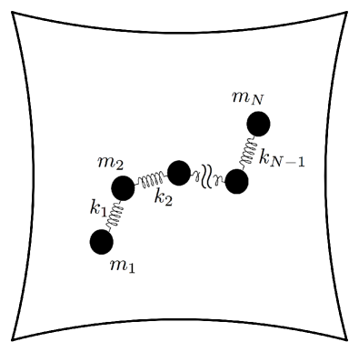
We now introduce the spring-chain system. It is composed of $N$ particles (masses) connected by $N-1$ massless springs. The masses can rotate smoothly on the $xy$-plane, as shown in Fig. 1. The system is defined by the following Lagrangian $L$:

$$L = \sum_{i=1}^{N}\frac{m_{i}}{2}\left(\dot{x}_{i}^{2}+\dot{y}_{i}^{2}\right)-\sum_{i=1}^{N-1}\frac{k_{i}}{2}\left\{\left|\overrightarrow{r_{i+1}}-\overrightarrow{r_{i}}\right|-\ell_{i}\right\}^{2}$$ (1)

$$- U(\left\{\overrightarrow{r_{i}}\right\})\ ,$$

where $m_{i}$ is the mass of the $i$’th particle, $\overrightarrow{r_{i}}\equiv(x_{i},y_{i})$ represents the position of the $i$’th particle, $k_{i}$ and $\ell_{i}$ are the spring constant and natural length of the $i$’th spring, respectively. $U$ is an external potential. In this paper we consider the case of $m_{i}=m$, $k_{i}=k$, and $\ell_{i}=\ell$ for all $i$. We set $m=1$ and $\ell=1$. The spring-chain model is a kind of beads-type models, which are used as models of polymer and protein Rouse (1953); Doi (1996); Wales (2003); Wolynes et al. (1995); Honeycutt and Thirumalai (1990).

Figure 1: A schematic illustration of spring-chain model.

III Method of Numerical Integration

We integrate the equation of motion of the model by a fourth-order symplectic integrator that is the composition of three successive second-order symplectic integrators. External potential Konishi and Yanagita (2009) $U(\overrightarrow{r})=0.01\sum_{j=1}^{N_{wall}}\left|\left|\overrightarrow{r}-\overrightarrow{R}_{j}\right|-a\right|^{-6}$ is applied in order to break the rotational symmetry and thus prevent the conservation of angular momentum. Here $N_{wall}=4$, $a=4N\ell$, $\vec{R_{j}}\equiv(R,0)$, $(0,R)$, $(-R,0)$, $(0,-R)$, $R\equiv N\ell+\sqrt{a^{2}-N^{2}\ell^{2}}$.

Throughout this paper, the following parameters and initial condition are set $m_{i}=m=1$, $\ell_{i}=\ell=1$ for all $i$ and $x_{i}=i-(N+1)/2$, $y_{i}=0$ for all $i$, respectively. The values of system size and initial momentum for each simulation set will be defined in the subsequent sections.

IV Result

Next, we briefly summarize the relation between our numerical simulation and thermal equilibrium. Under most of the initial conditions considered for the present simulations, the system undergoes chaotic motion. Since the model has no conserved quantities other than the total energy, one may think that the states of the system attained in the course of a long-duration are well approximated by a microcanonical distribution. In that case, the distribution of the state of each particle in the chain can be approximated by a canonical distribution at a certain temperature, by considering the other particles in the chain as a heat bath. That is, the long-term average of kinetic energy of each particle, $\overline{K_{i}}(t)$, is equal to thermal average $\langle K_{i}\rangle$. Then, according to the principle of equipartition of energy, the average kinetic energy of each particle is the same:

$$\overline{K_{i}}(t) \equiv\frac{1}{t}\int_{0}^{t}\frac{m_{i}}{2}\left(\dot{x}_{i}(t^{\prime})^{2}+\dot{y}_{i}(t^{\prime})^{2}\right)dt^{\prime}$$

$$\underset{t\rightarrow\infty}{\longrightarrow}\langle K_{i}\rangle\equiv\frac{1}{Z}\int K_{i}\exp\left(-\beta H\right)dpdq$$

$$=k_{B}T\,,$$ (2)

where $Z\equiv\int\exp\left(-\beta H\right)dpdq$, $\beta\equiv 1/k_{B}T$, $k_{B}$ is the Boltzmann constant, and $T$ is the temperature. Since our aim is to investigate the property of relaxation to equipartition, we define the following quantity in order to measure how close the system is to equipartition:

$$\Delta(t)\equiv\frac{1}{N}\sum_{i=1}^{N}\left[\overline{K_{i}}(t)-\left(\frac{1}{N}\sum_{i^{\prime}=1}^{N}\overline{K_{i^{\prime}}(t)}\right)\right]^{2}\,.$$ (3)

If $\Delta(t)=0$, then $\overline{K_{i}}(t)=K_{0}$ for all $i$. Similar quantities have been used to measure the degree of equipartition in studies on a supercooled liquid Thirumalai et al. (1989), self-gravitating systems Tsuchiya et al. (1994, 1996, 1997), and proteins Sagnella et al. (2000).

Figure 2: $\overline{K_{i}}(t)$ vs. $t$ for $k=10^{4}$. $N=8$. Plots are measured at 10 successive times: $t=10^{5}$ (blue circles), $2\times 10^{5}$ (red squares), $4\times 10^{5}$ (yellow diamonds), $8\times 10^{5}$ (green triangles), and $1.6\times 10^{6}$ (blue inverted triangles). The time step of integration $\delta t=4\times 10^{-4}$. The initial conditions are $x_{i}=i-(N+1)/2$, $y_{i}=0$, $p^{x}_{i}=0$, and $p^{y}_{1}=0.1$, $p^{y}_{i}=-0.1$ $(i\geq 2)$.

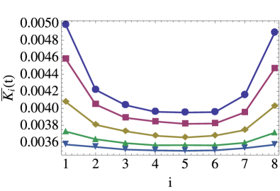
Figure 2 shows the time evolution of the profile of $\left\{\overline{K_{i}}(t),\ i=1,2,\cdots,N=8\right\}$. It is clearly observed that in the initial stage of the time evolution, the average kinetic energy of all particles is not equal; rather, particles near both the ends of the chain have a larger average $K_{i}$. The profile is similar to that of the rigid link, i.e., the planar chain model Konishi and Yanagita (2009). Then, as time progresses, differences in average $K_{i}$ among particles gradually decrease and tend to zero, and equipartition is achieved.

Figure 3: Time evolution of $\Delta(t)$ for $k=1$ (blue circles), $10$ (red squares), $10^{4}$ (yellow diamonds), and $10^{5}$ (green triangles). The other parameters and initial conditions are the same as those mentioned in the caption of Fig. 2. The dashed line represents $0.001/t$.

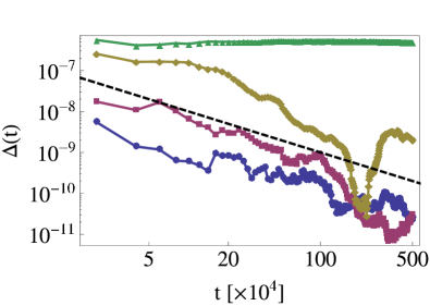
Figure 3 shows the relaxation of $\Delta(t)$ [Eq. (3)] for the data considered in Fig. 2. We observe that the system relaxes to equilibrium with the progress of time.

The physical process of relaxation can be understood by examining the kinetic energy in greater detail. We rewrite the Hamiltonian as

$$H = K_{vib}\bigl{(}\overrightarrow{\dot{\ell}}\bigr{)}+K_{rot}\bigl{(}\overrightarrow{\dot{\varphi}}\bigr{)}+K_{int}\bigl{(}\overrightarrow{\dot{\ell}},\overrightarrow{\dot{\varphi}}\bigr{)}+U(\overrightarrow{r})$$ (4)

$$K_{vib} \equiv \frac{M}{2}\sum_{j,k=1}^{N-1}\mu_{\min(j,k)}^{\leq}\mu_{\max(j,k)}^{>}\dot{\ell}_{j}\dot{\ell}_{k}\cos(\varphi_{j}-\varphi_{k})\,,$$

$$K_{rot} \equiv \frac{M}{2}\sum_{j,k=1}^{N-1}\mu_{\min(j,k)}^{\leq}\mu_{\max(j,k)}^{>}\ell_{j}\ell_{k}\dot{\varphi}_{j}\dot{\varphi}_{k}\cos(\varphi_{j}-\varphi_{k})\,,$$

$$K_{int} \equiv M\sum_{j,k=1}^{N-1}\mu_{\min(j,k)}^{\leq}\mu_{\max(j,k)}^{>}\dot{\ell}_{j}\ell_{k}\dot{\varphi}_{k}\sin(\varphi_{j}-\varphi_{k})\,,$$

where

$$M\equiv\sum_{i=1}^{N}m_{i},\ \mu_{k}\equiv\frac{m_{k}}{M},\ \ \mu_{n}^{\leq}\equiv\sum_{k=1}^{n}\mu_{k}\ ,\ \ \mu_{n}^{>}\equiv\sum_{k=n+1}^{N}\mu_{k}\,.$$ (5)

Figure 4: Time evolution of $\Delta^{(1)}(t;\tau)$ (blue circles) and $K_{vib}/K_{rot}$ (red squares). $N=8$, $K=100$, and $\delta t=10^{-3}$. $\tau=2\times 10^{3}.$ The initial conditions are $x_{i}=i-(N+1)/2$, $y_{i}=0$, $p^{x}_{i}=0$, $p^{y}_{i}=0.1$ ($i=1$), and $p^{y}_{i}=-0.1$ $(2\leq i\leq 8)$ .

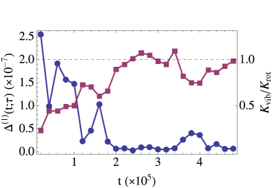
If equipartition is achieved, $\langle K_{vib}\rangle=\langle K_{rot}\rangle$, because the model has the same number of springs and angles. Figure 4 shows the temporal evolution of $\Delta^{(1)}(t;\tau)$ and $\overline{K_{vib}}(t;\tau)/\overline{K_{rot}}(t;\tau)$ for $k=200$. Here, the time average with two arguments, $\overline{f}(t;\tau)$, is defined as

$$\overline{f}(t;\tau)\equiv\frac{1}{\tau}\int_{t}^{t+\tau}f(t^{\prime})dt^{\prime}\,,$$ (6)

and

$$\Delta^{(1)}(t;\tau)\equiv\frac{1}{N}\sum_{i=1}^{N}\left[\overline{K_{i}}(t;\tau)-\left(\frac{1}{N}\sum_{i^{\prime}=1}^{N}\overline{K_{i^{\prime}}(t;\tau)}\right)\right]^{2}\,.$$ (7)

We find that the system relaxed to equipartition on a timescale similar to that on which the rotational energy $K_{rot}$ transformed into vibrational energy $K_{vib}$.

As mentioned earlier, the aim of this study is to examine the property of relaxation to equipartition of energy for the model expressed in Eq. (1). First, for each sample orbit starting from different initial condition, we define the relaxation time $t_{relax}^{(sample)}$ as the time required for $\Delta(t)$ to decay below a critical value $\Delta_{0}$. We define the average relaxation time over $N_{sample}$ orbits as

$$t_{relax}\equiv\frac{1}{N_{sample}}\sum_{sample}t_{relax}^{(sample)}.$$ (8)

This time is a measure of the relaxation time to equipartition.

Figure 5: $k$ dependence of average relaxation time $t_{relax}$. At each $k$ value, 15 samples are taken. Threshold value $\Delta_{0}=10^{-7}$. The time step $\delta t$ of integration is scaled as $\delta t=0.125*\sqrt{10}/\sqrt{k}$. The error bars represent standard deviations of $t_{relax}^{(sample)}$ for 15 samples. The dashed line shows $t_{relax}=5.52\times 10^{4}\exp(0.415\sqrt{k})$ obtained by fitting.

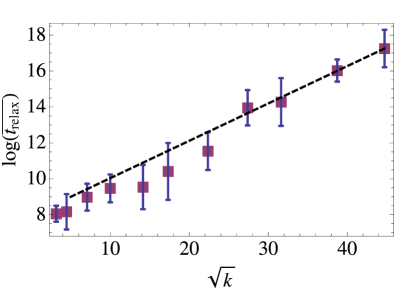
Figure 5 shows the plot of the dependence of $t_{relax}$ on the spring constant $k$. We observe that as the stiffness of the spring increases, the relaxation time increases rapidly. That is, systems with hard springs or a steep potential show rigid-like behavior of energetic particles near the chainends for a very long time, as shown in Fig. 2, before relaxing to equipartition.

Here, we mention a technical detail about the numerical integration used for obtaining the plot in Fig. 5. With increasing spring constant $k$, the period of bond-stretching vibration decreases in proportion to $1/\sqrt{k}$. Therefore, for large values of $k$, the magnitude of the time step of numerical integration should be reduced. We confirmed that $t_{relax}$ converges at $\delta t=0.125$ for $k=10$. Thus, we used $\delta t=0.125*\sqrt{10}/\sqrt{k}$ for each $k$.

On changing the initial conditions, the relaxation time $t_{relax}^{(sample)}$ changes, and we obtain a distribution of $t_{relax}^{(sample)}$, denoted as $P(t_{relax})$.

Figure 6: Distribution of $t_{relax}$ for $k=100$ (blue circles) and $k=200$ (red squares). For each value of $k$, the numbers of samples are 200. Both distributions are shown on a semi-log scale. The dashed lines show $P(t_{relax})=c\exp(-\alpha t_{relax})$. For $k=100$, $c=0.544$ and $\alpha=5.39\times 10^{-6}$. For $k=200$, $c=0.271$ and $\alpha=1.54\times 10^{-6}$.

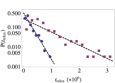
Figure 6 shows the distribution of $t_{relax}$ for $k=20$ and $k=100$. For both cases, the histograms show exponential decay expressed as

$$P(t_{relax})\propto\exp(-\alpha t_{relax})\,,$$ (9)

which suggests the existence of a characteristic timescale for the relaxation.

Next, we analyze the results of the abovementioned calculation using the concept of the Boltzmann-Jeans theory (also known as Boltzmann-Jeans conjecture) Benettin et al. (1989); Benettin (1994); Benettin and Fassò (1996); Benettin et al. (1987); Baldan and Benettin (1991); Benettin et al. (1993). The essence of this theory is roughly described as follows. ( For a detailed description of the theory please refer to Benettin et al. (1989). ) Suppose we have a system described by a Hamiltonian, which has two subsystems $H_{f}$ and $H_{s}$, their typical time scale being $\tau_{f}$ and $\tau_{s}$, respectively. Here, subscripts $f$ and $s$ denote “fast” and “slow,” respectively. Let us call $H_{f}$ and $H_{s}$ as a “fast subsystem” and “slow subsystem,” respectively. If the timescales of the fast and slow subsystems differ greatly, i.e., $\tau_{s}/\tau_{f}\gg 1$, then the timescale for the occurrence of energy exchange between these two subsystems is on the order of

$$t_{exch}\gtrsim\exp(c\frac{\tau_{s}}{\tau_{f}})\,.$$ (10)

That is, energy exchange occurs after a long time. In the case of the spring-chain system  [Eq. (1)] with a large spring constant $k$, the fast and slow subsystems correspond to bond vibration and relative rotation, respectively. Since the typical timescale of bond vibration is on the order of $2\pi\sqrt{m/k}$ and that of rotation is assumed to be constant, we have

$$t_{exch}\sim\exp(c\cdot 1/\sqrt{\frac{m}{k}})=\exp(c^{\prime}\sqrt{k})\,.$$ (11)

Since the relaxation to equipartition occurs by energy transfer from rotation to vibration (as we observed before), we can consider that $t_{exch}$ mentioned above is essentially the same as the relaxation time $t_{relax}$:

$$t_{relax}\sim\exp(c^{\prime}\sqrt{k})\,.$$ (12)

Now, we examine whether $t_{relax}$ obtained by the simulation obeys Eq. (12). The result is already shown in Fig. 5. $\mbox{Log}(t_{relax})$ is proportional to $\sqrt{k}$; therefore the interpretation by the Boltzmann-Jeans theory is appropriate.

This theory can also be used for interpreting the histogram of $t_{relax}^{(sample)}$. Since $t_{relax}$ is defined from the average of a number of samples, we have

$$t_{relax}=\int_{0}^{\infty}t_{relax}^{\prime}P(t_{relax}^{\prime})dt_{relax}^{\prime}\,,$$ (13)

where $P(t)$ is the distribution of $t_{relax}^{(sample)}$. If we adopt the exponential form for the distribution $P$ [Eq. (9)], then

$$t_{relax}=\frac{1}{\alpha}\,,$$ (14)

where $\alpha$ is the coefficient that appears in Eq. (9).

Combining Eqs. (12) and (14), the relation between the coefficient $\alpha$ and the spring constant should be

$$\alpha\propto\exp(-c^{\prime}\sqrt{k})\,.$$ (15)

A comparison between the estimation [Eq. (15)] and data is shown in Figure 7, from which we find that they are in good agreement.

Figure 7: Plot of $\alpha$ vs $k$, obtained from 300 samples. The dashed line shows $\log\alpha=c_{1}-c_{2}\sqrt{k}$, where $c_{1}=-3.93$ and $c_{2}=0.124$.

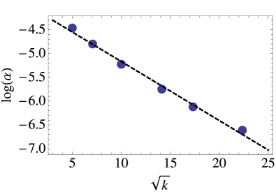
Thus, the fact that relaxation to equilibrium takes quite a long time to occur can be interpreted as the outcome of the Boltzmann-Jeans theory.

V Summary and Discussion

In this paper, we have numerically shown the occurrence of energetic motion of end particles for a 1D chain of point masses connected by hard springs. The timescale at which the energetic motion is observed depends on the spring constant, and this timescale lengthens with increasing the spring constant. Relaxation to equilibrium occurs as rotational kinetic energy is converted into vibrational kinetic energy.

The timescale of relaxation is estimated using the Boltzmann-Jeans theory, which describes the energy exchange rate in a system in which fast and slow motions coexist. In the case of our model, fast motion corresponds to bond vibration by a hard spring and slow motion corresponds to rotation and deformation of the chain. The result of our numerics is that the timescale is estimated as an exponential of the square root of the spring constant, which coincides well with simulation data.

The energetic motion of end particles is also observed in other systems, e.g., a planar chain system Konishi and Yanagita (2009) and multiple pendulum Oyama and Yanagita (1998); Saitoh et al. (1999); Saitoh and Yanagita (2000). These systems consist of masses connected by rigid links, and therefore, they are constrained systems. If we consider a rigid link as a limiting case of a hard spring when the spring constant $k$ is large ($k\rightarrow\infty$), then the spring-chain system examined in this study becomes a planar chain system when $k\rightarrow\infty$. Therefore, it is natural that the spatial energy distribution of the spring-chain system considered in this study resembles those of systems with rigid links.

However, the equilibrium behaviors of spring-chain system and rigid-link chain system are quite different. In the spring-chain system, equipartition achieved is of the usual form; that is, the average kinetic energy of each particle is the same, regardless of the magnitude of $k$. Then, chain-end particles in thermal equilibrium should not exhibit the energetic behavior. In contrast, in the rigid-link-chain system, chain-end particles behave energetically even in thermal equilibrium Konishi and Yanagita (2009). The energetic behavior of end particles in the spring-chain system is a transient behavior before the system relaxes to thermal equilibrium. What is important here is that the relaxation time increases with increasing the spring constant $k$ and that the relaxation time eventually diverges at $k\rightarrow\infty$. Therefore, a large $k$ value provides a good opportunity to observe energetic behavior in spring-chain systems.

The relaxation time to equipartition changes if we change the initial conditions. We found that the the relaxation time is distributed according to the exponential form for large relaxation time. This implies that relaxation occurs almost randomly. That is, the system moves on the energy surface in a random way and happens to encounter at which the system can divert toward the equipartition state. This situation is in contrast to the process of slow dynamics often observed in many Hamiltonian systems, where the relaxation time is often distributed according to the power law.

Slow relaxation is often observed in Hamiltonian systems, and in most cases, it is accompanied by strong temporal correlation caused by sticky or stagnant motion around KAM tori (regular orbits) and their remnants and $1/f$-type fluctuations. Such slow relaxation is observed in area-preserving mappings and some other high-dimensional systems Karney (1983); Chirikov and Shepelyansky (1984); Kohyama (1984); Geisel et al. (1987); Meiss and Ott (1986); Meiss (1986); Aizawa et al. (1989); Aizawa (1984); Yamaguchi and Konishi (1998). Such slow relaxation is explained by a hierarchical structure generally found in nearly integrable Hamiltonian systems. In this sense, it is quite common to find slow relaxation in Hamiltonian systems, if the Hamiltonian is nearly integrable.

However, the spring-chain model considered in this study is not nearly integrable. In addition, the systems which show slow relaxation in real world are not always nearly integrable. In contrast, the Boltzmann-Jeans theory is still applicable to Hamiltonian systems that are not nearly integrable and is able to explain the slow relaxation. Similar to the research by Shudo et al. Shudo et al. (2006), the result of our study also implies that the Boltzmann-Jeans theory can describe slow relaxation in more general systems other than the nearly integrable ones.

We used the Boltzmann-Jeans theory Benettin et al. (1989); Benettin (1994); Benettin and Fassò (1996); Benettin et al. (1987); Baldan and Benettin (1991); Benettin et al. (1993) to estimate the relaxation time. Although the concept of the theory dates back to the 19th century Boltzmann (1895); Jeans (1903, 1905), its importance is not very familiar and not many examples of the application of this theory have been demonstrated Shudo et al. (2006); Nakagawa and Kaneko (2000a, b); Nakagawa and Kaneko (2001); Morita and Kaneko (2004, 2005). Because the results of this study show that there is good agreement between numerical data and theoretical estimation, this study can be a good example of the applicability of the Boltzmann-Jeans theory.

In this study, we showed that chain-end particles behave energetically even for systems with a finite but large spring constant. This implies that similar behavior can be observed for natural chain-type systems that are not made of rigid links but whose intrachain potential between elements is very steep. The results of this study are expected to have many useful applications to polymers, proteins and some artificial objects.