Reptation quantum Monte Carlo for lattice Hamiltonians
with a directed-update scheme

Abstract

We provide an extension to lattice systems of the reptation quantum Monte Carlo (RQMC) algorithm, originally devised for continuous Hamiltonians. For systems affected by the sign problem, a method to systematically improve upon the so-called fixed-node approximation is also proposed. The generality of the method, which also takes advantage of a canonical worm algorithm scheme to measure off-diagonal observables, makes it applicable to a vast variety of quantum systems and eases the study of their ground-state and excited-states properties. As a case study, we investigate the quantum dynamics of the one-dimensional Heisenberg model and we provide accurate estimates of the ground-state energy of the two-dimensional fermionic Hubbard model.

I Introduction

The path-integral formulation of quantum mechanics is the foundation of many numerical methods that allow one to study with great accuracy the rich physics of interacting quantum systems. At finite temperature, a path-integral Monte Carlo (PIMC) technique for continuous systems has been developed and applied by Ceperley and Pollock.CepPoll ; Ceperley:1995 Recently, this approach has been renovated in a new class of methods known as worm algorithms. (Prokofev:1998, ; Boninsegni:2006, ) The zero-temperature counterparts of the PIMC algorithm are the reptation quantum Monte Carlo (RQMC) (Baroni:1999, ) and the path-integral ground state (PIGS) methods, (Sarsa:2000, ) which have been demonstrated useful to simulate coupled electron-ion systems, (Pierleoni, ) as well as to infer spectral properties from imaginary time dynamics. (Carleo:2009, ) A number of important physical problems –particularly in the fields of strongly correlated fermions and cold atoms– can be fruitfully modeled by lattice Hamiltonians. A first application of path-integral techniques to (boson) lattice models was proposed by Krauth et al. in 1991. (Krauth:1991, ) Few other attempts to apply PIMC to lattice models have been made ever since, with a recent application of the RQMC idea to the quantum dimer model Hamiltonian. (Syljuasen:2006, ) In this paper, we propose a new method that generalizes and improves the approach of Ref. Syljuasen:2006, in several ways. Our method is based on continuous-time random walks and is therefore unaffected by time-step errors. Inspired by the work of Syljuasen and Sandvik Sandvik:2002 and Rousseau, Rousseau:2008 we adopt a generalization of the bounce algorithm of Pierleoni and Ceperley, (Pierleoni, ) called directed updates, which helps reducing the correlation time in path sampling. We also introduce a worm-algorithm based method to calculate pure expectation values of arbitrary off-diagonal observables, which are generally out of the scope of existing lattice ground-state methods.

The resulting algorithm naturally applies to fermions, using the fixed-node approximation. A technique to improve systematically upon this approximation is proposed, based on the calculation of a few moments of the Hamiltonian. Our methodology is demonstrated by a few case studies on the one-dimensional Heisenberg and the two-dimensional fermion Hubbard models.

This paper is organized as follow: in Sec. II we present the general formalism of ground-state PIMC for lattice models; in Sec. III our implementation of the RQMC algorithm on a lattice is presented. In particular, we give a detailed account of the above mentioned directed update technique (Sec. III.1) and of the continuous-time propagator (Sec. III.2); in Sec. III.3, we introduce an extension of the algorithm to cope with off-diagonal observables, while in Sec. III.4 a further extension to systems affected by sign problems is presented, including a strategy to improve systematically upon the fixed-node approximation. Sec. IV contains a few case applications, including the simulation of the spectral properties and spin correlations of the one-dimensional Heisenberg model and the calculation of the ground-state energies of the fermionic Hubbard model with a significantly better accuracy than that achieved by the fixed-node approximation. In Sec. V we finally draw our conclusions.

II General formalism

Let us consider a generic lattice Hamiltonian $\hat{H}$ and a complete and orthogonal basis set, whose states are denoted by $|x\rangle$. Given the generic wave function $|\Psi\rangle$, its amplitude on the configuration $|x\rangle$ will be denoted by $\Psi(x)$, namely $\Psi(x)=\langle x|\Psi\rangle$. The exact ground-state wave function $|\Psi_{0}\rangle$ can be obtained by the imaginary time evolution of a given variational state $|\Psi_{V}\rangle$:

$$|\Psi_{0}\rangle\propto\lim_{\beta\rightarrow\infty}|\Psi_{\beta}\rangle,$$ (1)

where $|\Psi_{\beta}\rangle\equiv e^{-\beta\hat{H}}|\Psi_{V}\rangle$, provided that the variational state is non-orthogonal to $|\Psi_{0}\rangle$, i.e., $\langle\Psi_{V}|\Psi_{0}\rangle\neq 0$. Then, the ground-state expectation value of a quantum operator $\hat{O}$ can be obtained by

$$\langle\hat{O}\rangle=\lim_{\beta\rightarrow\infty}\frac{\langle\Psi_{\beta}|\hat{O}|\Psi_{\beta}\rangle}{\langle\Psi_{\beta}|\Psi_{\beta}\rangle}.$$ (2)

A practical computational scheme can be conveniently introduced by considering a path-integral representation of the imaginary time evolution. To such a purpose, we split the total imaginary time $\beta$ into $M$ slices of “duration” $\tau=\beta/M$, in such a way that the value of the evolved wave function on a generic many-body state of the system reads

$$\Psi_{\beta}(x_{0})=\sum_{x_{1}\dots x_{M}}\prod_{i=1}^{M}G_{x_{i-1}x_{i}}^{\tau}\Psi_{V}(x_{M}),$$ (3)

where we have introduced the imaginary time propagators

$$G_{x_{i-1}x_{i}}^{\tau}=\langle x_{i-1}|e^{-\tau\hat{H}}|x_{i}\rangle.$$ (4)

Within this approach, it is easy to write expectation values of operators $\hat{O}$ that are diagonal in the chosen basis $|x\rangle$, i.e., $\langle x|\hat{O}|y\rangle=O(x)\delta_{x,y}$. In fact, in this case we have that:

$$\langle\hat{O}\rangle=\lim_{\beta\rightarrow\infty}\frac{\sum_{\mathbf{X}}\Pi^{\beta}(\mathbf{X})O(x_{M})}{\sum_{\mathbf{X}}\Pi^{\beta}(\mathbf{X})},$$ (5)

where the summation is extended to all possible imaginary time paths $\mathbf{X}\equiv\{x_{0},x_{1},\dots,x_{2M}\}$, and $\Pi^{\beta}(\mathbf{X})$ is given by:

$$\Pi^{\beta}(\mathbf{X})=\Psi_{V}(x_{0})\left[\prod_{i=1}^{2M}G_{x_{i-1}x_{i}}^{\tau}\right]\Psi_{V}(x_{2M}).$$ (6)

The ground-state energy can be conveniently obtained by means of the mixed average:

$$E_{0}=\lim_{\beta\rightarrow\infty}\frac{\sum_{\mathbf{X}}\Pi^{\beta}(\mathbf{X})E_{L}(x_{0})}{\sum_{\mathbf{X}}\Pi^{\beta}(\mathbf{X})},$$ (7)

where $E_{L}(x)=\langle x|\hat{H}|\Psi_{V}\rangle/\langle x|\Psi_{V}\rangle$ is the so-called local energy.

Besides the static (i.e., equal-time) correlation functions, this formalism allows one to calculate also dynamical correlations in imaginary time $C_{AB}(\mathcal{T})=\langle\hat{A}(\mathcal{T})\hat{B}(0)\rangle$ that can be computed as

$$C_{AB}(\mathcal{T})=\lim_{\beta\rightarrow\infty}\frac{\sum_{\mathbf{X}}\Pi^{\beta}(\mathbf{X})A(x_{n})B(x_{m})}{\sum_{\mathbf{X}}\Pi^{\beta}(\mathbf{X})},$$ (8)

where $x_{n}$ and $x_{m}$ are two coordinates of the path such that $(m-n)\tau=\mathcal{T}$.

III Reptation quantum Monte Carlo

A probabilistic interpretation of the previous expectation values (5), (7), and (8) can be immediately recovered whenever $\Pi^{\beta}(\mathbf{X})\geq 0$ for all configurations $\mathbf{X}$. Indeed, in this case, $\Pi^{\beta}(\mathbf{X})$ can be interpreted as a probability distribution that may be readily sampled by using Monte Carlo algorithms. This fact allows ground-state expectation values to be calculated exactly, within statistical errors.

The basic idea of the RQMC algorithm is to sample the distribution probability $\Pi^{\beta}(\mathbf{X})$ by using a Markov process with simple moves. Given the configuration $\mathbf{X}\equiv\{x_{0},x_{1},\dots,x_{2M}\}$, a new configuration is proposed in two possible ways: either $\mathbf{X}_{L}\equiv\{x_{T},x_{0},\dots,x_{2M-1}\}$ (which we call “left move”) or $\mathbf{X}_{R}\equiv\{x_{1},\dots,x_{2M},x_{T}\}$, (which we call “right move”). In both cases, $x_{T}$ is a new configuration proposed according to a suitable transition probability $R^{\tau}(x\rightarrow x_{T})$, where $x$ stays for $x_{0}$ ($x_{2M}$) when the left (right) move is considered. Such “sliding moves” are depicted in Fig. 1. Ideally, the transition probability should guarantee the minimum possible statistical error on the desired observables and, to such a purpose, it has been proved useful to consider the propagator with importance sampling, i.e., $\tilde{G}_{xy}^{\tau}=G_{xy}^{\tau}\Psi_{V}(y)/\Psi_{V}(x)$ and take the following transition probability

$$R^{\tau}(x\rightarrow y)=\frac{\tilde{G}_{xy}^{\tau}}{w(x)},$$ (9)

where

$$w(x)=\sum_{x^{\prime}}\tilde{G}_{xx^{\prime}}^{\tau}$$ (10)

represents the normalization factor. The explicit form of $R^{\tau}(x\rightarrow x_{T})$ will be discussed in more detail in Sec. III.2. The proposed configuration $\mathbf{X}_{d}$ (where $d=L$ or $R$) is accepted or rejected according to the usual Metropolis algorithm, where the acceptance rate is given by:

$$A=\min\left\{1\,,\,\frac{\Pi^{\beta}(\mathbf{X}_{d})R^{\tau}(x_{T}\rightarrow x)}{\Pi^{\beta}(\mathbf{X})R^{\tau}(x\rightarrow x_{T})}\right\}.$$ (11)

In this way, a sequence of configurations $\mathbf{X}^{k}$ is generated, $k$ being the (discrete) time index of the Markov chain.

Figure 1: Pictorial representation of the “sliding moves” along the right imaginary time direction. In the new configuration (bottom), a new head for the reptile is generated from the old configuration (top) and the tail is discarded.

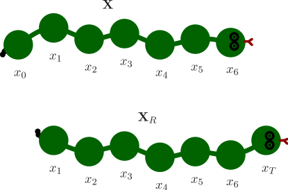
In order to reduce the auto-correlation time of the observables it is convenient to make several consecutive sliding moves along the same imaginary time direction. Baroni:1999 To such a purpose, a recent development called “bounce” algorithm has been proposed. Pierleoni Although the bounce algorithm sampling procedure does not fulfill the microscopic detailed balance, the equilibrium probability $\Pi^{\beta}(\mathbf{X})$ is correctly sampled. Pierleoni The RQMC algorithm with bounce moves can be then summarized in the following steps:

1. For the current direction of the move and for the present configuration $\mathbf{X}^{k}$, propose $x_{T}$ according to the transition probability $R^{\tau}(x\rightarrow x_{T})$, where $x=x_{0}^{k}$ if $d=L$ and $x=x_{2M}^{k}$ if $d=R$.

2. Given the form of the acceptance ratio $A$ of Eq. (11), accept the proposed configuration according to the probability

   $$A_{L}=\min\left\{1\,,\,\frac{w(x_{0}^{k})}{w(x_{2M-1}^{k})}\right\},$$ (12)

   if $d=L$, or with probability

   $$A_{R}=\min\left\{1\,,\,\frac{w(x_{2M}^{k})}{w(x_{1}^{k})}\right\},$$ (13)

   if $d=R$.

3. If the move is accepted, update the path configurations according to $\mathbf{X}^{k+1}=\mathbf{X}_{d}$ and continue along the same direction, otherwise $\mathbf{X}^{k+1}=\mathbf{X}^{k}$ and change direction.

4. Go back to 1.

III.1 Directed updates

At this point we introduce a novel alternative sampling approach, which generalizes the bounce idea while strictly fulfilling the detailed balance condition. Such a scheme, which is largely inspired by the loop algorithm methods devised for the stochastic series expansion (Sandvik:2002, ; Sandvik:1999, ) and for the worm algorithm, (Rousseau:2008, ; Rombouts:2006, ) allows one to choose the time direction in a purely Markovian way, i.e., independently of the previous history.

In our algorithm, a Markov step consists of many simple consecutive “sliding moves”, whose number is not fixed a-priori but is determined by a certain probability (see below). The actual Monte Carlo step takes place at the end of few consecutive updates along the currently chosen direction. In the examples below, we denote the number of these sliding moves between two Monte Carlo steps by $s$.

At the beginning of each Markov step we choose a direction $d$ according to the probability $P(\mathbf{X}^{k},d)$, whose form will be specified later. Assuming that the right direction has been chosen, we propose a new configuration $x_{T}$, according to the transition probability $R^{\tau}(x_{2M}^{k}\rightarrow x_{T})$ and the configuration labels are shifted according to $\mathbf{X}^{k+1}=\{x_{1}^{k},\dots,x_{2M}^{k},x_{T}\}$, with $x_{2M}^{k+1}=x_{T}$. At this point, we continue updates along this direction with probability $K(\mathbf{X}^{k+1},\rightarrow)$, or stop with probability $[1-K(\mathbf{X}^{k+1},\rightarrow)]$. If it has been decided to continue the updates, then a new configuration is generated according to $R^{\tau}(x_{2M}^{k+1}\rightarrow x_{T})$ and the labels of the configuration are again shifted according to $\mathbf{X}^{k+2}=\{x_{1}^{k+1},\dots,x_{2M}^{k+1},x_{T}\}$. The Markov step finishes after $s$ consecutive updates along the right direction only when $K(\mathbf{X}^{k+s},\rightarrow)<\xi_{s}$, where $\xi_{s}$ is a random number uniformly distributed in $[0,1)$. At this point a Metropolis test should be done, in order to accept or reject the sequence of intermediate $s$ sliding moves:

$$A=\min\left\{1,\frac{q(\mathbf{X}^{k+s})}{q(\mathbf{X}^{k})}\right\},$$ (14)

where (see Appendix A)

$$q(\mathbf{X}) = \frac{P(\mathbf{X},\leftarrow)}{1-K(\mathbf{X},\rightarrow)}w(x_{2M-1})$$ (15)

$$= \frac{P(\mathbf{X},\rightarrow)}{1-K(\mathbf{X},\leftarrow)}w(x_{1}).$$

However, in order to avoid time-consuming restorations of the original configuration, it is preferable to accept all the moves, while keeping track of the residual weight $q(\mathbf{X})$. This is possible since $A$ only depends upon initial and final configurations, so that, given that all the intermediate moves are accepted, the sampled distribution probability is $\Pi^{\beta}(\mathbf{X})\times q(\mathbf{X})$. The contribution of the current configuration to statistical averages must be then weighted by the factor $1/q(\mathbf{X})$.

To proceed to the next Markov step, a new direction $d$ is chosen according to $P(\mathbf{X}^{k+s},\leftarrow)$ and $P(\mathbf{X}^{k+s},\rightarrow)$ and the updates are carried along the extracted new direction.

Let us now show the actual expressions for the afore-mentioned probabilities. In Appendix A, it is demonstrated that the detailed balance is satisfied if one chooses the probabilities for the directions as

$$P(\mathbf{X},\leftarrow) = \frac{1}{1+a(\mathbf{X})},$$ (16)

$$P(\mathbf{X},\rightarrow) = \frac{a(\mathbf{X})}{1+a(\mathbf{X})},$$ (17)

where

$$a(\mathbf{X})=\frac{w(x_{2M-1})}{w(x_{1})}\frac{1-K(\mathbf{X},\leftarrow)}{1-K(\mathbf{X},\rightarrow)},$$ (18)

which is positive and, therefore, guarantees that the above defined quantities are well defined probabilities, i.e., $0\leq P(\mathbf{X},\leftarrow)\leq 1$ and $0\leq P(\mathbf{X},\rightarrow)\leq 1$, with the additional property that $P(\mathbf{X},\leftarrow)+P(\mathbf{X},\rightarrow)=1$.

Regarding the probabilities to continue the updates along the current direction, we have a substantial freedom of choice, provided that the condition $\frac{K(\mathbf{X},\leftarrow)}{K(\mathbf{X},\rightarrow)}=\frac{w(x_{1})}{w(x_{2M-1})}$, is satisfied (see Appendix A). In this paper we have adopted

$$K(\mathbf{X},\leftarrow) = \alpha\min\left\{1,b(\mathbf{X})\right\},$$ (19)

$$K(\mathbf{X},\rightarrow) = \alpha\min\left\{1,\frac{1}{b(\mathbf{X})}\right\},$$ (20)

where we have defined:

$$b(\mathbf{X})=\frac{w(x_{1})}{w(x_{2M-1})}.$$ (21)

and $0<\alpha<1$ is an arbitrary parameter of the algorithm, which controls the average number of consecutive updates along the same direction.

Summarizing, the RQMC algorithm with directed updates consists of a sequence of Markov steps determined by the following rules:

1. Choose a time direction $d$ according to the probabilities of Eqs. (16) and (17).

2. Propose a new configuration $x_{T}$ according to the transition probability $R^{\tau}(x\rightarrow x_{T})$, where $x=x_{0}^{k}$ if $d=L$ and $x=x_{2M}^{k}$ if $d=R$.

3. Shift the configuration indexes according to $\mathbf{X}^{k+1}=\{x_{T},x_{0}^{k},\dots,x_{2M-1}^{k}\}$ if $d=L$ or $\mathbf{X}^{k+1}=\{x_{1}^{k},\dots,x_{2M}^{k},x_{T}\}$ if $d=R$.

4. According to the probability $K(\mathbf{X}^{k},\rightarrow)$ or $K(\mathbf{X}^{k},\leftarrow)$, decide whether keep moving in the same direction or change direction. In the former case, go to 2, otherwise go to 5.

5. The Markov step ends here and the current configuration carries the weight $1/q(\mathbf{X}^{k+s})$, where $s$ is the number of intermediate moves along the direction chosen.

The relationship between the directed update scheme and the bounce algorithm is further elucidated in Appendix B, where general considerations about the efficiency of the algorithms are presented.

III.2 Continuous-time propagator

One of the most striking differences between the original formulation of the RQMC on the continuum and the present formulation on the lattice is the lack of the discretization error appearing in the Trotter decomposition of the propagator. Indeed it is easier to carry the propagation in continuous imaginary time on a lattice, (Capriotti:2000, ) than on the continuum. (Lee:2005, ) To such a purpose, let us consider the limit of an infinitesimal imaginary time $\epsilon$, for which the transition probability of Eq. (9) can be written as

$$R^{\epsilon}(x\rightarrow y)\simeq\frac{\delta_{xy}-\epsilon\Psi_{V}(y)H_{xy}/\Psi_{V}(x)}{1-\epsilon E_{L}(x)}$$ (22)

$$\simeq\delta_{xy}\left[1+\epsilon E_{L}(x)\right]-\epsilon\left[H_{xy}\frac{\Psi_{V}(y)}{\Psi_{V}(x)}\right]+o(\epsilon^{2}),$$ (23)

where $E_{L}(x)$ is the previously defined local energy and $H_{x,y}=\langle x|H|y\rangle$ denotes the matrix element of the Hamiltonian. Whenever $\Psi_{V}(y)H_{xy}/\Psi_{V}(x)$ is non positive for all $x$ and $y$, this equation takes the form of a continuous-time Markov process, whose analytical properties are well known. In particular, the probability distribution for the “waiting time” $\tau_{w}$ in a given state $x$, i.e., the average time that the system spends in the state $x$ before making an off-diagonal transition to another state $y\neq x$, is exactly known, namely $P(\tau_{w};x)=\exp\{-\tau_{w}\left[H_{xx}-E_{L}(x)\right]\}$. As a consequence, the finite-time propagator $R^{\tau}(x\rightarrow y)$ can be directly sampled, giving rise to a succession of a certain number $n$ of consecutive transitions $x\rightarrow z_{1}\rightarrow z_{2}\rightarrow\dots\rightarrow y$, with corresponding waiting times $\tau_{w}(z_{i})$ (such that $\sum_{i}\tau_{w}(z_{i})=\tau$). The normalization of the whole process is

$$w(x)=\exp\left[-\sum_{i}\tau_{w}(z_{i})E_{L}(z_{i})\right],$$ (24)

where the waiting times are extracted according to the exponential probability $P(\tau_{w};z_{i})$. The transitions between the intermediate configurations are done according to the off-diagonal elements of Eq. (23), i.e., $z_{i+1}$ is chosen with probability proportional to $\left[-\Psi_{V}(z_{i+1})H_{z_{i}z_{i+1}}/\Psi_{V}(z_{i})\right]$.

III.3 Off-diagonal observables

The formalism so-far developed allows one to successfully compute pure ground-state expectation values of operators that are diagonal in the local basis $x$, with the expectation values of off-diagonal operators restricted to the so-called mixed averages. Baroni:1999 ; Sarsa:2000 ; Capriotti:2000 Nonetheless, it is often of great interest to remove such a limitation (whose result is biased by the quality of the variational wave function) and a dedicated sampling strategy has to be devised in order to cope with such a need. In the following, we show that a relatively easy modification of the sampling scheme can accomplish this task, providing us with a general tool to compute ground-state averages of operators that are non local in the chosen basis $x$.

Let us consider an arbitrary off-diagonal observable $\hat{\mathcal{O}}$, which can be in turn considered as the summation of many observables we are interested in, i.e., $\hat{\mathcal{O}}=\sum_{d}\hat{\mathcal{O}}^{(d)}$. For example, we can imagine these operators to be the components of the one-body density matrix at a given distance, $\hat{\mathcal{O}}^{(d)}=\sum_{\left\langle r,r^{\prime}\right\rangle_{d}}b_{r}^{\dagger}b_{r^{\prime}}$ with the summation extended to all lattice coordinates at a fixed distance $d$.

In the spirit of Refs Rombouts:2006, ; Rousseau:2008, we introduce a worm-operator defined by

$$\mathcal{W}_{x,y}=\delta_{x,y}+\lambda\mathcal{O}_{x,y},$$ (25)

where $\lambda$ is a positive constant, and consider the extended configuration space spanned by the paths

$$\Pi_{\mathcal{W}}^{\beta}(\mathbf{X}) = \Psi_{V}\left(x_{0}\right)\times\prod_{i=1}^{L}G_{x_{i-1}x_{i}}^{\tau}\times\mathcal{W}_{x_{L}x_{R}}\times$$ (26)

$$\times \prod_{i=R+1}^{2M+1}G_{x_{i-1}x_{i}}^{\tau}\times\Psi_{V}\left(x_{2M+1}\right).$$

The extended paths are broken in two (space)-discontinuous pieces by the worm operator, which is placed at an imaginary-time $0\leq\tau_{LR}\leq\beta$. Therefore, paths contain $2(M+1)$ coordinates, including $x_{L}$ and $x_{R}$ that refer to the same imaginary time $\tau_{LR}$.

The configuration space spanned by Eq. (26) is clearly larger than the one spanned by Eq. (6), which is recovered whenever $x_{L}=x_{R}$, i.e., when the worm operator is diagonal.

The pure ground-state expectation value of the operator $\hat{\mathcal{O}}$ is conveniently written in terms of the extended paths as

$$\langle\hat{\mathcal{O}}\rangle=\frac{1}{\lambda}\lim_{\beta\rightarrow\infty}\frac{\sum_{\mathbf{X}}\Pi_{\mathcal{W}}^{\beta}(\mathbf{X})\times\Theta(x_{L}\neq x_{R})}{\sum_{\mathbf{X}}\Pi_{\mathcal{W}}^{\beta}(\mathbf{X})\times\Theta(x_{L}=x_{R})},$$ (27)

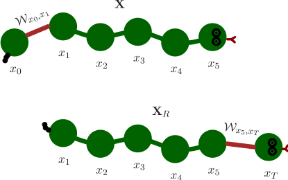
where $\Theta(C)\neq 0$ whenever condition $C$ is satisfied. The modulus of Eq. (26) can be in turn interpreted as a probability distribution and stochastically sampled by means of the elementary sliding moves considered before. Indeed, whenever the worm operator is far from the ends of the imaginary-time paths, the sampling scheme remains unchanged. In this case, a move along direction $d$ will generate a new head (or tail) for the reptile according to $R^{\tau}(x\rightarrow x_{T})$ while shifting the worm position of $\pm\tau$. On the other hand, whenever the worm operator reaches the ends of the reptile, a new worm configuration is proposed on the other side; in analogy with the previous analysis, new configurations are generated according to a transition probability

$$R^{\mathcal{W}}(x\rightarrow y)=\frac{1}{\bar{w}(x)}\left|\mathcal{W}_{xy}\frac{\psi_{V}(y)}{\psi_{V}(x)}\right|,$$ (28)

where $\bar{w}(x)$ is the normalization factor. Due to the particular form of the matrix elements (25), the transition probability will lead either to diagonal configurations $(x=y)$ or to off-diagonal configurations $(x\neq y)$, thus generating continuous and discontinuous paths. The relative probability for diagonal and off-diagonal configurations depends on the value of $\lambda$ that can be tuned in order to reach a balanced sampling frequency for the different sectors of the extended paths. In order to exemplify the worm updates, let us consider the case in which $d=R$ and a configuration $\Psi_{V}\left(x_{0}\right)\mathcal{W}_{x_{0}x_{1}}\left[\prod_{i=2}^{2M+1}G_{x_{i-1}x_{i}}^{\tau}\right]\Psi_{V}\left(x_{2M+1}\right)$, after a sliding update in the right direction, we will have $\Psi_{V}\left(x_{1}\right)\left[\prod_{i=2}^{2M+1}G_{x_{i-1}x_{i}}^{\tau}\right]\mathcal{W}_{x_{2M+1}x_{T}}\Psi_{V}\left(x_{T}\right)$, where $x_{T}$ is proposed according to the transition probability $R^{\mathcal{W}}(x_{2M+1}\rightarrow x_{T})$ (see Fig. 2). In analogy with the previous case, the acceptance factor for the bounce moves reads $\bar{A}_{R}=\min\left\{1\,,\,\frac{\bar{w}(x_{2M+1})}{\bar{w}(x_{1}^{k})}\right\}$.

Figure 2: Pictorial representation of the “sliding moves” along the right imaginary-time direction when the worm operator sits at the tail of the reptile. In the new configuration (bottom), a new head for the reptile is generated from the old configuration (top), the old tail configuration is discarded and the worm discontinuity is moved to the “neck” of the reptile.

Summarizing, the RQMC with worm-updates consists of the following steps:

1. For the current direction of the move $d$ and for the present configuration $\mathbf{X}^{k}$ consider the worm-operator position $\tau_{LR}$.

2. If the worm is not at the ends of the reptile (i.e., $\tau_{LR}\neq 0$ when $d=L$ and $\tau_{LR}\neq\beta$ when $d=R$) go to step (a), otherwise go to step (b).

   1. Propose a new configuration $x_{T}$ according to the transition probability $R^{\tau}(x\rightarrow x_{T})$, where $x=x_{0}^{k}$ if $d=L$ and $x=x_{2M+1}^{k}$ if $d=R$. The new configuration is accepted with probability

      $$A_{L}=\min\left\{1\,,\,\frac{w(x_{0}^{k})}{w(x_{2M}^{k})}\right\},$$ (29)

      if $d=L$, or with probability

      $$A_{R}=\min\left\{1\,,\,\frac{w(x_{2M+1}^{k})}{w(x_{1}^{k})}\right\},$$ (30)

      if $d=R$. In the proposed state $\mathbf{X}_{d}$, all the configuration labels are shifted in the $d$ direction, determining in turn a shift of the worm operator of a time interval $\pm\tau$, depending on $d$.

   2. Propose a new configuration $x_{T}$ according to the worm transition probability $R^{\mathcal{W}}(x\rightarrow x_{T})$, where $x=x_{L}^{k}=x_{0}^{k}$ if $d=L$ and $x=x_{R}^{k}=x_{2M+1}^{k}$ if $d=R$. Accept the new configuration with probability

      $$\bar{A}_{L}=\min\left\{1\,,\,\frac{\bar{w}(x_{0}^{k})}{\bar{w}(x_{2M}^{k})}\right\},$$ (31)

      if $d=L$, or with probability

      $$\bar{A}_{R}=\min\left\{1\,,\,\frac{\bar{w}(x_{2M+1}^{k})}{\bar{w}(x_{1}^{k})}\right\},$$ (32)

      if $d=R$. In the proposed state $\mathbf{X}_{d}$, all the configuration labels are shifted in the $d$ direction, and the worm operator is moved from the head (tail) to the tail (head) of the reptile, depending on $d$.

3. If the move is accepted, update the path configurations according to $\mathbf{X}^{k+1}=\mathbf{X}_{d}$ and continue along the same direction, otherwise $\mathbf{X}^{k+1}=\mathbf{X}^{k}$ and change direction.

4. Go back to 1.

This scheme samples the probability density associated to the modulus of Eq. (26), and the expectation values of the individual components $\mathcal{\hat{O}}_{d}$ can be recast as statistical averages over such a probability distribution, while keeping track of the overall sign of the extended paths. In particular the best estimate of the ground-state expectation values is obtained when the worm is in the central part of the path, at $\tau_{LR}=\beta/2$, leading to

$$\langle\hat{\mathcal{O}}^{(d)}\rangle=\frac{\sum_{\mathbf{X}}\Pi_{\mathcal{W}}^{\beta}(\mathbf{X})\times\Theta\left(\mathcal{O}_{x_{L}x_{R}}^{(d)}\neq 0,\,\tau_{LR}=\frac{\beta}{2}\right)}{\sum_{\mathbf{X}}\Pi_{\mathcal{W}}^{\beta}(\mathbf{X})\times\Theta\left(x_{L}=x_{R},\,\tau_{LR}=\frac{\beta}{2}\right)}$$

$$=\frac{1}{\lambda}\frac{\left\langle\Theta\left(\mathcal{O}_{x_{L}x_{R}}^{(d)}\neq 0\right)\times\text{sign}\left[\Pi_{\mathcal{W}}^{\beta}(\mathbf{X})\right]\right\rangle_{\text{OD}}^{\text{center}}}{N_{D}^{\text{center}}},$$ (33)

where $\left\langle\dots\right\rangle_{\text{OD}}^{\text{center}}$ denotes statistical averages over the off-diagonal distribution $\left|\Pi_{\mathcal{W}}^{\beta}(\mathbf{X})\right|\Theta(x_{L}\neq x_{R},\,\tau_{LR}=\frac{\beta}{2})$ and $N_{D}^{\text{center}}$ is the number of configurations sampled with a diagonal worm operator in the center of the paths.

III.4 Tackling the sign problem

When the probability distribution of Eq. (6) is not positive defined, as is generally the case with fermions, the probabilistic interpretation of the imaginary time paths breaks down. This circumstance, which is known as “sign problem”, originates whenever $\Psi_{V}(y)H_{xy}/\Psi_{V}(x)>0$ for some element $x\neq y$. In this case, it is not possible to have polynomial algorithms that are able to obtain an exact solution of the problem, which would imply to sample correctly the resulting signs. Therefore, approximated schemes are welcome and often adopted, the most widespread one being the so-called fixed-node (FN) approximation. For lattice systems, this approach relies on the definition of an effective Hamiltonian, which depends parametrically on the nodal structure of a given variational wave function $\Psi_{V}(x)=\langle x|\Psi_{V}\rangle$. CeperleyFN The matrix elements of the FN Hamiltonian are defined as

$$H_{xy}^{\text{{fn}}}=\begin{cases}H_{xx}+\nu_{\text{sf}}(x)&\text{if}\,\,x=y\\ H_{xy}&\text{if}\,\,\Psi_{V}(y)H_{xy}\Psi_{V}(x)\leq 0\\ 0&\text{if}\,\,\Psi_{V}(y)H_{xy}\Psi_{V}(x)>0\end{cases}$$ (34)

where the sign-flip potential is $\nu_{\text{sf}}(x)=\sum_{y:\text{sf}}\Psi_{V}(y)H_{xy}/\Psi_{V}(x)$, the sum being extended to all the sign-flip states defined by the condition $\Psi_{V}(y)H_{xy}\Psi_{V}(x)>0$. With such a choice, the transition matrix $R^{\epsilon}(x\rightarrow y)$ of Eq. (23) is always positive definite and the summation of Eq. (3) is now restricted –which results in the FN approximation– to a region of the Hilbert space in which imaginary time paths are positive definite. Therefore, within the FN approximation, the ground-state wave function $|\Psi^{\text{fn}}\rangle$ of $\hat{H}^{\text{fn}}$ can be stochastically sampled without any sign problem. Moreover, it is easy to show that the FN approximation becomes exact whenever the signs of the exact ground state are known. Most importantly, it has been proven CeperleyFN that the FN ground-state energy $E^{\text{fn}}=\langle\hat{H}^{\text{fn}}\rangle$ gives a rigorous upper-bound to the exact ground-state one and improves the pure variational results.

At this point, we introduce a straightforward, although computationally expensive, way to improve further the FN energy. Our strategy amounts to compute the expectation values of arbitrary powers of the original Hamiltonian $\hat{H}$ on the FN ground state $|\Psi_{\text{fn}}\rangle$, namely

$$L_{k}=\frac{\langle\Psi_{\text{fn}}|\hat{H}^{k}|\Psi_{\text{fn}}\rangle}{\langle\Psi_{\text{fn}}|\Psi_{\text{fn}}\rangle}.$$ (35)

The FN ground state can be expanded in the basis set of the eigenstates of $\hat{H}$ as $|\Psi_{\text{fn}}\rangle=\gamma_{0}|\Psi_{0}\rangle+\gamma_{1}|\Psi_{1}\rangle+\gamma_{2}|\Psi_{2}\rangle+\dots$ and $L_{k}=\gamma_{0}^{2}E_{0}^{k}+\gamma_{1}^{2}E_{1}^{k}+\gamma_{2}^{2}E_{2}^{k}+\dots$, with $\sum_{i}\gamma_{i}^{2}=1$.

Since very often the FN wave function has a considerable overlap with only few low-energy states, the knowledge of the first few moments of the Hamiltonian are enough to approximately reconstruct both the coefficients $\gamma_{i}$ and the energies $E_{i}$. To such a purpose, let us consider a typical situation in which only the first $2n$ moments of the Hamiltonian have been numerically calculated and are therefore known. We can then truncate the expansion for $L_{k}$ to the order $n-1$ having a closed system of $2n$ equations

$$L_{k}=\sum_{i=0}^{n-1}{\gamma}_{i,n}^{2}{E}_{i,n}^{k},$$ (36)

for $k=0,\dots 2n-1$ that can be solved for the unknowns $\gamma_{i,n}$ and ${E_{i,n}}$. In the limit of large $n$, the approximated $E_{0,n}$ converges to the exact ground-state energy. Moreover, we verified that $E_{0,n}\geq E_{0}$, as a result of a connection between the solutions of the Eq. (36) and the Lanczos procedure written in terms of the moments of the Hamiltonian. Whitehead:1978

The Hamiltonian moments are off-diagonal operators and can, in principle, measured according to the sampling procedure detailed in Sec. III.3. In the present implementation we are able to achieve sufficient statistical accuracy only for the first moment of the Hamiltonian, i.e., $L_{1}=\langle\hat{H}\rangle$, while higher moments are too noisy. Yet, to our knowledge our algorithm is the only one that allows the calculation of the expectation value of the original Hamiltonian $\hat{H}$. This is known CeperleyFN to be a better upper bound than the expectation value of the FN Hamiltonian accessible with other zero-temperature algorithms.

Although we are not currently in position to measure directly the Hamiltonian moments $L_{k}$ we have a controlled access to the mixed averages

$$L_{k}^{\text{mix}}=\frac{\langle\Psi_{\text{fn}}|\hat{H}^{k}|\Psi_{V}\rangle}{\langle\Psi_{\text{fn}}|\Psi_{V}\rangle},$$ (37)

which present optimal statistical uncertainty. Moreover, an improved estimate of the ground-state energy based on the knowledge of the first few moments $L_{k}^{\text{mix}}$ can be obtained solving a system of equation similar to Eq. (36) that leads to the approximate ground-state energies ${E_{i,n}^{\text{mix}}}$. Unfortunately, the proof that ${E_{i,n}^{\text{mix}}}\geq E_{0}$, for $n>1$, is far from being trivial, requiring a generalization of the already non-trivial upper bound for $n=1$ described in Ref. CeperleyFN, . Nonetheless, we have numerically verified that, in all the cases treated in this paper (where $E_{0}$ is a-priori known), the condition ${E_{i,n}^{\text{mix}}}\geq E_{0}$ is always verified. We are then led to conjecture that this may always be the case.

IV Results

IV.1 Low-energy excitations and spin correlations of the Heisenberg model

Hereafter, we present a simple application of the previous ideas to sign-problem free spin Hamiltonians. Let us consider the one-dimensional quantum Heisenberg model

$$\hat{H}=J\sum_{i}\hat{{\bf S}}_{i}\cdot\hat{{\bf S}}_{i+1},$$ (38)

where $\hat{{\bf S}}_{i}=\left(\hat{S}_{i}^{x},\hat{S}_{i}^{y},\hat{S}_{i}^{z}\right)$ is the spin 1/2 operator on the site $i$ and $J>0$ is the nearest-neighbor super-exchange coupling.

Figure 3: Lowest-energy excitations as a function of the wave-vector $q$ for an $L=20$ Heisenberg chain. The energies are extracted from the dynamical structure factor $S(q,\omega)$ and are compared to exact results by the Lanczos method.

Figure 4: The same as in Fig. 3 for $L=80$. Exact results are given by Bethe ansatz.

The total number of sites is denoted by $L$ and periodic-boundary conditions are assumed. This model can be solved exactly by using the so-called Bethe ansatz technique. bethe Information on the excitation spectrum can be obtained from the dynamical structure factor

$$S(q,\omega)=\int dt\langle\hat{S}_{q}^{z}(t)\hat{S}_{-q}^{z}(0)\rangle e^{i\omega t},$$ (39)

where $\hat{S}_{q}^{z}(t)=1/\sqrt{L}\sum_{j}\hat{S}_{j}^{z}(t)e^{iqj}$ is the Fourier transform of time-evolved spin projection on the z-axis. By introducing a complete set of eigenstates of the Hamiltonian $|\Psi_{n}\rangle$ with eigenvalues $E_{n}$, we have that

$$S(q,\omega)=\sum_{n\neq 0}|\langle\Psi_{0}|\hat{S}_{q}^{z}|\Psi_{n}\rangle|^{2}\delta(\omega-\omega_{n}),$$ (40)

where $\omega_{n}=(E_{n}-E_{0})$. In the thermodynamic limit, the spin-1 states form a branch, which is very similar to spin waves in standard ordered systems, although no long-range order is found in one dimension.

Imaginary time correlation functions of arbitrary (diagonal) operators can be efficiently evaluated via Eq. (8). This fact allows us to have a direct access to $S(q,\mathcal{T})=\langle\hat{S}_{q}^{z}(\mathcal{T})\hat{S}_{-q}^{z}(0)\rangle$. This imaginary time correlation function can be then analytically continued, by using the Maximum-Entropy method, (Gubernatis:1991, ) in order to have a reasonable numerical estimate for the dynamical structure factor of Eq. (40).

Before presenting the results, let us mention that we consider the following Jastrow state as a variational wave function: Manousakis:1991 ; Franjic:1997

$$|\Psi_{V}\rangle=\exp\left[\sum_{i,j}v_{ij}\hat{S}_{i}^{z}\hat{S}_{j}^{z}\right]|FM\rangle$$ (41)

where $|FM\rangle$ is the ferromagnetic state along the x direction, for which $\langle x|FM\rangle$ does not depend upon the spin configuration and the variational parameters $v_{ij}$ are optimized by using the method of Ref. Sorella:2005, .

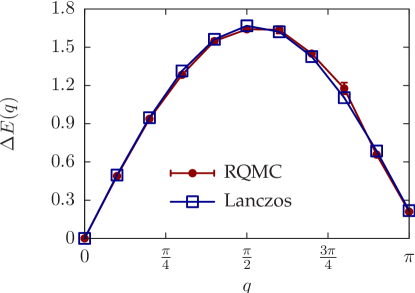
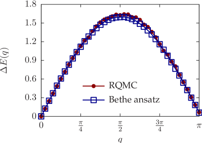
In Fig. 3, we show the results for a small $L=20$ system, where exact diagonalizations are possible by using the Lanczos method. We report the energy excitations $\Delta E(q)=E_{q}-E_{0}$ for the lowest state with $S=1$ and fixed momentum $q$. In this case a perfect agreement between our RQMC results and the exact ones is found. Moreover, also on larger systems a very good accuracy is possible (see Fig. 4), demonstrating the performances of our numerical algorithm.

Figure 5: Ground-state expectation value of the spin-spin correlation function $\mathcal{C}(d)$ for the Heisenberg model on a $80$-site chain.

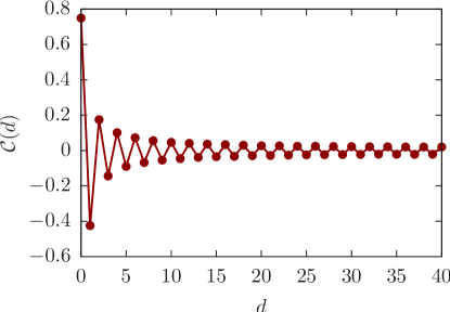
In order to exemplify the potentialities of the scheme outlined in III.3, we conclude this part of the results devoted to the Heisenberg model showing the ground-state expectation value of the spin-spin correlation at distance $d$

$$\mathcal{C}(d) = \frac{1}{L}\sum_{i}\left(\hat{{\bf S}}_{i}\cdot\hat{{\bf S}}_{i+d}\right).$$ (42)

The desired observable is used as a worm operator and the value of the correlation function at the various distances is computed by means of the estimator of Eq. (33). In Fig. 5, we show the expectation value of $\mathcal{C}(d)$ for a $80$-site one-dimensional lattice. In this case we are able to achieve very good statistics for the off-diagonal observable, with a relatively negligible computational effort, when compared to the evaluation of the ground-state expectation value of other diagonal observables.

IV.2 Ground-state properties of the fermionic Hubbard model

As an example of the application of the RQMC to sign-problem affected Hamiltonians, we present some results for the fermionic Hubbard model on a square lattice, defined by:

$$\hat{H}=-t\sum_{\langle i,j\rangle,\sigma}\hat{c}_{i,\sigma}^{\dagger}\hat{c}_{j,\sigma}+h.c.+U\sum_{i}\hat{n}_{i,\uparrow}\hat{n}_{i,\downarrow},$$ (43)

where $\langle\dots\rangle$ indicate nearest-neighbor sites, $\hat{c}_{i,\sigma}^{\dagger}$ ($\hat{c}_{i,\sigma}$) creates (destroys) an electron on the site $i$ with spin $\sigma$, and $\hat{n}_{i,\sigma}=\hat{c}_{i,\sigma}^{\dagger}\hat{c}_{i,\sigma}$. As a variational state we consider

$$|\Psi_{V}\rangle=\exp\left[\sum_{i,j}v_{ij}\hat{n}_{i}\hat{n}_{j}\right]|FS\rangle$$ (44)

where $|FS\rangle$ is the non-interacting Fermi sea and the Jastrow factor involves density-density correlations. The variational parameters $v_{ij}$ entering in the Jastrow factor may be optimized again by minimizing the variational energy with the method of Ref. Sorella:2005, . In order to avoid open shells in $|FS\rangle$, we consider $45$-degrees tilted lattices with $L=2\times l^{2}$ sites, such that both the half-filled case and selected holes-doped cases are closed shells.

Figure 6: Ground-state energy for the fermionic Hubbard model at half filling on a $18$-sites tilted-square lattice. The energy difference $\Delta E=E_{\text{exact}}-E$ is computed with distinct approximations described in the text.

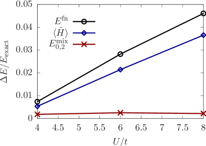
Let us start by showing the results for $18$ electrons on $18$ sites, where Lanczos diagonalizations are possible. Becca:2000 In Fig. 6, we report our results for the ground-state energy. The FN approach gives rather accurate results for small values of $U/t$, i.e., $U/t\lesssim 4$, where $(E_{\text{exact}}-E^{\text{fn}})/E_{\text{exact}}\lesssim 0.01$. By increasing the on-site interaction, the FN approach becomes worse and worse. This fact is due to the choice of the variational wave function that does not contain antiferromagnetic order. Remarkably, a considerable improvement may be obtained by considering the pure expectation value of the Hamiltonian, which is systematically lower than the FN energy, as demonstrated in Ref. CeperleyFN, and now accessible within our algorithm. Further improvements to the FN energy can be obtained upon considering few (up to three) higher moments of the Hamiltonian measured as mixed-averages, see Fig. 6. The scheme based upon the Hamiltonian moments (described in Sec. III.4) allows us to reach a great accuracy for the ground state energy, with a residual error almost independent of $U/t$. Indeed, in this way we have $(E_{\text{exact}}-E)/E_{\text{exact}}\lesssim 0.002$ up to $U/t=8$.

This approach remains very effective also for larger systems, even though the variational wave function loses accuracy by increasing the cluster size (because the ground state has antiferromagnetic order in the thermodynamic limit, while the variational state is paramagnetic). In Table 1, we report the ground-state energy for $50$ sites for the half-filled case, while in Table 2 we report the ground-state energies for selected cases at finite hole-doping, where numerically exact results (for moderate values of $U$ and moderate lattice sizes) can be obtained by the Auxiliary-Field Monte Carlo method. SorellaPriv

$U/t$	$E^{\text{fn}}$	$\langle\hat{H}\rangle$	$E_{0,2}^{\text{mix}}$
$4$	$-42.850(1)$	$-43.16(1)$	$-43.282(1)$
$5$	$-36.364(1)$	$-36.51(1)$	$-37.052(1)$
$6$	$-31.885(1)$	$-32.17(1)$	$-32.640(1)$
$7$	$-28.318(1)$	$-28.66(1)$	$-29.022(1)$
$8$	$-25.382(1)$	$-25.62(1)$	$-26.056(1)$

Table 1: Ground-state energy as a function of the Hubbard $U$ repulsion on the $50$-site lattice at half filling.

$N$	$E^{\text{fn}}$	$\langle\hat{H}\rangle$	$E_{0,2}^{\text{mix}}$	$E_{AF}$
$50$	$-42.850(1)$	$-43.16(1)$	$-43.282(1)$	$-43.983(1)$
$42$	$-53.402(1)$	$-53.57(1)$	$-53.769(1)$	$-54.001(1)$
$26$	$-55.4325(1)$	$-55.63(1)$	$-55.6112(1)$	$-55.782(1)$
$18$	$-50.4127(1)$	$-50.50(1)$	$-50.4383(1)$	$-50.474(1)$

Table 2: Ground-state energy as a function of the number of electrons $N$ for Hubbard repulsion $U/t=4$ on a $50$-site lattice. The numerically exact results obtained by the Auxiliary-Field Monte Carlo method $E_{AF}$ are also shown for comparison. SorellaPriv

V Conclusions

In this paper we have provided an efficient and general formulation of the reptation quantum Monte Carlo technique on lattice models. In particular, we showed an alternative sampling approach which generalizes the bounce algorithm, previously introduced to reduce auto-correlation time of the observables. Our scheme allows one to choose the time direction in a purely Markovian way. In addition, the average number of consecutive moves along the time directions may be optimized by a fine tuning of a certain parameter that has been expressly introduced in the transition probabilities. We reported benchmarks for two different models with pure bosonic and fermionic degrees of freedom, by showing to what extent it is possible to have accurate results both on the ground state and low-energy excitations. The introduction of a general method to compute ground-state expectation values of arbitrary off-diagonal observables also constitutes an important achievement, which will ease the study of relevant properties such as Bose-Einstein condensation and superconductivity phenomena in strongly interacting models. In addition, the possibility to directly measure the pure ground-state expectation values may open the way to a better optimization of the correlated wave function associated to the ground-state of an effective Hamiltonian which is not the FN one.

Appendix A Derivation of the probabilities for the directed-update scheme

In this Appendix we give a detailed derivation of the probabilities for the directed updates. The detailed balance condition guarantees that the given probability distribution $\Pi^{\beta}(\mathbf{X})$ is sampled if transitions from an initial state $\mathbf{X}^{k}$ to a final state $\mathbf{X}^{k+s}$ differing for $s$ intermediate updates are accepted according to:

$$A^{s}=\min\left\{1,\frac{\Pi^{\beta}(\mathbf{X}^{k+s})}{\Pi^{\beta}(\mathbf{X}^{k})}\frac{\mathcal{T}^{s}(\mathbf{X}^{k+s}\rightarrow\mathbf{X}^{k})}{\mathcal{T}^{s}(\mathbf{X}^{k}\rightarrow\mathbf{X}^{k+s})}\right\},$$ (45)

$\mathcal{T}^{s}$ being the overall transition probability between the two states. Let us first consider the case when $s=1$ and fix the right direction $d=R$ (a similar derivation can be obtained for $d=L$). In this case, the transition probability from the initial state to the final state reads

$$\mathcal{T}^{1}(\mathbf{X}^{k}\rightarrow\mathbf{X}^{k+1}) = P(\mathbf{X}^{k},\rightarrow)\times R^{\tau}(x_{2M}^{k}\rightarrow x_{2M}^{k+1})\times$$ (46)

$$\times \left[1-K(\mathbf{X}^{k+1},\rightarrow)\right],$$

namely, it is the product of the probability of having chosen the right direction, times the transition probability for the new tail of the reptile, times the probability of stopping the updates after one intermediate step. The inverse transition probability instead reads

$$\mathcal{T}^{1}(\mathbf{X}^{k+1}\rightarrow\mathbf{X}^{k}) = P(\mathbf{X}^{k+1},\leftarrow)\times R^{\tau}(x_{0}^{k+1}\rightarrow x_{0}^{k})\times$$ (47)

$$\times \left[1-K(\mathbf{X}^{k},\leftarrow)\right],$$

which can be obtained reversing the time directions and considering transitions from the head of the reptile instead that from the tail. Therefore, the acceptance factor reads as

$$A^{1} = \min\left\{1,\frac{1-K(\mathbf{X}^{k},\leftarrow)}{P(\mathbf{X}^{k},\rightarrow)}\times\right.$$ (48)

$$\left.\times\frac{w(x_{2M-1}^{k+1})}{w(x_{1}^{k})}\times\frac{P(\mathbf{X}^{k+1},\leftarrow)}{1-K(\mathbf{X}^{k+1},\rightarrow)}\right\}.$$

For two intermediate transitions instead the transition probabilities are

$$\mathcal{T}^{2}(\mathbf{X}^{k}\rightarrow\mathbf{X}^{k+2}) = P(\mathbf{X}^{k},\rightarrow)\times R^{\tau}(x_{2M}^{k}\rightarrow x_{2M}^{k+1})\times$$ (49)

$$\times K(\mathbf{X}^{k+1},\rightarrow)\times R^{\tau}(x_{2M}^{k+1}\rightarrow x_{2M}^{k+2})\times$$

$$\times \left[1-K(\mathbf{X}^{k+2},\rightarrow)\right],$$

and

$$\mathcal{T}^{2}(\mathbf{X}^{k+2}\rightarrow\mathbf{X}^{k}) = P(\mathbf{X}^{k+2},\leftarrow)\times R^{\tau}(x_{0}^{k+2}\rightarrow x_{0}^{k+1})\times$$ (50)

$$\times K(\mathbf{X}^{k+1},\leftarrow)\times R^{\tau}(x_{0}^{k+1}\rightarrow x_{0}^{k})\times$$

$$\times \left[1-K(\mathbf{X}^{k},\leftarrow)\right],$$

leading to the acceptance factor

$$A^{2}=\min\left\{1,\frac{1-K(\mathbf{X}^{k},\leftarrow)}{P(\mathbf{X}^{k},\rightarrow)}\times\frac{K(\mathbf{X}^{k+1},\leftarrow)}{K(\mathbf{X}^{k+1},\rightarrow)}\times\right.$$

$$\left.\times\frac{w(x_{2M-1}^{k+1})}{w(x_{1}^{k+1})}\times\frac{P(\mathbf{X}^{k+2},\leftarrow)}{1-K(\mathbf{X}^{k+2},\rightarrow)}\times\frac{w(x_{2M-1}^{k+2})}{w(x_{1}^{k})}\right\}$$ . (51)

The generalization to generic $s$ intermediate steps is straightforward and can be written as

$$A^{s}=\min\left\{1,\frac{1-K(\mathbf{X}^{k},\leftarrow)}{P(\mathbf{X}^{k},\rightarrow)}\times\frac{P(\mathbf{X}^{k+s},\leftarrow)}{1-K(\mathbf{X}^{k+s},\rightarrow)}\times\right.\\ \left.\times\frac{w(x_{2M-1}^{k+s})}{w(x_{1}^{k})}\times\left[{\displaystyle\prod_{l=1}^{s-1}\frac{K(\mathbf{X}^{k+l},\leftarrow)}{K(\mathbf{X}^{k+l},\rightarrow)}\times\frac{w(x_{2M-1}^{k+l})}{w(x_{1}^{k+l})}}\right]\right\}.$$ (52)

To find a simple solution for the unknown probabilities, we first impose a cancellation for the intermediate acceptance factors, namely

$$\frac{K(\mathbf{X},\leftarrow)}{K(\mathbf{X},\rightarrow)}=\frac{w(x_{1})}{w(x_{2M-1})},$$ (53)

this condition is satisfied by Eqs. (19) and (20). Then, we notice that the acceptance factor can be written only in terms of the final and the initial states as

$$A^{s}=\min\left\{1,\frac{q(\mathbf{X}^{k+s},\leftarrow)}{q(\mathbf{X}^{k},\rightarrow)}\right\}.$$ (54)

Further, we can impose the two factors $q$ to be independent on the direction, i.e., the condition $q(\mathbf{X},\leftarrow)=q(\mathbf{X},\rightarrow)=q(\mathbf{X})$, which is satisfied if

$$\frac{P(\mathbf{X},\leftarrow)}{1-K(\mathbf{X},\rightarrow)} \times w(x_{2M-1})=$$ (55)

$$= \frac{P(\mathbf{x},\rightarrow)}{1-K(\mathbf{x},\leftarrow)}\times w(x_{1}).$$

Since the two time directions are mutually exclusive, it is also true that $P(\mathbf{X},\leftarrow)+P(\mathbf{X},\rightarrow)=1$, which allows us to solve Eq. (55) and obtain Eqs. (16) and (17). The same reasoning can be repeated for the left direction and, due to imposed homogeneity for the probabilities, it can be checked that the detailed balance is satisfied for the left direction too.

Appendix B Bounce algorithm, directed updates, and efficiency

In this Appendix we comment on the relationship between the directed-update scheme and the bounce algorithm. If $\alpha=1$ is taken in Eqs. (19) and (20), then after $s$ updates along the direction $d$, at the end of the Markov step $P(\mathbf{X}^{k+s},d)=0$, i.e., the next Markov step will be taken in the opposite direction, just like the bounce algorithm. Although the two algorithms are similar in this particular limit, there is an important difference which eventually leads to a different computational efficiency. In order to elucidate this point and to show the $\alpha$-dependence of the efficiency of the directed updates, we have done a systematic comparison of the two algorithms.

In particular, we have compared the efficiency of the directed updates with the bounce algorithm for a one-dimensional Heisenberg model. The computational efficiency is generally defined as

$$\mathcal{E}=\frac{1}{\sigma_{O}^{2}T},$$ (56)

where $\sigma_{O}^{2}$ is the square of the statistical error associated to a given observable after a given computational time $T$. In Fig. 7, we show the ratio between the directed-update scheme efficiency over the bounce algorithm efficiency, for the measurement of the ground-state energy of a one-dimensional chain.

Figure 7: Relative efficiency of the directed update scheme and the bounce algorithm. The measured quantity is the ground-state energy of the one-dimensional Heisenberg model on a chain of size $L=80$ sites.

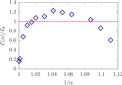
We notice that the two sampling schemes have comparable performances, being both based on a similar approach. As anticipated, it clearly emerges from Fig. 7 that the two algorithms do not have exactly the same behavior at $\alpha=1$, the maximum efficiency of the directed updates being reached for lower values of $\alpha$. This feature is due to the fact that when $\alpha$ is very close to its saturation value, then a single Markov step can consist of a conspicuous number of individual “sliding moves”. Even if this situation leads to a fast decorrelation of configurations it also leads to a rarefaction of the possibility to measure the desired observables, which can eventually take place only at the end of the Markov step and not during the individual moves. This leads to a worse efficiency if compared to the bounce algorithm, where measurements can be in principle done after every sliding move.

In conclusion, the performances of the two algorithms are very close, although some advantages may arise from the use of the directed-updates. We further notice that the purely Markovian approach introduced in this paper could be slightly more efficient in cases where the number of rejected configurations by the bounce algorithm is substantial whereas all the generated configurations are accepted in the directed update scheme.

References

- (1) D.M. Ceperley and E.L. Pollock, Phys. Rev. Lett. 56, 351 (1986).
- (2) D.M. Ceperley, Rev. Mod. Phys. 67, 279 (1995).
- (3) N.V. Prokof’ev, B.V. Svistunov, and I.S. Tupitsyn, Phys. Lett. A 238, 253 (1998).
- (4) M. Boninsegni, N. Prokof’ev, and B. Svistunov, Phys. Rev. Lett. 96, 070601 (2006).
- (5) S. Baroni and S. Moroni, Phys. Rev. Lett. 82, 4745 (1999).
- (6) A. Sarsa, K.E. Schmidt, and W.R. Magro, Journal of Chemical Physics 113, 1366 (2000).
- (7) C. Pierleoni and D.M. Ceperley, ChemPhysChem 6, 1872 (2005).
- (8) G. Carleo, S. Moroni, and S. Baroni, Phys. Rev. B 80, 094301 (2009).
- (9) W. Krauth, N. Trivedi, and D. Ceperley, Phys. Rev. Lett. 67, 2307 (1991).
- (10) O.F. Syljuasen, Phys. Rev. B 73, 245105 (2006).
- (11) O.F. Syljuasen and A.W. Sandvik, Phys. Rev. E 66, 046701 (2002).
- (12) V.G. Rousseau, Phys. Rev. E 78, 056707 (2008).
- (13) A.W. Sandvik, Phys. Rev. B 59, R14157 (1999).
- (14) S.M.A. Rombouts, K. Van Houcke, and L. Pollet, Phys. Rev. Lett 96, 180603 (2006)
- (15) S. Sorella and L. Capriotti, Phys. Rev. B 61, 2599 (2000).
- (16) K.H. Schmidt, P. Niyaz, A. Vaught, and M.A. Lee, Phys. Rev. E 71, 016707 (2005).
- (17) D.F.B. ten Haaf, H.J.M. van Bemmel, J.M.J. van Leeuwen, W. van Saarloos, and D.M. Ceperley, Phys. Rev. B 51, 13039 (1995).
- (18) R.R. Whitehead and A. Watt, J. Phys.G: Nucl. Phys. 4, 835 (1978).
- (19) See for example, T. Giamarchi, Quantum Physics in One Dimension (Oxford University Press, Oxford, 2004).
- (20) J.E. Gubernatis, M. Jarrell, R.N. Silver, and D.S. Silvia, Phys. Rev. B 44, 6011 (1991).
- (21) E. Manousakis, Rev. Mod. Phys. 63, 1 (1991).
- (22) F. Franjic and S. Sorella, Prog. Theor. Phys. 97, 399 (1997).
- (23) S. Sorella, Phys. Rev. B 71, 241103 (2005).
- (24) F. Becca, A. Parola, and S. Sorella, Phys. Rev. B 61, 16287(R) (2000).
- (25) S. Sorella, private communication.