Parallel Generation of Massive Scale-Free Graphs

Abstract

One of the biggest huddles faced by researchers studying algorithms for massive graphs is the lack of large input graphs that are essential for the development and test of the graph algorithms. This paper proposes two efficient and highly scalable parallel graph generation algorithms that can produce massive realistic graphs to address this issue. The algorithms, designed to achieve high degree of parallelism by minimizing inter-processor communications, are two of the fastest graph generators which are capable of generating scale-free graphs with billions of vertices and edges. The synthetic graphs generated by the proposed methods possess the most common properties of real complex networks such as power-law degree distribution, small-worldness, and communities-within-communities. Scalability was tested on a large cluster at Lawrence Livermore National Laboratory. In the experiment, we were able to generate a graph with 1 billion vertices and 5 billion edges in less than 13 seconds. To the best of our knowledge, this is the largest synthetic scale-free graph reported in the literature.

1 Introduction

Recent studies have revealed that many real-world graphs belong to a special class of graphs called complex networks (or graphs). Examples of the real-world complex graphs include World-Wide Web [4], Internet [12, 13, 25, 30], electric power grids [31], citation networks [16, 26, 28, 29], telephone call graphs [1], and e-mail network [9]. These graphs typically carry a wealth of valuable information for their respective domains. Therefore, a great deal of research effort has been concentrated on developing algorithms to identify and mine certain knowledge or data of interest from these graphs. For example, algorithms that can find groups of vertices that have strong associations between them (called communities) have been reported [5, 8, 22, 23, 24]. There exist algorithms which, given a template pattern, can find subgraphs that closely match to the input pattern [17]. Such algorithms can play a very important role in detecting certain criminal activities or making critical business decisions.

The real-world complex graphs are typically very large (with millions or more vertices) and their sizes grow over time. Some researchers predict that the size of these graphs will eventually reach $10^{15}$ vertices [15]. The high complexity of the graph algorithms, combined with the large and increasing size of the target graphs, however, makes these applications to be very difficult to apply to large real graphs. Efforts are being made to parallelize these applications [32, 2] and develop efficient out-of-core graph algorithms [27] to cope with the technical challenges.

One of key issues in developing these graph applications is the availability of large input graphs, as these graphs are essential for the developers to develop and test the applications and to measure their scalability and performance. Unfortunately, we do not have publicly available real graphs that are large enough to test the functionality and true scalability of the graph applications. A social network graph derived from the World Wide Web, for example, contains 15 million vertices [11] and the largest citation network available has two million vertices [21]. Although these real-world graphs tend to grow in size, it is unlikely that the real graphs of sufficiently large size will be available in the near future.

The lack of the large graphs has forced the researchers to use synthetically generated random graphs, which are relatively cheap to construct, in their experiments [32]. The random graphs (also known as Erdös-Rényi random graphs [10]), however, is uninformative, since the structure of the random graphs greatly differs from that of real-world graphs. In the absence of the large real graphs, synthetic graphs may be used for the development of the graph applications. There exist several good models to synthetically generate complex networks [3, 18, 31]. A serious drawback of these models is that they are all sequential models and hence, are inadequate to use to generate the massive graphs with billions of vertices and edges.

In this paper, we propose two efficient and highly scalable graph generation methods. Based on serial models [3, 18], these methods are designed to generate massive scale-free graphs in parallel on distributed parallel computers. These parallel generators require very little inter-processor communications and thus achieve high degree of parallelism. The first method, called parallel Barabasi-Albert (PBA) method, iteratively builds a graph using a technique called two-phase preferential attachment. The second parallel method, called parallel Kronecker (PK) method, applies the concept of Kronecker product of matrices [14] and constructs a graph recursively in a fractal fashion from a given seed graph. These are two of the fastest graph generation algorithms with capability of generating scale-free graphs with billions of vertices and edges. We have demonstrated their scalability by constructing massive graphs on a large cluster at Lawrence Livermore National Laboratory. In the experiment, we have generated a scale-free graph with 1 billion vertices and 5 billion edges in less than 13 seconds, and to the best of our knowledge, this is the largest synthetic scale-free graph ever reported in the literature. We also have analyzed the properties of the graphs generated by the proposed methods and report the results in this paper. We have found that these graphs possess commonly known properties of real-world complex networks, including power-law degree distribution, small-worldness, and communities-within-communities.

The remaining of the paper is organized as follows. Section 2 surveys the related work in the literature. The proposed parallel models are described in Section 3. Section 4 presents the results from performance and characterization study, followed by concluding remarks and directions for future work in Section 5.

2 Related Work

Erdös and Rényi have proposed a simple model that generates equilibrium random graphs, called Erdös-Rényi random graphs [10]. In this model, given a fixed number of vertices, a graph is constructed by connecting randomly chosen vertices with an edge repeatedly until the predetermined number of edges are obtained. This model is restrictive in that it produces only Poisson degree distributions.

Dorogovtsev et al. proposed a model that can generate graphs with fat-tailed degree distributions [7]. Given a random graph, this model restructures the given graph by rewiring a randomly chosen end of a randomly chosen edge to a preferentially chosen vertex and also moving a randomly chosen edge to a position between two preferentially chosen vertices at each step of the evolution.

The model proposed by Watts and Strogatz [31] generates random structures with small diameter, which has been named as small-world graphs. This model transforms a regular one-dimensional lattice (with vertex degree of four or higher) by rewiring each edge, with certain probability, to a randomly chosen vertex. It has been found that, even with the small rewiring probability, the average shortest-path length of the resulting graphs is of the order of that of random graphs, and generate graphs with fat-tailed degree distributions.

The majority of recent models uses a method called preferential attachment [6]. In a representative model among these, proposed by Barabasi and Albert [3], a new vertex joins the graph at each time step and gets connected to an existing vertex with probability proportional to the vertex degree. With preferential attachment, these models can emulate the dynamic growth of real graphs.

Leskovec et al. [18] have proposed a graph generation model that addresses some of recently discovered properties of time-evolving graphs: densification and shrinking diameter. The main idea of their model is to recursively create self-similar graphs with certain degree of randomness. The self-similarity of the graphs is achieved by using the Kronecker product (also known as tensor product) [14], which is a natural tool to construct self-similar structures. Given a seed graph, at each step this model computes the Kronecker product of two matrices that represent the seed graph and the graph generated in previous step respectively. The graphs generated with this method have regular structure. The model changes the entries in the target matrix with a certain probability before each multiplication to add randomness to the graph.

3 Proposed Graph Generation Methods

Parallel Barabasi-Albert (PBA) method

Scale-free graphs can be easily generated using a well-known technique called preferential attachment [6]. In a simple serial model known as Barabasi-Albert (BA) model [3], a scale-free graph is constructed, starting with a small clique, by repeatedly creating a vertex and attach it to one of the existing vertices with probability proportional to its current degree.

We have parallelized the BA model in this research and propose a graph generation algorithm called parallel BA (PBA) method. In this method, vertices are distributed to the processors, and all the edges adjacent to a given vertex are stored on the same processor to which the vertex is assigned.

Sets of processors called factions are used in the PBA method. Each processor belongs to one or more factions. The number of processors in each faction varies. Such variation is essential for the correct implementation of the preferential attachment operation in a distributed environment. Furthermore, we can assign the processors to factions in a manner to enable us to generate graphs with certain structures. The size of each faction is a degree of freedom in this method. The number of factions is another degree of freedom. To facilitate the implementation, we choose to assign all vertices on a single processor to the same set of factions. In other words, if two vertices reside on the same processor, then they are members of the same set of factions.

It is crucial to use an efficient implementation of the preferential attachment to allow this method to scale. This can be done most efficiently by selecting an existing edge from the graph with a uniform probability and then randomly selecting one of its endpoints as the point to which a new vertex can be attached. Therefore, an edge can be added in constant time in this implementation.

A slight variation of this algorithm is used in the PBA method. The proposed PBA algorithm is described below in detail. It is assumed that the algorithm runs on a processor $p$. Other processors perform the same algorithm. We also assume that $p$ is a member of factions $F_{0}$, $F_{1}$, …, $F_{n-1}$.

In the PBA method, an edge is attached in two phases. In the first phase of our preferential attachment, $k$ edges are added per newly created local vertex (a vertex that resides on $p$) as in the conventional BA model. However, each edge, $e$, associates a local vertex with some processor $q$, instead of connecting two vertices as in the serial model. The particular vertex that is to be the eventual endpoint of $e$ is determined remotely by the processor $q$.

The processor $q$ is selected using a variation of the preferential attachment algorithm as follows. Let $A$ denote a local edge list maintained by the processor $p$. First, we initialize $A$ by associating the first $s$ edges with the processors in factions $F_{0}$, $F_{1}$, …, $F_{n-1}$, matching sequentially one edge to one processor in the set of factions. Here, $s$ is the total number of processors in factions $F_{0}$, $F_{1}$, …, $F_{n-1}$ (i.e., $s=\sum_{i=0}^{n-1}|F_{i}|$). For an edge $e_{j}$, where $j\geq s$, we select an existing edge from $A$ with a uniform probability (thus realizing preferential attachment) and then assign its associated processor to $e_{j}$. This process is repeated until the predetermined number of local vertices and edges are created on $p$. At the end of the first phase, $p$ sends a message to each processor $q$ to notify the number of occurrences of $q$ in $A$.

In the second phase, $p$ determines the endpoints for the edges on remote processors and connects the endpoints calculated by remote processors to its local vertices. The processor $p$ first receives messages from other processors, which contain the numbers of occurrences of $p$ in their respective local edge list. That is, the message received from a processor $q$ represents the number of incomplete edges one of whose endpoints resides on the processor $q$. These edges are to be connected to the local vertices on $p$, selected by using the standard preferential attachment technique. Once the list of the vertices for the attachment is determined, it is divided up among the processors. Here, each processor is assigned as many vertices as it requested. The selected vertices are then sent to the corresponding processors.

Having sent the endpoints for the remote edges, then $p$ receives the lists of endpoints from other processors for its own incomplete edges. Using the remote vertices received, $p$ completes its local partition of the graph. This is done by simply substituting each occurrence of processor $q$ in $A$ with the next endpoint in the list sent by $q$. The resulting collection of edges defines the portion of the graph stored on $p$.

$u$ 0 0 1 1 2 2 3 3 4 4 $v$ $P_{1}$ $P_{2}$ $P_{0}$ $P_{1}$ $P_{1}$ $P_{2}$ $P_{0}$ $P_{1}$ $P_{0}$ $P_{2}$

(a) Edge list on $P_{0}$ at the end of phase 1

$u$ 0 0 1 1 2 2 3 3 4 4 $v$ 8 $P_{2}$ $P_{0}$ 7 5 $P_{2}$ $P_{0}$ 8 $P_{0}$ $P_{2}$

(b) A snapshot of edge list on $P_{0}$ during the phase 2

Figure 1: An example of PBA graph construction on processor $P_{0}$. A list of edges, ($u$, $v$) is maintained on $P_{0}$, where $u$ denotes a local vertex and $v$ is an endpoint determined by remote processors in phase 2. In this example, three factions are used, where $F_{0}$ = {$P_{1}$, $P_{2}$}, $F_{1}$ = {$P_{1}$, $P_{3}$}, $F_{2}$ = {$P_{0}$, $P_{1}$}. Processor $P_{0}$ belongs to fractions $F_{0}$ and $F_{2}$.

The two-phase preferential attachment is explained using an example in Figure 1. In this example, we generate a graph with 5 vertices per processor and 2 edges per vertex. It is assumed that there are three factions, $F_{0}$ = {$P_{1}$, $P_{2}$}, $F_{1}$ = {$P_{1}$, $P_{3}$}, and $F_{2}$ = {$P_{0}$, $P_{1}$} and processor $P_{0}$ belongs to fractions $F_{0}$ and $F_{2}$. The vertices are assumed to be evenly distributed among the processors so that vertices 0–4 are on $P_{0}$, vertices 5–8 on $P_{1}$, and so on.

In the first phase of the algorithm, $P_{0}$ selects processors and associates them with the local vertices as shown in Figure 1.a, where the edge list on $P_{0}$ is depicted. Note that the first four processors in the list are the ones in the factions that $P_{0}$ belongs to, $F_{0}$ and $F_{2}$. The rest of the processors in the list are selected using the standard preferential attachment technique. At the end of phase 1, $P_{0}$ needs four endpoints from $P_{1}$ (and three endpoints from each of $P_{0}$ and $P_{2}$). These endpoints are determined by processor $P_{1}$ via preferential attachment and sent to $P_{0}$ in the second phase. In this example, we assume that vertices 8, 7, 5, and 8 are sent to $P_{0}$. Once receiving the list, $P_{0}$ simply replaces the entries marked with $P_{1}$ with the endpoints in the list. This is shown in Figure 1.b.

We have found that it is useful to modify the algorithm slightly to incorporate some inter-faction edges. In particular, during the first phase, we occasionally select a processor that is not in any of the factions of $p$. Such processors are chosen randomly. The probability of creating an inter-faction edge is an another degree of freedom in this algorithm.

Parallel Kronecker (PK) method

	$\left(\begin{array}[]{ccccc}1&1&1&1&0\\ 1&1&0&0&0\\ 1&0&1&0&0\\ 1&0&0&1&0\\ 0&0&0&0&1\\ \end{array}\right)$
(a) Seed graph $G_{1}$ with 5 vertices	(b) Adjacency matrix for $G_{1}$

$\left(\begin{array}[]{ccccc}G_{1}&G_{1}&G_{1}&G_{1}&0\\ G_{1}&G_{1}&0&0&0\\ G_{1}&0&G_{1}&0&0\\ G_{1}&0&0&G_{1}&0\\ 0&0&0&0&G_{1}\\ \end{array}\right)$
(c) Adjacency matrix for $G_{2}=G_{1}\otimes G_{1}$	(d) Plot for $G_{4}$

Figure 2: An example of the Kronecker multiplication for graph generation. $G_{2}$ is constructed by multiplying the seed graph with itself (that is, $G_{2}=G_{1}\otimes G_{1}$). The self-similarity in $G_{4}$ is clearly shown in (d).

A model that uses well-known concept of Kronecker matrix multiplication to generate scale-free graphs has been recently proposed [18]. If $A$ is an $m\times n$ matrix and $B$ is a $p\times q$ matrix, then the Kronecker product $A\otimes B$ is the $mp\times nq$ block matrix, defined as

$$A\otimes B=\left(\begin{array}[]{ccc}a_{11}B&\cdots,&a_{1n}B\\ \vdots&\ddots&\vdots\\ a_{m1}B&\cdots,&a_{mn}B\end{array}\right)~{}\cite[cite]{[\@@bibref{}{horn1991}{}{}]}.$$

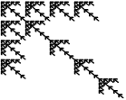
The Kronecker product of two graphs is defined as the Kronecker product of their adjacency matrices. Figure 2 shows an example where a Kronecker graph is generated from given seed graph using the Kronecker graph multiplication. Since the Kronecker method is an ideal tool to construct self-similar structures, the graph generated by this method has also self-similar structure as shown in Figure 2.d.

Implementing a serial algorithm for the above graph generation method is straightforward. Starting with an $n_{0}\times n_{0}$ adjacency matrix with $e_{0}$ edges representing a given seed graph, we recursively construct larger adjacency matrices using Kronecker matrix multiplication in a top-down manner. To generate the $i_{th}$ matrix from the $(i-1)_{th}$ matrix, we simply replace every 1 in the $i_{th}$ matrix by an $n_{0}\times n_{0}$ block that is a copy of the seed graph. We replace every 0 by an $n_{0}\times n_{0}$ block of zeros. So if the $i_{th}$ graph has $n_{i}$ vertices, the $(i+1)_{th}$ graph has $n_{i}\times n_{i}$ vertices. Thus, $n_{i}$ = $n_{0}^{i+1}$ for all iterations. We treat each edge in the graph at each iteration as a meta-edge. A meta-edge is defined by its iteration and its position in the graph for that particular iteration. Given the size of a target graph, we can calculate the number of iterations required to generate the target graph.

A Kronecker graph can be generated efficiently by using a stack, initialized with the edges in the seed graph. A graph is generated by expanding meta-edges in the stack as follows. First, a meta-edge on the top of the stack is popped up. If its iteration, $i$, is equal to the predetermined final iteration, then the edge is added to the final graph. Otherwise, new meta-edges with iteration $i+1$ are generated and pushed onto the stack. This operation is repeated until the stack is depleted. We choose a stack because it guarantees that the memory requirement is limited to $O(\sqrt[e_{0}]{|E|})$, where $|E|$ is the number of edges in the final graph. An implementation using a queue is not scalable, as it would require $O(|E|)$ memory space.

In the parallel implementation of the Kronecker method, the meta-edges are divided among the groups of processors at each iteration. Each processor group generates the same meta-edges at a given iteration. If there are more processors in a processor group than there are edges in that group’s portion of the graph, then each processor in the group is assigned to a single edge in the stack. Here, each edge defines a new processor group that is a subset of the original, and the process group ignores all other meta-edges at that iteration. On the other hand, if there are more meta-edges than processors in the processor group, the edges are divided as evenly as possible among those processors. Each of those processors is then in a singleton processor group for the remaining iterations. Each processor must be able to calculate on the fly which meta-edges are in its processor group at a given iteration.

In general, it is difficult to achieve good load balance with the PK method, as some processors may be assigned more work depending on processor group sizes. A dynamic load balancing scheme may be used in conjunction with the PK method to overcome this limitation. Furthermore, some randomization logics are needed to irregulate the structure of the PK graphs. One approach for the randomization is to add or delete meta-edges during the replacement phase at each iteration by randomly modifying the seed graph temporarily. Another approach is to perform exclusive-OR operation between the final adjacency matrix with the adjacency matrix for a random graph.

4 Experimental Results

4.1 Experiment environment and metrics of interest

We have conducted a study to evaluate the proposed graph generators. The experiments were conducted on MCR [20], a large Linux cluster located at Lawrence Livermore National Laboratory. MCR has 1,152 nodes interconnected with a Quadrics switch, and each of the compute nodes has two 2.4 GHz Intel Pentium 4 Xeon processors and 4 GB of memory,

In this study, we are mainly interested in evaluating the performance of the proposed graph generators and analyzing the graphs they generate. There are well-known structural and temporal properties of the real complex networks [19]. We use widely-accepted properties as indices to quantitatively evaluate the synthetic graph generated by the proposed methods.

4.2 Results

Methods	$|V|$ (Million)	$|E|$ (Billion)	Time (Seconds)
PBA	1,000	5	12.39
PK	0.53	5.4	2.53

Table 1: Comparison of graph generation time by PBA and PK methods. The number of vertices and edges in generated graphs are denoted by $|V|$ and $|E|$, respectively.

Two graphs were generated by using the PBA and PK methods on 1,000 processors on the MCR cluster, and we report the graph generation times in Table 1. The generation time is an average of multiple runs. We have measured the maximum time across all processes in each run. The disk I/O time is not included in the time reported.

Both graphs have about 5 billion edges. The number of vertices in the PK graph is considerably smaller than that in the PBA graph due to our use of a seed graph with large average degree. As shown in the table, it takes less than 13 seconds to generate these massive graphs. The high generation rate can be attributed to the high degree of parallelism of the proposed algorithms.

Figure 3: Weak-scaling results

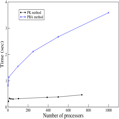The performance of both methods is further detailed in Figure 3, where we show the results from a weak-scaling study. In a weak-scaling test, the global problem size increases as the total number of processors increases such that the size of local problem remains constant. The local problem size of roughly one million vertices and three million edges is used. The figure reveals that the PK method is about four times faster than the PBA method. In particular, the almost flat curve for the PK method highlights the embarrassingly-parallel nature of the algorithm. The graph generation time for the PBA method, on the other hand, increases as the number of processors increases. This is because in the PBA method each processor processes endpoint vertices sent by remote processors at the end of the execution, and the complexity of the processing increases in proportion to the total number of processors used. Profiling of the code confirms that each process spends most of its time in processing the received endpoints.

(a) PBA graph ($\gamma=2.75$)	(b) PK graph ($\gamma=2.47$)

(c) Router graph ($\gamma=2.19$)

Figure 4: Degree distributions of the synthetic and router graphs. Here $k$ and $P(k)$ denote the degree and the number of vertices with degree $k$, respectively. The $\gamma$ exponent of a power-law distribution, $P(k)\propto k^{-\gamma}$, for each graph is obtained through curve fittings and shown here as well.

In the remaining of this section, we analyze the graphs produced by the proposed methods. A PBA graph studied in this experiments has 330,000 vertices and 2 million edges. A PK graph with 160,000 vertices and 28 million edges, constructed using a small seed graph with 20 vertices and 40 edges, is analyzed. We also consider two real-world graphs, WWW and router graphs, for comparison. The WWW graph has 325,000 vertices and 2.1 million edges, and the smaller router graph has 285,000 vertices and 861,000 edges.

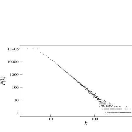
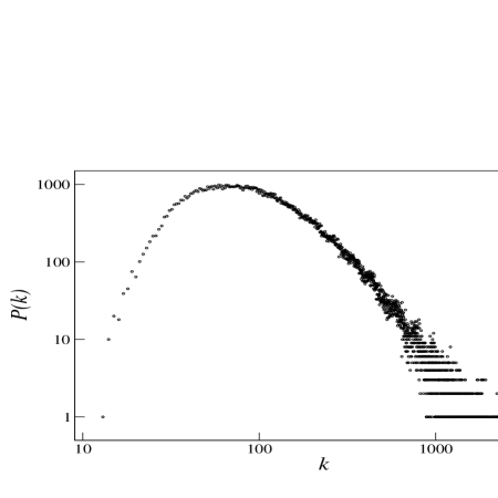
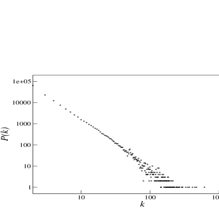
Figure 4 presents the degree distributions of the synthetic graphs and compares them with that of the router graph. The graphs are shown in a log-log scale. As shown in the figure, the curves for both PBA and PK graphs are heavy-tailed. This is a signature of power-law degree distribution that is one of the widely accepted property of real-world complex networks. It is shown in Figure 4.c that the router graph also has fat-tailed degree distribution. To verify that these graphs have power-law degree distributions, $P(k)\propto k^{-\gamma}$, we have performed curve fittings for the measured degree distributions and show the exponent of the power-law distribution ($\gamma$) in Figure 4. As shown in the figure, $\gamma$ values for the three graphs are greater than 2. This finding coincides with the fact that if the average degree of a scale-free graph is finite, then its $\gamma$ value should be $2<\gamma<\infty$ [6]. The PK graph has a large number of high degree vertices. This is because the number of low-degree vertices is small in a graph generated by the PK method, in which the degree of a vertex grows exponentially. We can change the degree distribution by randomly adding low-degree vertices to the final graph.

Graph	Avg. Path Length	Diameter (estimated)
WWW Graph	7.54	46
Router Graph	8.87	27
PK Graph	3.20	5
PBA Graph	6.26	12

Table 2: The comparison of path length and diameter of the synthetic graphs with two real graphs. Both metrics are estimated by sampling to reduce the computation overhead.

Table 2 presents the average path lengths and diameters of the two synthetic graphs considered in the previous experiment as well as the WWW and router graphs. Both metrics are estimates obtained through sampling to reduce the computation time. Each of the graphs analyzed has short average path length, which is the average value of the shorted path between two randomly chosen vertices. Further, each synthetic graph has a small diameter that is the maximum of all-pairs shortest path. These results indicate that the graphs generated by the proposed methods have small world property, which is another key characteristic of real-world complex networks. Obviously, such small-worldness is more evident in the PK graph, as it contains a large number of high-degree vertices (or hubs). Two real graphs, the WWW graph in particular, appear to have the smaller number of hubs as indicated by the larger diameters.

(a) PBA graph	(b) PK graph

Figure 5: Communities within PBA and PK graphs. The graphs are represented as adjacency matrices.

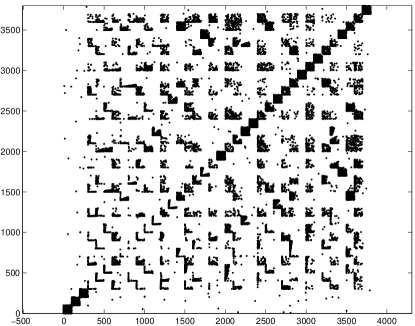
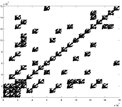
In Figure 5, we show two adjacency matrices for PBA and PK graphs to visualize the community structures within these synthetic graphs. As shown in the figure, the PBA and PK graphs have clearly identifiable community structures. A major difference between the two graphs is that the PK graph has more regularly-structured communities compared to the PBA graph. The regular community structure of the PK graph is the result of the systematic way of graph construction by the PK method (using the Kronecker matrix multiplication). In addition, the self-similar nature of the Kronecker product is translated into the communities-within-communities structure in the PK graph.

4.3 Comparison of the PBA and PK methods

An advantage of the PK method over the PBA method is its higher degree of parallelism. The PK method is embarrassingly parallel, as once a seed graph is given, processors generate the assigned portions of the target graph independent of each other. A key limitation of the PK method is that the structure of a resulting graph heavily depends on that of the initial seed graph. In fact, even with randomized edge generation and removal, the structure of final graph largely depends on the seed graph and thus relatively regular. In consequence, this limitation makes it very difficult to configure the PK method to generate a graph with desired property. For example, if the seed graph is too small it is very difficult to control the degree of vertices. To control the vertex degree, we need a relatively large seed graph, but with such a large seed graph, it is hard to control the size of the final graph.

Although slower than the PK method, the PBA method is still a very fast algorithm. An obvious advantage of the PBA method is that using preferential attachment as a key means to construct a graph, the method can be easily configured to generate a graph of desired size and properties.

5 Conclusions and Future Work

Two efficient and scalable parallel graph generation methods that can generate scale-free graphs with billions of vertices and edges are proposed in this paper. The proposed parallel Barabasi-Albert (PBA) method iteratively builds scale-free graphs using two-phase preferential attachment technique in a bottom-up fashion. The parallel Kronecker (PK) method, on the other hand, constructs a graph recursively in a top-down fashion from a given seed graph using Kronecker matrix multiplication. These parallel graph generators operate with high degree of parallelism. We have generated a graph with 1 billion vertices and 5 billion edges in less than 13 seconds on a large cluster. This is the highest rate of graph generation reported in the literature. We have analyzed the graphs produced by our methods and shown that they have the most common properties of the real complex networks such as power-law degree distribution, small-worldness, and communities-within-communities.

There are other known and somewhat debatable properties of complex networks. A rigorous study of the graphs generated by the proposed methods will reveal whether these methods can produce synthetic graphs with these properties. This study will also provide us with better understanding of how the logics used in our algorithms affect the properties of the synthetic graphs they generate. Based on this study, we will develop a set of pre- and post-generation processing and randomization techniques that will enable us to construct a synthetic graph with desired properties.

References

- [1] W. Aiello, F. Chung, and L. Lu. A random graph model for massive graphs. In Proceedings of the thirty-second annual ACM symposium on Theory of computing (STOC ’00), pages 171–180, New York, NY, USA, 2000.
- [2] D. A. Bader and K. Madduri. Designing multithreaded algorithms for breadth-first search and st-connectivity on the cray mta-2. In Proceedings of International Conference on Parallel Processing (ICPP 2006), Aug. 2006.
- [3] A.-L. Barabasi and R. Albert. Emergence of scaling in random networks. Science, 286:509, 1999.
- [4] A. Broder, R. Kumar, F. Maghoul, P. Raghavan, S. Rajagopalan, R. Stata, and A. Tomkins. Graph structure in the web: Experiments and models. In 9th World Wide Web Conference, 2000.
- [5] A. Clauset, M. E. J. Newman, and C. Moore. Finding community structure in very large networks. Phys. Rev. E, 70(6):066111, Dec. 2004.
- [6] S. N. Dorogovtsev and J. F. F. Mendes. Evolution of Networks. Oxford University Press, 2004.
- [7] S. N. Dorogovtsev, J. F. F. Mendes, and A. N. Samukhin. Principles of statistical mechanics of random networks. Nuclear Physics B, 666:396, 2003.
- [8] J. Duch and A. Arenas. Community detection in complex networks using extremal optimization. Physical Review E, 72:027104, Jan. 2005.
- [9] H. Ebel, L.-I. Mielsch, and S. Bornholdt. Scale-free topology of e-mail networks. Physical Review E, 66:035103, 2002.
- [10] P. Erdös and A. Rényi. On random graphs. Publ. Math. Debrecen, 6:290–297, 1959.
- [11] C. Faloutsos, K. McCurley, and A. Tomkins. Fast discovery of connection subgraphs. In Proceedings of the 10th ACM SIGKDD International Conference on Knowledge Discovery and Data Mining, pages 118–127, Seattle, WA, USA, 2004.
- [12] M. Faloutsos, P. Faloutsos, and C. Faloutsos. On power-law relationships of the internet topology. In SIGCOMM, pages 251–262, 1999.
- [13] R. Govindan and H. Tangmunarunkit. Heuristics for internet map discovery. In IEEE INFOCOM 2000, pages 1371–1380, Tel Aviv, Israel, March 2000.
- [14] R. Horn and C. Johnson. Topics in Matrix Analysis. Cambridge University Press, 1991.
- [15] T. Kolda, D. Brown, J. Corones, T. Critchlow, T. Eliassi-Rad, L. G. andBruce Hendrickson, V. Kumar, D. Lambert, C. Matarazzo, K. McCurley, M. Merrill, N. Samatova, D. Speck, R. Srikant, J. Thomas, M. Wertheimer, and P. C. Wong. Data sciences technology for homeland security information management and knowledge discovery, 2004. Report of the DHS Workshop on Data Sciences.
- [16] P. L. Krapivsky, S. Redner, and F. Leyvraz. Connectivity of growing random networks. Physical Review Letters, 85:4629, 2000.
- [17] M. Kuramochi and G. Karypis. Frequent subgraph discovery. In Proceedings of the 2001 IEEE International Conference on Data Mining (ICDM ’01), pages 313–320, Washington, DC, USA, 2001.
- [18] J. Leskovec, D. Chakrabarti, J. Kleinberg, and C. Faloutsos. Mathematically tractable graph generation and evolution, using kronecker multiplication. In Proceedings of European Conference on Principles and Practice of Knowledge Discovery in Databases, 2005.
- [19] J. Leskovec, J. Kleinberg, and C. Faloutsos. Graphs over time: densification laws, shrinking diameters and possible explanations. In Proceeding of the eleventh ACM SIGKDD international conference on Knowledge discovery in data mining (KDD ’05), pages 177–187, 2005.
- [20] Multiprogrammatic Capability Cluster (MCR). http://www.llnl.gov/linux/mcr.
- [21] M. E. J. Newman. From the cover: The structure of scientific collaboration networks. Proceedings of the National Academy of Sciences, 98:404–409, 2001.
- [22] M. E. J. Newman. Detecting community structure in networks. European Physical Journal B, 38:321–330, May 2004.
- [23] M. E. J. Newman. Fast algorithm for detecting community structure in networks. Phys. Rev. E, 69(6):066133, June 2004.
- [24] M. E. J. Newman and M. Girvan. Finding and evaluating community structure in networks. Phys. Rev. E, 69(2):026113, Feb. 2004.
- [25] R. Pastor-Satorras, A. Vazquez, and A. Vespignani. Dynamical and correlation properties of the internet. Physical Review Letters, 87:258701, 2001.
- [26] S. Redner. How popular is your paper? an empirical study of the citation distribution. The European Physical Journal B, 4:131, 1998.
- [27] J. F. Sibeyn, J. Abello, and U. Meyer. Heuristics for semi_external depth first search on directed graphs. In Proceedings of the ACM Symposium on Parallel Algorithms and Architectures, (SPAA’02), pages 282–292, 2002.
- [28] C. Tsallis and M. P. de Albuquerque. Are citations of scientific papers a case of nonextensivity? The European Physical Journal B, 13:777, 2000.
- [29] A. Vazquez. Statistics of citation networks, 2001. cond-mat/0105031.
- [30] A. Vazquez, R. Pastor-Satorras, and A. Vespignani. Large-scale topological and dynamical properties of internet. Physical Review E, 65:066130, 2002.
- [31] D. J. Watts and S. H. Strogatz. Collective dynamics of small-world networks. Nature, 393:440–442, 4 June 1998.
- [32] A. Yoo, E. Chow, K. Henderson, W. McLendon, B. Hendrickson, and Ümit Çatalyürek. A scalable distributed parallel breadth-first search algorithm on bluegene/l. In Proceedings of Supercomputing’05, Nov. 2005.