Abstract

Adaptive behavior, cognition and emotion are the result of a bewildering variety of brain spatiotemporal activity patterns. An important problem in neuroscience is to understand the mechanism by which the human brain’s 100 billion neurons and 100 trillion synapses manage to produce this large repertoire of cortical configurations in a flexible manner. In addition, it is recognized that temporal correlations across such configurations cannot be arbitrary, but they need to meet two conflicting demands: while diverse cortical areas should remain functionally segregated from each other, they must still perform as a collective, i.e., they are functionally integrated. Here, we investigate these large-scale dynamical properties by inspecting the character of the spatiotemporal correlations of brain resting-state activity. In physical systems, these correlations in space and time are captured by measuring the correlation coefficient between a signal recorded at two different points in space at two different times. We show that this two-point correlation function extracted from resting-state fMRI data exhibits self-similarity in space and time. In space, self-similarity is revealed by considering three successive spatial coarse-graining steps while in time it is revealed by the $1/f$ frequency behavior of the power spectrum. The uncovered dynamical self-similarity implies that the brain is spontaneously at a continuously changing (in space and time) intermediate state between two extremes, one of excessive cortical integration and the other of complete segregation. This dynamical property may be seen as an important marker of brain well-being both in health and disease.

It is increasingly evident that brain regions are continuously interacting even when the brain is “at rest” and, more importantly, that the functional networks uncovered from resting data closely matches those derived from a wide variety of different activation conditions fox2007 ; Beckmann-2009 . Starting with the uncovering of coherent fluctuations of functional magnetic resonance imaging (fMRI) in time series of motor cortex biswal , many other findings have validated the notion of correlated networks as a dynamical substrate of the resting brain. It has been established that these networks, which can be separated on the basis of their temporal features xiong ; cordes ; beckmann2005 , are located at consistent locations across subjects and are equally detectable even during sleep fuku and anesthesia vincent .

These exciting findings provide a novel window to observe the brain at work and, at the same time, highlight our limited understanding of the functional organization of the brain at large scales werner , compared with the, often precise, knowledge we have of the small (neural circuit level) scale. In particular, little is known on how the cortex is able to solve the conflicting dynamical demands imposed by the functional segregation of local areas differing in their anatomy and physiology on one side and on the other their global integration shown during perception and behavior. This riddle is clearly pointed out by Tononi tononi : “traditionally, localizationist and holist views of brain function have exclusively emphasized evidence for either functional segregation or for functional integration among components of the nervous system. Neither of these views alone adequately accounts for the multiple levels at which interactions occur during brain activity”. In connection with this dilemma, it has been suggested that the brain’s conflicting demands are a generic property of many collectives, regardless of being composed by neurons, genes, individuals, etc Dante-2007 ; Dante-2009 . This implies that the search for the mechanism behind this dilemma must be guided by the general properties of the system, rather than by the details of the neurobiology. In that regard, the study of large scale collective properties have a long tradition in statistical physics, allowing the identification of different dynamical regimes through the study of ubiquitous correlation properties. In this work, we are guided along that direction, and the paper is dedicated to report the spatiotemporal correlation properties of fMRI resting-state data which are found to exhibit robust self-similarity signatures in space and time. This finding has profound significance, because it demonstrates a continuous range of correlations between the local cortical circuits up to the entire brain. Thus, this is the first direct empirical demonstration of the brain resting-state activity exhibiting simultaneously functional segregation and integration.

A variety of experiments have already provided indications of self-similarity in spatial and temporal scales of the brain dynamics. For example, at small scale, avalanches of neuronal activity in rat Beggs-2003 ; Beggs-2004 and monkey peterman cortex are known to be scale-free, a finding that has been modeled by Arcangelis et al. Arcangelis-2006 , Levina et al. levina and Buice and Cowan Buice-2007 among others. At larger scale, it was reported that brain fMRI networks are characterized by scale invariant degree distributions Dante-2005 as described by Eguíluz and collaborators and later replicated and extended by van den Heuvel et al. vandenHeuvel . These networks are indistinguishable from those extracted from model systems at criticality Dante-2009 ; Dante-2008 . Other findings include the observation of $1/f$ power spectra from simultaneously recorded magnetoencephalography and electroencephalography signals Linkenkaer-Hansen-2001 , fMRI signals Bullmore-2004-2 ; Bullmore-2005 ; Kitz as well as from cognitive responses VanOrden , all indicative of long range correlations in brain dynamics processes. It is these myriads of observations of power-law behavior and long range correlations that have led to the conjecture that the human brain as a whole behaves as a system at criticality Dante-2004 ; Dante-2006 ; Bak and that the framework of self-organized criticality Bak ; Jensen ; Christensen may be relevant to understand large-scale brain dynamics. In that sense, critical dynamics endows the system with a high susceptibility and a broad repertoire of responses, natural requirements for healthy brain function.

Here, we analyze directly the correlation function of the voxel signals in space and time. A voxel is assigned a set of three weights describing the density of grey matter, white matter and cerebrospinal fluid (CSF) within the voxel. Up to now, the standard analysis of fMRI functional correlations only included voxels with a density of grey matter above a certain threshold value. In the present analysis, we do not discard any voxels, nor do we apply a threshold on the correlation coefficients. Hence, the present analysis corresponds to the standard analysis tool applied in physics and materials science when structural properties are investigated.

Figure 1: The renormalized average correlation function $2^{-\alpha n}\langle C\rangle$ vs real distance (inset: $\langle C\rangle$ vs voxel distance) for the four levels of description for one subject. Full line: $128\times 128\times 31$ ($n=0$), dashed line: $64\times 64\times 16$ ($n=1$), dashed-dotted line: $32\times 32\times 8$ ($n=2$) and dotted line: $16\times 16\times 4$ ($n=3$). Top panel linear-linear and bottom panel log-log axis, respectively. Full straight line is a guide to the eye for a power law with exponent $\beta=0.47\pm 0.2$. Parameter $\alpha=0.45$.

To investigate whether the system is self-similar in space, we perform a coarse-graining analysis directly on the voxel data and then extract the associated correlation function. We will show that the coarse-grained correlation function exhibits a power-law decay of correlations at length scales between the microscopic scale of a voxel and the macroscopic scale of the size of the brain. This self-similarity is reminiscent of the multi-scale modular organization Kaiser-1 ; Kaiser-2 observed in fMRI data meunier , but also a robust finding in systems near the critical point Bak ; Jensen ; Christensen .

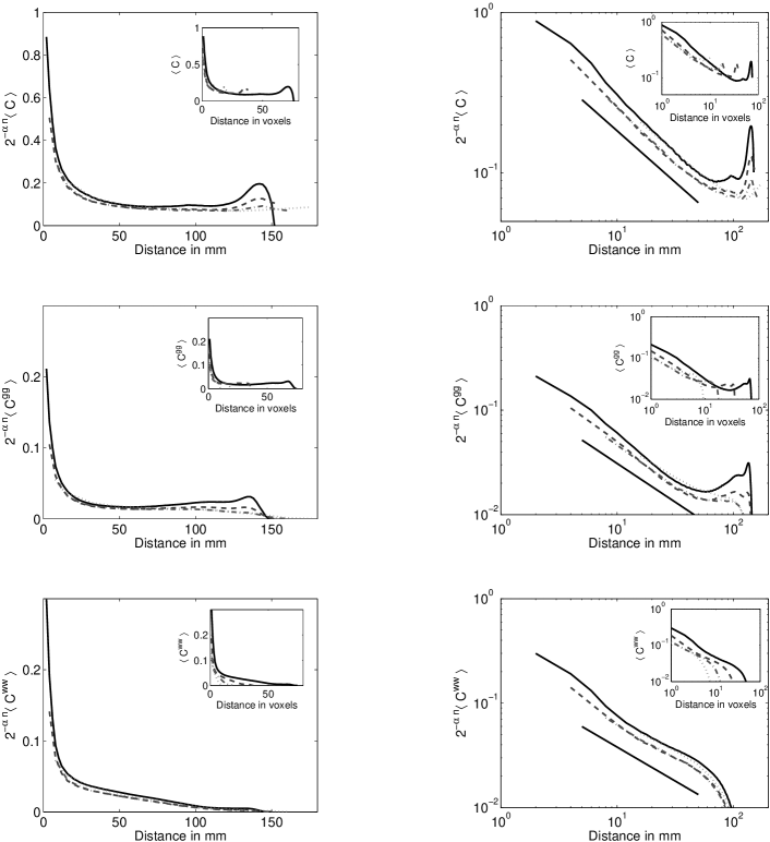
I Results

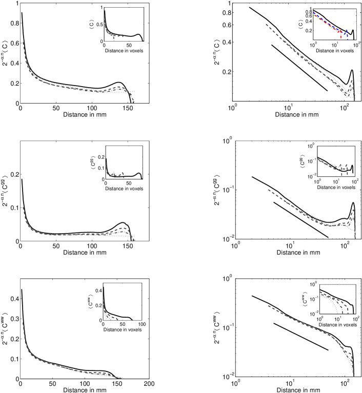
Spatial Self-similarity: Starting from the computation of the correlation matrix, the average correlation function for each separation $r$ can be estimated. To study the degree of self-similarity present in the correlation function, we perform a coarse-graining procedure and check for self-similarity via Eq. (7) as detailed in the section of Material and Methods. The result of this analysis for a single subject is shown in Fig. (1). The Supplementary Material (see below) contains the results for six additional subjects. In all cases, the data were binned into integer distance values to decrease the statistical fluctuations (especially at long distances) without having to average across several subjects. Two different regimes are observed in the correlation function. At short distances, we see a collapse of the different curves so Eq. (7) holds indicating that the system is self-similar. At longer distances, instead of the usual decay of the correlation function that is observed in physical models, there is a plateau, probably due to the brain bilateral symmetry, as seen previously across cortical bilaterally homologous regions by Salvador et al. salvador2 ; salvador , and then an increase in the correlations, probably due to surface effects.

After one coarse-graining step, the length of a side of a block-voxel is twice the size of a voxel, but then we need to renormalize the Euclidean distance in the coarse-grained system by a factor $2$ to recover distance in voxels. If the system under consideration was infinite, then $\langle C(r)\rangle$ would be defined for all $r$ irrespectively of the level of description and they would be identical, see Eq. (7). However, as the system we consider is finite, there exists a maximum distance $r_{m}$ in the original system. After one coarse-graining step, this maximal distance equal to $r_{m}/2$ and after $n$ coarse-graining steps, this maximum distance equals $r_{m}/2^{n}$, measured in units of voxels at the $n$th coarse-graining level. If Eq. (7) holds, then it means that the system behaves in the same manner at all scales, up to the maximum distance possible. Furthermore, it allows for a data-collapse of the correlation functions by first re the distance $r$ in voxel units to Euclidean distances, $r\mapsto r2^{n}a$ where $a$ is the voxel spacing in Euclidean distance (say mm) in the original data and then renormalizing the correlation functions by the factor $2^{-\alpha n}$, where $\alpha$ is a subject-dependent parameter. It is easy to check that if the correlation function depends on distance through a power law with exponent $\beta$, that is, $\langle C(r)\rangle\propto r^{-\beta}$, then the exponent $\alpha$ in the renormalizing factor of the correlation function must be equal to $\beta$. The relation $\alpha=\beta$ is fulfilled for this regime.

Scaling is only expected to apply in an intermediate regime where the sizes of the coarse-grained voxels are big compared with the smallest length scale cut-off in the data, that is, the voxel scale set by the scanner, and the largest distance covered by the data, that is, the size of the brain. This is indeed observed in Fig. (1) where the data collapse is best for the three curves corresponding to the bigger block voxels.

Figure 2: The average correlation function $\langle C\rangle$ vs the voxel distance after one step of coarse graining ($64\times 64\times 16$) for fMRI data (solid line) spatially randomized voxels (dashed-dotted line) and temporal randomized voxels (dotted line). Shown is also the average correlation function for phantom data (dashed line). Top panel in linear-linear, middle in linear-log and bottom in log-log axis, respectively. The correlation function for the fMRI data decays as a power law, while the correlation function for the phantom data decays exponentially fast. The correlation function for the spatially randomized data is constant while it is zero for the temporally randomized data.

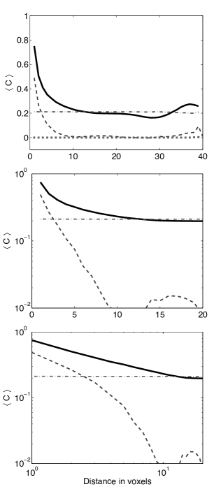
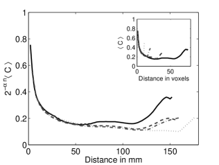
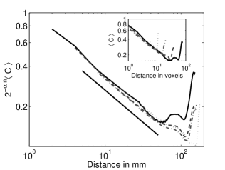
To verify that the shape of the average two-point correlation function is not due to artifacts in the data, we randomized the positions of the voxels or the time series, see Fig. (2). By randomizing the positions, we expect to find a constant profile for the correlations. In an infinite system or in a system where the correlation length is much smaller than the system’s size, this constant would be equal to zero, however, in the system we study strong long-range correlations are present, hence the constant is non-zero. By randomizing the time series of each voxel independently, we expect to destroy all correlation among voxels and thus expect close to zero average correlation for all distances. Furthermore, we also scanned a phantom to test our finding against artifact coming from the scanner. The phantom data shows an exponential decay and no long range correlation, except a peak at the longest distance that is also observed in brain data, confirming that it is a surface effect.

Pondering the Correlation Function with the Voxels’ Grey and White Matter Content: When analyzing fMRI data, the focus is, unlike our approach, generally on grey matter voxels. Due to the large millimeter size of the voxels, the discrimination between grey and white matter voxels is based on a high resolution anatomical scan that gives the content of grey matter, white matter and CSF for each voxels. A voxel is said to belong to grey/white matter if its content in the latter exceeds a threshold that has to be fixed, the others are dismissed. This procedure has the drawback that information is lost in the process, because the grey matter signal in dismissed voxels is lost.

Pure grey and white matter voxels are rare, but from a high resolution scan, we know the content of grey and white matter of each voxel. Hence, we can weight the correlations between two voxel according to their relative content of grey and white matter with the following normalization: $1=w^{g}+w^{w}+w^{CSF}$. We have performed the same analysis as we did above. Using all voxels weighted with their contents of grey and white matter, respectively, we calculated the average correlation functions

$$\langle C_{i,j}^{gg}\rangle=w_{i}^{g}w_{j}^{g}\langle C_{i,j}\rangle\quad\mbox{or}\quad\langle C_{i,j}^{\text{ww}}\rangle=w_{i}^{w}w_{j}^{w}\langle C_{i,j}\rangle.$$ (1)

Figure 3: The renormalized average correlation function $2^{-\alpha n}\langle C^{gg}\rangle$ of signal weighted with the content of grey matter vs real distance (inset: $\langle C^{gg}\rangle$ vs voxel distance) for the four levels of description for one subject. Full line: $128\times 128\times 31$ ($n=0$), dashed line: $64\times 64\times 16$ ($n=1$), dashed-dotted line: $32\times 32\times 8$ ($n=2$) and dotted line: $16\times 16\times 4$ ($n=3$). Top panel linear-linear and bottom panel log-log axis, respectively. Full straight line is a guide to the eye for a power law of exponent $\beta=0.60\pm 0.2$. Parameter $\alpha=0.35$.

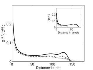
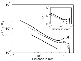
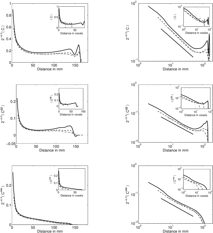
The correlation of grey matter is shown in Fig. 3 and the correlation of white matter is shown in Fig. 4. The bump at the end of the distribution survives only in the grey matter, which is to be expected, since it is probably due to a surface effect. White matter correlations die off smoothly before the surface of the brain is reached, which was expected since white matter is supposed to be enclosed in grey matter.

Figure 4: The renormalized average correlation function $2^{-\alpha n}\langle C^{\text{ww}}\rangle$ of signal weighted with the content of white matter vs real distance (inset: $\langle C^{\text{ww}}\rangle$ vs voxel distance) for the four levels of description for one subject. Full line: $128\times 128\times 31$ ($n=0$), dashed line: $64\times 64\times 16$ ($n=1$), dashed-dotted line: $32\times 32\times 8$ ($n=2$) and dotted line: $16\times 16\times 4$ ($n=3$). Top panel in linear-linear and bottom in log-log axis, respectively. Full straight line is a guide to the eye for a power law of exponent $\beta=0.61\pm 0.2$. Parameter $\alpha=0.20$.

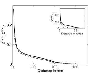
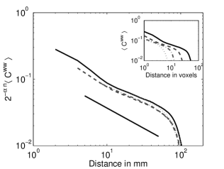
The fact that the exponents $\alpha\neq\beta$ in both Figs. 3 and 4 is related to the deviation from power-law behavior of the correlation functions of the grey and white matter. The scaling collapse is better for the correlation function when all voxels are included (see Fig. 1) than for the grey matter and white matter correlation functions displayed in Figs. 3 and 4. It is remarkable that only when the entire fMRI BOLD signal (all voxels without thresholding) is included in the correlation matrix we do obtain a good quality data collapse consistent with self-similarity. In general, we associate the essential dynamics and processing of the brain with grey matter, so our findings indicate that the separation of the fMRI BOLD signal using the weights $w^{g}$ and $w^{w}$ is more subtle than expected.

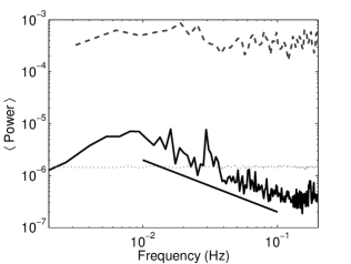
Temporal Self-similarity: To complement the spatial correlation analysis, we present the average power spectra of the fMRI time series. Temporal auto-correlations and power spectra have been studied by use of fMRI for a while. A comprehensive review is given in Woolrich-2001 and the use of these as a diagnostic tool was discussed in Bullmore-2005 . To obtain the spectra, we computed the spectrum of each voxel individually and normalized its integral to $1$. This corresponds to analyzing the Fourier transform of the auto-correlation function. We note that the term “power spectrum” is often used to denote the Fourier transform of the auto-covariance function. However, it is better to operate with the normalized correlation function to avoid signals with more power to totally dominate the average power spectra. Although the frequency range we can explore is rather small, the power spectrum has a reasonable $1/f$ dependence, thus showing criticality in time as well as in space, see Fig. (5). To check against potential artifacts of the measurement, we calculated the power spectra of phantom data and surrogate data, constructed by randomizing the brain fMRI time series. In both cases, we obtain a flat spectra as shown in Fig. (5) rejecting the possibility that the spectral features arise from scanning artifacts. The peak at $0.03\mbox{Hz}$ superimposed on the $1/f$ slope corresponds to the low-frequency fluctuations dynamics described already for the so-called brain resting-state networks beckmann2005 .

Figure 5: Average power spectrum for the fMRI time series (solid line), the phantom time series (dashed line) and the randomized time series (dotted line). Full straight line is a guide to the eye for a $1/f$ spectrum.

II Summary and Discussion

These results are the first direct demonstration of spatial and temporal self-similarity of the brain resting state dynamics. Although several reports already hinted about the possibility that at large-scale the brain may be operating in such state, previous measures have been indirect and/or model dependent. In contrast, in the present work scale invariance in space and time is determined from the entire data set without discarding any voxels and using the same renormalization techniques championed in the study of critical phenomena in physical systems and models.

It is interesting to relate our finding of scale invariance with the spatial and temporal localized functional activity extracted from fMRI data by Independent Component Analysis (ICA) methods. By construction, ICA emphasize the identification of strongly independent components and “filtering” out less important contributions to the total BOLD signal. Recent studies have investigated the growing complexity of the spatial structures extracted by ICA as the total numbers of components is allowed to increase Beckmann-2009 ; Kiviniemi-2009 . The additional structure obtained this way is indeed consistent with the self-similar character we have identified in the correlation function of the BOLD signal.

It should be mentioned that the distribution of BOLD fMRI spatiotemporal correlations was found already to be altered in certain chronic diseases baliki which together with the present result seem to suggest that scale invariance could be an important objective marker of brain well-being both in health and disease.

From a dynamical systems perspective, the uncovered self-similarity implies that the brain dynamics is permanently at an intermediate state between two extremes, one that is strongly correlated across large distances, producing transient highly integrated cortex states and the other in which only nearby clusters are acting in sync. This scenario, of long range correlations in space and time, is only conceivable in dynamical systems at criticality and could be the manner in which the cortex can manage to produce an arbitrarily large repertoire of interaction patterns among arbitrarily distant cortical sites.

III Materials and Methods

Image Acquisition: A 3T Philips MRI scanner was used to acquire T${}_{2}^{*}$-weighted echo-planer images (EPI) in $128\times 128\times 31$ voxels of dimension $2.5\times 2.5\times 5.0\,\mbox{mm}^{3}$ using a repetition time of $2000\,\mbox{ms}$, echo time of $60\,\mbox{ms}$ and a flip angle $90^{\circ}$. An 8-channel array coil and SENSE factor $2$ were used as well as second-order shims. Finally, a $3$-dimensional mask was used to identify the content of white matter, gray matter and CSF.

Image Pre-processing: The brain data consist of fMRI data sets of seven young adults healthy subjects in the resting state. The subjects were instructed to lie still in the scanner with their eyes closed avoiding falling asleep. A total of $305$ functional volumes of each subject were acquired from each session, the first five of which were discarded in order to remove the effect of T₁ equilibration. Image pre-processing was performed using the University of Oxford’s FMRIB software library (FSL) involving realigning to account for movement using FMRIB’s Linear Image Registration Tool (MCFLIRT) Jenkinson-2002 , high-pass temporal filtering using FEAT to remove low frequency artifacts and a high pass filter cutoff preset to $100\,\mbox{s}$.

Coarse Graining of the Signal: Coarse graining is a well established technique to describe system’s changes at different levels of spatial or temporal observation. This allows one to investigate to what extent the spatial or temporal structures of a given phenomena exhibits scale invariance, see for example Ref. Binney-1992 . A self-similar or scale invariance object, for instance a cauliflower, looks like itself at all scales. Each little bouquet of the cauliflower looks a miniature version of the entire cauliflower. Hence, a short length scale study of the cauliflower, in which one probes the substructure of an individual bouquet, will provide the same information as the study at a large length scale where one observe the cauliflower as a composition of bouquets.

In general, the approach to probe the behavior at different length scales consists in replacing the signal at a given point by a spatial average over a region of a given spatial extend about this point (see Fig. 6). In the case of an fMRI signal, the procedure consists in aggregating $2\times 2\times 2=8$ adjacent voxels to create a block-voxel ${\cal B}^{\prime}$ whose BOLD intensity at time $t$, $v_{{\cal B}^{\prime}}(t)$, is the average intensity of the BOLD intensities at time $t$, $v_{\cal B}(t)$ in its constituting voxels ${\cal B}\in{\cal B}^{\prime}$, that is,

$$v_{{\cal B}^{\prime}}(t)=\frac{1}{8}\sum_{{\cal B}\in{{\cal B}^{\prime}}}v_{\cal B}(t),$$ (2)

see Fig. 6 for an illustration.

Figure 6: (Left) Example of coarse graining in 2 dimensions where there are 4 boxes ${\cal B}$ within a block-box ${\cal B^{\prime}}$. (Right) The four dashed-colored signals from the four original boxes ${\cal B}$ are averaged to produce the solid-black coarse-grained signal of ${\cal B^{\prime}}$.

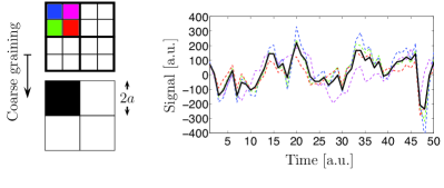
Computing Eq. 2 for all times $t=1,2,\ldots,300$ gives the time series for the BOLD signal in the block-voxels $\left\{v_{{\cal B}^{\prime}}(t)\right\}$. We now repeat the coarse-graining procedure on the time series for the BOLD signal in the block-voxels $\left\{v_{{\cal B}^{\prime}}(t)\right\}$ to produce a time series for the BOLD signal in the block-voxels $\left\{v_{\cal B^{\prime\prime}}(t)\right\}$ and so on. For the spatial resolution of our fMRI data, the coarse-graining procedure applied three times yield voxels ${\cal B}(128\!\times\!128\!\times\!31)\mapsto{\cal B^{\prime}}(64\!\times\!64\!\times\!16)\mapsto{\cal B^{\prime\prime}}(32\!\times\!32\!\times\!8)\mapsto{\cal B^{\prime\prime\prime}}(16\!\times\!16\!\times\!4)$ with associated signals $v_{\cal B}(t)\mapsto v_{\cal B^{\prime}}(t)\mapsto v_{\cal B^{\prime\prime}}(t)\mapsto v_{\cal B^{\prime\prime\prime}}(t)$. In the first coarse-graining step, the ultimate plane of voxels at the $31^{th}$ slice is coarse grained only along the $x-y$ plane. Averages has been calculated over active voxels only to prevent the inclusion of non-active voxels at the boundaries.

Next in our analysis, we consider the time series of each (block) voxel as a realization of a random variable and compute the time correlation matrix at the four levels of coarse graining. This matrix is obtained by computing the correlation between all pairs of (block) voxels ${\cal B}_{i}$ at position $\mathbf{r}_{i}$ and ${\cal B}_{j}$ at position $\mathbf{r}_{j}$:

$$C_{\cal B}\left(v_{{\cal B}_{i}},v_{{\cal B}_{j}}\right)=\frac{\frac{1}{T}\sum\limits_{t=1}^{T}v_{{\cal B}_{i}}(t)v_{{\cal B}_{j}}(t)-\hat{\mu}_{{\cal B}_{i}}\hat{\mu}_{{\cal B}_{j}}}{\hat{\sigma}_{{\cal B}_{i}}\hat{\sigma}_{{\cal B}_{j}}},$$ (3)

where $\hat{\mu}_{{\cal B}_{i}}=\frac{1}{T}\sum_{t=1}^{T}v_{{\cal B}_{i}}(t)$ is the temporal average value of (block) voxel’s ${\cal B}_{i}$ BOLD signal, and $\hat{\sigma}_{{\cal B}_{i}}=\sqrt{\frac{1}{T}\sum_{t=1}^{T}v^{2}_{{\cal B}_{i}}(t)-\hat{\mu}^{2}_{{{\cal B}_{i}}}}$ is the standard deviation of the BOLD signal of (block) voxel ${\cal B}_{i}$ and $T=300$.

Scaling: From the correlation matrix, the correlation function at equal time $C_{\cal B}\left(v_{{\cal B}_{i}},v_{{\cal B}_{j}}\right)$ is calculated as a function of the position in space of the voxels. We then compute the correlation function $\langle C_{\cal B}(r)\rangle$ averaged over all voxels with $r=\left|\mathbf{r}_{i}-\mathbf{r}_{j}\right|$ measured in units of (block) voxels. This is done for each level of coarse graining to obtain $\langle C_{\cal B}(r)\rangle$, $\langle C_{\cal B^{\prime}}(r)\rangle$, $\langle C_{\cal B^{\prime\prime}}(r)\rangle$ and $\langle C_{\cal B^{\prime\prime\prime}}(r)\rangle$ and the indices ${\cal B},{\cal B^{\prime}},{\cal B^{\prime\prime}}$ and ${\cal B^{\prime\prime\prime}}$ indicate the level of coarse graining

Let us discuss what to expect concerning the relation of the correlation function calculated at one coarse-graining level, say $\langle C_{\cal B}(r)\rangle$, compared to the one at the next level, $\langle C_{\cal B^{\prime}}(r)\rangle$. To clarify the effect of coarse graining, we relate the correlation function at this level of coarse graining to the covariance function at the previous level. For a homogeneous system, the covariance function is given by

$$\mbox{Cov}_{\cal B}(r)=\langle v_{\cal B}(0)v_{\cal B}(r)\rangle-\langle v_{\cal B}(0)\rangle\langle v_{\cal B}(0)\rangle,$$ (4)

where ${\langle\cdot\rangle}$ denotes spatial and temporal average. We consider, like in Eq. (2), the coarse graining over a block-voxel ${\cal B^{\prime}}$ centered at ${\bf r}$:

$$v_{\cal B^{\prime}}({\bf r})=\frac{1}{|{\cal B}|}\sum_{{\bf r+a}\in{\cal B^{\prime}}}v_{\cal B}({\bf r+a}),$$ (5)

where the block-voxel ${\cal B^{\prime}}$ contains $|{\cal B}|$ voxels. We then have

$$\langle C_{\cal B^{\prime}}(r)\rangle=\frac{\sum_{{\bf a}_{1},{\bf a}_{2}}\mbox{Cov}_{\cal B}({\bf r}+{\bf a}_{2}-{\bf a}_{1})}{\sum_{{\bf a}_{1},{\bf a}_{2}}\mbox{Cov}_{\cal B}({\bf a}_{2}-{\bf a}_{1})}.$$ (6)

For a scale invariant (self-similar) system of infinite size, $\langle C_{\cal B^{\prime}}(r)\rangle$ will remain invariant if distance $r$ is measured in units of coarse-graining boxes, that is,

$$\langle C_{\cal B}(r)\rangle=\langle C_{\cal B^{\prime}}(r)\rangle=\langle C_{\cal B^{\prime\prime}}(r)\rangle=\langle C_{\cal B^{\prime\prime\prime}}(r)\rangle.$$ (7)

Note that $r$ is the distance expressed in the voxel unit corresponding to the given level of coarse graining.

Figure 7: Main: The average correlation function $\langle C\rangle$ vs the block distance for three coarse-graining levels of an hypothetical object with a power-law form of the correlation function. The graphs collapse in voxel distance. Inset: Results from an hypothetical object having an exponential form of the correlation function where the curves do not collapse in block distance.

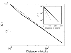
The simplest case of scale invariance corresponds to a power-law behavior of $\langle C(r)\rangle$. Figure 7 illustrates the different behavior under rescaling of two 3-dimensional artificial systems, where we imposed the correlation to have either a power-law or an exponential behavior:

$$\langle C(r)\rangle =\frac{1}{1+r},$$ (8a)

$$\langle C(r)\rangle =\exp(-r/5).$$ (8b)

Note that only the correlations having a power-law form do collapse in block unit.

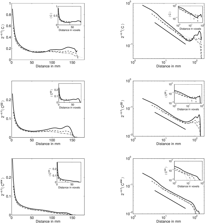
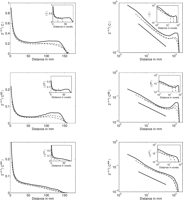
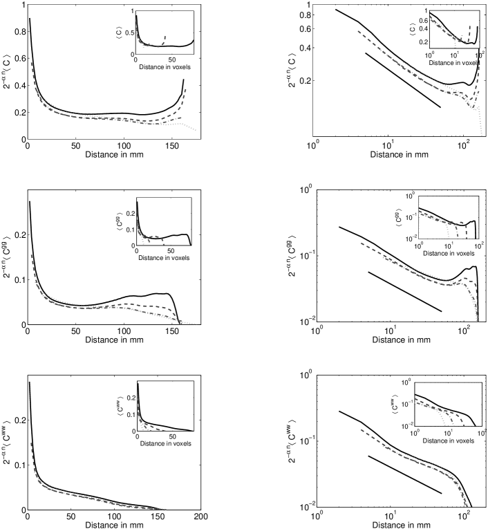
Supplementary information

The three average correlations $\langle C\rangle$, $\langle C^{gg}\rangle$ and $\langle C^{ww}\rangle$ at four levels of description for six additional subjects are consistent with the those presented in the main text. In general we find that the equality $\alpha=\beta$ is more accurately satisfied when only the three most coarse-grained data sets are included in the data collapse. Full line: $128\times 128\times 31$ ($n=0$), dashed line: $64\times 64\times 16$ ($n=1$), dashed-dotted line: $32\times 32\times 8$ ($n=2$) and dotted line: $16\times 16\times 4$ ($n=3$). Full straight line are guides to the eye for a power law with exponent $\beta$.

Figure S1: The renormalized average correlation functions $2^{-\alpha n}\langle C\rangle$ vs real distance (inset: $\langle C\rangle$ vs voxel distance). Left panel linear-linear and right panel log-log axis, respectively. Top panel $2^{-\alpha n}\langle C\rangle$ with $\beta=0.64\pm 0.2$ and $\alpha=0.51$, middle panel $2^{-\alpha n}\langle C^{gg}\rangle$ with $\beta=0.74\pm 0.2$ and $\alpha=0.50$ and bottom panel $2^{-\alpha n}\langle C^{ww}\rangle$ with $\beta=0.65\pm 0.2$ and $\alpha=0.40$, respectively.

Figure S2: The renormalized average correlation functions $2^{-\alpha n}\langle C\rangle$ vs real distance (inset: $\langle C\rangle$ vs voxel distance). Left panel linear-linear and right panel log-log axis, respectively. Top panel $2^{-\alpha n}\langle C\rangle$ with $\beta=0.51\pm 0.2$ and $\alpha=0.42$, middle panel $2^{-\alpha n}\langle C^{gg}\rangle$ with $\beta=0.62\pm 0.2$ and $\alpha=0.37$ and bottom panel $2^{-\alpha n}\langle C^{ww}\rangle$ with $\beta=0.65\pm 0.2$ and $\alpha=0.31$, respectively.

Figure S3: The renormalized average correlation functions $2^{-\alpha n}\langle C\rangle$ vs real distance (inset: $\langle C\rangle$ vs voxel distance). Left panel linear-linear and right panel log-log axis, respectively. Top panel $2^{-\alpha n}\langle C\rangle$ with $\beta=0.46\pm 0.2$ and $\alpha=0.37$, middle panel $2^{-\alpha n}\langle C^{gg}\rangle$ with $\beta=0.55\pm 0.2$ and $\alpha=0.40$ and bottom panel $2^{-\alpha n}\langle C^{ww}\rangle$ with $\beta=0.52\pm 0.2$ and $\alpha=0.25$, respectively.

Figure S4: The renormalized average correlation functions $2^{-\alpha n}\langle C\rangle$ vs real distance (inset: $\langle C\rangle$ vs voxel distance). Left panel linear-linear and right panel log-log axis, respectively. Top panel $2^{-\alpha n}\langle C\rangle$ with $\beta=0.50\pm 0.2$ and $\alpha=0.41$, middle panel $2^{-\alpha n}\langle C^{gg}\rangle$ with $\beta=0.60\pm 0.2$ and $\alpha=0.37$ and bottom panel $2^{-\alpha n}\langle C^{ww}\rangle$ with $\beta=0.57\pm 0.2$ and $\alpha=0.30$, respectively.

Figure S5: The renormalized average correlation functions $2^{-\alpha n}\langle C\rangle$ vs real distance (inset: $\langle C\rangle$ vs voxel distance). Left panel linear-linear and right panel log-log axis, respectively. Top panel $2^{-\alpha n}\langle C\rangle$ with $\beta=0.47\pm 0.2$ and $\alpha=0.34$, middle panel $2^{-\alpha n}\langle C^{gg}\rangle$ with $\beta=0.72\pm 0.2$ and $\alpha=0.58$ and bottom panel $2^{-\alpha n}\langle C^{ww}\rangle$ with $\beta=0.55\pm 0.2$ and $\alpha=0.17$, respectively.

Figure S6: The renormalized average correlation functions $2^{-\alpha n}\langle C\rangle$ vs real distance (inset: $\langle C\rangle$ vs voxel distance). Left panel linear-linear and right panel log-log axis, respectively. Top panel $2^{-\alpha n}\langle C\rangle$ with $\beta=0.49\pm 0.2$ and $\alpha=0.39$, middle panel $2^{-\alpha n}\langle C^{gg}\rangle$ with $\beta=0.60\pm 0.2$ and $\alpha=0.36$ and bottom panel $2^{-\alpha n}\langle C^{ww}\rangle$ with $\beta=0.62\pm 0.2$ and $\alpha=0.29$, respectively.