Simple heuristics for the assembly line worker assignment and balancing problem

Abstract

We propose simple heuristics for the assembly line worker assignment and balancing problem. This problem typically occurs in assembly lines in sheltered work centers for the disabled. Different from the classical simple assembly line balancing problem, the task execution times vary according to the assigned worker. We develop a constructive heuristic framework based on task and worker priority rules defining the order in which the tasks and workers should be assigned to the workstations. We present a number of such rules and compare their performance across three possible uses: as a stand-alone method, as an initial solution generator for meta-heuristics, and as a decoder for a hybrid genetic algorithm. Our results show that the heuristics are fast, they obtain good results as a stand-alone method and are efficient when used as a initial solution generator or as a solution decoder within more elaborate approaches.

1 Introduction

In assembly lines, products are assembled by means of the successive execution of tasks in workstations. Each task has an execution time and precedence relationships with other tasks. The simple assembly line balancing problem (SALBP) concerns the decision of allocating tasks to the workstations while respecting the partial ordering of the tasks. Let $c$ be the cycle time of the line, i.e., the time spent at one of the workstations with the heaviest workload and $m$ be the number of workstations. The problem is known as SALBP-1 when the goal is to minimize $m$ given a maximum allowed $c$, SALBP-2 when the goal is to minimize $c$ given a fixed $m$, SALBP-E when one wants to minimize $m\cdot c$ and SALBP-F when the goal is to decide whether a feasible solution does exist for given $m$ and $c$. For more details on SALBP and many of its variants, we refer the reader to Baybars (1986), Scholl (1999) Scholl and Becker (2006), Boysen et al (2007), and Boysen et al (2008).

The assembly line worker assignment and balancing problem (ALWABP) is an extension of the SALBP in which task execution times are worker-dependent. This problem typically occurs when balancing assembly lines with disabled workers, because a given worker might be efficient on a certain subset of the tasks while being inefficient on (or even unable of executing) other tasks. Analagous to the SALBP, variants ALWABP-1, -2, -E and -F can also be defined.

The ALWABP has been introduced in the literature by Miralles et al (2007) by means of a case study in an assembly line of a Spanish sheltered work center for the disabled where a fixed number of workers should be present in an assembly line whose production rate should be maximized (ALWABP-2). The same authors have later developed a branch-and-bound algorithm for the problem, enabling the solution of small-sized instances (Miralles et al, 2008). Because of the problem complexity and the need to solve larger instances, the literature has since then shifted its efforts to heuristic methods. Chaves et al (2009) have proposed an elaborate clustering search algorithm that obtained good solutions in reasonable computation times for instances of up to 19 workers. Their algorithm relies on a clustering procedure to group, analyze and improve the solutions generated by a meta-heuristic approach. In the search of a simpler method, Moreira and Costa (2009) have proposed a minimalist tabu search algorithm based on the use of objective function penalties associated to infeasible solutions to improve the algorithms ability to effectively explore the search space. More recently, Blum and Miralles (2011) have developed a beam search algorithm which has been successful in improving the best known solutions obtained in the previously mentioned studies.

In this study, we develop and test constructive heuristics for the ALWABP-2. The heuristics generalize station-oriented assignment procedures for the SALBP and apply them in search procedures for finding the minimum cycle time (Scholl and Voß, 1996). Station-oriented assignment procedures sequentially process the stations and assign tasks to the current station in an order defined by a priority rule until it is maximally loaded. The extension of such procedures to the ALWABP-2 is not immediate, since the priority rules are often based on the task execution times, a parameter that in the ALWABP depends on the worker assigned to each workstation which is itself an optimization decision.

The idea of our method is to use task and worker priority rules to define which worker and which set of tasks will be assigned to each workstation. We define 16 task priority rules and three worker priority rules. The heuristic efficiency is compared by means of computational tests to evaluate its performance both as a stand-alone method as well as its ability to improve the convergence of more sophisticated methods such as the aforementioned clustering search and tabu search algorithms (Chaves et al, 2009; Moreira and Costa, 2009). Moreover, the proposed heuristic is also used as a solution decoder within a hybrid genetic algorithm that optimizes explicit priorities for each task-worker pair.

The remainder of this paper is organized as follows. Next, we present a formal definition of the ALWABP and a mixed-integer linear model for the problem. Then, the proposed heuristic is detailed in Section 3 and its use within a hybrid genetic algorithm is described in Section 4. A computational study is presented in Section 5 and this paper ends with some conclusions in Section 6.

2 Formal problem definition and mathematical model

In this section we present a formal definition of the ALWABP-2. As mentioned before, we denote by $c$ the cycle time and by $m$ the number of workstations. Let $N$ be the set of tasks to be allocated. The precedence constraints are given by a directed acyclic graph $G=(N,E)$ over this set of tasks, where each edge $ij\in E$ indicates that task $i$ is an immediate predecessor of task $j$. We also define an extended version of the precedence graph known as the transitive closure of $G$, $G^{*}=(N,E^{*})$, in which $ij\in E^{*}$ if there is a path from $i$ to $j$ in $G$. In addition we will use the following notation in the remainder of this paper:

$S$	set of workstations;
$W$	set of workers, $|W|=|S|$;
$t_{i}\in\mathbb{N}$	time of task $i$ (SALBP);
$t_{wi}\in\mathbb{N}\cup\{\infty\}$	time of task $i$ when executed by worker $w$ (ALWABP);
$I_{w}=\{i\in N\mid t_{wi}=\infty\}$	set of tasks infeasible for worker $w$;
$P_{i}=\{j\mid ji\in E\}$	set of immediate predecessors of task $i$;
$P^{*}_{i}=\{j\mid ji\in E^{*}\}$	set of all predecessors of task $i$;
$F_{i}=\{j\mid ij\in E\}$	set of immediate successors of task $i$;
$F^{*}_{i}=\{j\mid ij\in E^{*}\}$	set of all successors of task $i$.

The goal of the problem is, given a fixed number of workstations, $\overline{m}$, to find an assignment of tasks and workers to the workstations minimizing $c$ and such that each task $i\in N$ is assigned to a single station $s\in S$ and the precedence relationships are respected, i.e., a task $i\in P_{j}$ can only be assigned to the same workstation to which task $j$ has been assigned or to workstations preceding it. We consider an equal number of workstations and workers and, therefore, each worker $w\in W$ must be assigned to a single station $s\in S$. Likewise, each workstation $s\in S$ must receive a single worker $w\in W$. Workers cannot be assigned independently from the task assignments, since the total load of a workstation depends both on the tasks and the worker assigned to it.

A mathematical model has been proposed by Miralles et al (2008). The authors define binary variables $x_{swi}$, equal to 1 only if task $i$ is assigned to worker $w$ at workstation $s$, and binary variables $y_{sw}$, equal to 1 only if worker $w$ is assigned to workstation $s$. The model can be written as below:

Minimize $$c$$ (1)

subject to $$\sum_{w\in W}\sum_{s\in S}x_{swi}=1 \forall i\in N,$$ (2)

$$\sum_{s\in S}y_{sw}=1 \forall w\in W,$$ (3)

$$\sum_{w\in W}y_{sw}=1 \forall s\in S,$$ (4)

$$\sum_{w\in W}\sum_{s\in S}sx_{swi}\leq\sum_{w\in W}\sum_{s\in S}sx_{swj} \forall i,j\in N|i\in P_{j},$$ (5)

$$\sum_{w\in W}\sum_{i\in N}t_{wi}x_{swi}\leq c \forall s\in S,$$ (6)

$$\sum_{i\in N}x_{swi}\leq|N|y_{sw} \forall w\in W,\forall s\in S,$$ (7)

$$x_{swi}=0 \forall w\in W,\forall s\in S,\forall i\in I_{w},$$ (8)

$$y_{sw}\in\{0,1\} \forall s\in S,\forall w\in W,$$ (9)

$$x_{swi}\in\{0,1\} \forall s\in S,\forall w\in W,\forall i\in N.$$ (10)

Model (1)–(10) focuses on minimizing the cycle time for a given number of workstations. Constraints (2) guarantee that each task is executed, and that it is done by a single worker, at a single workstation. Constraints (3) and (4) establish a bijection between workers and workstations at a feasible solution, i.e., every worker is assigned to a single workstation and vice versa. Constraints (5) define the precedence relations. Constraints (6) establish that the cycle time is the sum of the execution times of the tasks at the most charged workstation, by forcing $c$ to be larger than or equal to the load assigned to each station. Finally, constraints (7) indicate that a task can only be assigned to a worker in a given workstation if that worker is also assigned to the workstation.

The difficulty in solving this model has been reported in the literature (Miralles et al, 2008) and motivates the search for efficient heuristic methods like the constructive heuristics presented in the following section.

3 Constructive heuristic methods

In this section we propose a constructive heuristic framework for the ALWABP which is based on heuristics for the SALBP presented by Scholl and Voß (1996). In order to simplify the presentation, we describe the original heuristic in Section 3.1 and present the new developments in Section 3.2.

3.1 Constructive heuristics for the SALBP

The strategy used by Scholl and Voß (1996) to solve the SALBP-2 relies on solving instances of SALBP-1 for different cycle times. A given cycle time $c$ can be considered an upper bound for the SALBP-2 if the solution of the SALBP-1 needs, at most, the desired number of workstations $\overline{m}$.

The solution of the SALBP-1 instances can rely upon exact or approximate methods. Since the SALBP-1 is also an NP-hard problem, heuristic methods are often used. These methods are usually based on priority rules that order the tasks according to a given criterion and assign them to the workstations accordingly. An important notion is that of an available task, which is an unassigned task whose predecessors have already been assigned. Let $\overline{c}$ be the desired cycle time and $t(S_{k})$ the station time of workstation $k$. A station-oriented procedure to solve the SALBP-1 can be easily described in three steps:

Algorithm 1 Station-oriented assignment procedure for the SALBP-1

0:  maximum cycle time $\overline{c}$

1:  Start at an empty workstation $k=0$, $t(S_{k})=0$. Set the unassigned tasks to $U=N$.

2:  Assign to the current workstation the available task $i$ with highest priority such that $t_{i}+t(S_{k})\leq\overline{c}$ and set $U=U\backslash\{i\}$.

3:  If no more tasks are available, return $k$ (end). Otherwise, if there are available tasks, but none can be assigned to the current workstation $k$, set $k=k+1$, $t(S_{k})=0$. Go to step 2.

Scholl and Voß (1996) mention the following selection of successful priority rules, defining different orders with which the tasks should be considered for assignment:

1. MaxF: descending number of followers, $|F^{*}_{i}|$;

2. MaxIF: descending number of immediate followers, $|F_{i}|$;

3. MaxTime: descending task times, $t_{i}$;

4. MaxPW: descending positional weights, $pw_{i}=t_{i}+\sum_{h\in F^{*}_{i}}t_{h}$;

5. MaxTimeL: descending task time divided by latest station, $t_{i}/L_{i}$;

6. MaxTimeSlack: descending task time divided by slack, $t_{i}/s_{i}$

where $E_{i}$ and $L_{i}$ are the earliest and latest workstations (defined in Section 3.2.3) to which a task can be assigned and still obey the precedence constraints and the desired cycle time $\overline{c}$, and where $s_{i}=L_{i}-E_{i}$ is the slack of task $i$ (Scholl, 1999).

With these priority rules, an algorithm for the SALBP-2 can be developed by searching for the smallest feasible $\overline{c}$. Scholl and Voß (1996) mention several search procedures such as the lower bound method and binary search. In this paper, we use the lower bound method in all our heuristics, since it finds the smallest possible $\overline{c}$ for a given SALBP-1 heuristic.

3.2 Extension to the ALWABP

The extension of the SALBP priority rules to the ALWABP faces two main difficulties. First, most of the priority rules rely on task execution times, which are not well defined for the case of the ALWABP since they depend on the designated worker. Second, there is no strategy to select the worker to be assigned to each workstation. In the following, we propose modifications to the original algorithm in order to cope with these two difficulties.

3.2.1 Task priority rules

From the six priority rules suggested by Scholl and Voß (1996), the first two can be used unchanged in ALWABP, because they do not depend on task execution times. Rules MaxTime and MaxPW do depend on task execution times but can still be adapted if one considers, for instance, minimum, maximum or averaged values of these times over all workers. In particular, for the original rule MaxTime based on task execution times, we considered ascending and descending orderings for each possibility. Finally, the last two rules depend on the earliest and latest stations to which a task can be assigned; we do decided to not apply these rules since the corresponding station bounds are rather weak for ALWABP.

The proposed adaptions lead to eleven rules for the ALWABP derived from existing rules for the SALBP. We further propose five new rules that try to reflect the structure of the ALWABP by using the original task execution times per worker. The idea is to prioritize tasks when workers that quickly execute these tasks are being considered. The full set of priority rules are listed and described in the following, where $\overline{w}_{i}\in\mathrm{\operatorname*{argmin}}_{w\in W}t_{wi}$ is some fastest worker in the execution of task $i$ and $t_{i}^{-}=\textrm{min}_{w\in W}t_{wi}$, $t_{i}^{+}=\textrm{max}_{w\in W}t_{wi}$, $\overline{t}_{i}=\sum_{w\in W}t_{wi}/|W|$ are the minimum, maximum and mean execution time of task $i$, respectively. If task $i$ is infeasible for worker $w$, i.e., $t_{wi}=\infty$, we set $t_{wi}=\overline{c}$ for the purposes of computing $t_{i}^{+}$ and $\overline{t}_{i}$, where $\overline{c}$ is cycle time under consideration (see Algorithm 2).

1. MaxF: descending number of followers, $|F^{*}_{i}|$;

2. MaxIF: descending number of immediate followers, $|F_{i}|$;

3. MaxTime^-: descending minimum task times, $t_{i}^{-}$;

4. MaxTime⁺: descending maximum task times, $t_{i}^{+}$;

5. Max$\overline{\textrm{Time}}$: descending average task times, $\overline{t}_{i}$;

6. MinTime^-: ascending minimum task time, $t_{i}^{-}$;

7. MinTime⁺: ascending maximum task time, $t_{i}^{+}$;

8. Min$\overline{\textrm{Time}}$: ascending average task time, $\overline{t}_{i}$;

9. MaxPW^-: descending minimum positional weights, $pw_{i}^{-}=t_{i}^{-}+\sum_{h\in F^{*}_{i}}t_{h}^{-}$;

10. MaxPW⁺: descending maximum positional weights, $pw_{i}^{+}=t_{i}^{+}+\sum_{h\in F^{*}_{i}}t_{h}^{+}$;

11. Max$\overline{\textrm{PW}}$: descending average positional weights, $\overline{pw_{i}}=\overline{t}_{i}+\sum_{h\in F^{*}_{i}}\overline{t}_{h}$;

12. MinD(w): ascending difference to best worker, $t_{wi}-t_{\overline{w}_{i}i}$;

13. MinR(w): ascending ratio to best worker, $t_{wi}/t_{\overline{w}_{i}i}$;

14. MaxFTime(w): descending number of followers per time, $|F_{i}|/t_{wi}$;

15. MaxIFTime(w): descending number of immediate followers per time, $|F^{*}_{i}|/t_{wi}$;

16. MinRank(w): ascending rank of worker’s execution time, $|\{w^{\prime}\in W\mid t_{w^{\prime}i}<t_{wi}\}|$.

Rules MinD(w) and MinR(w) prioritize tasks for which the current worker w is faster than other workers while MaxFTime(w) and MaxIFTime(w) balance two desired characteristics of a task: it should be executed quickly by the current worker $w$ and it should make the largest number of tasks available. For the current worker $w$, rule MinRank(w) gives preference to a task with a short execution time compared to other workers, but does not depend on concrete execution times. The other rules follow the original rationale.

3.2.2 Worker priority rules

Many of the task priority rules proposed above analyze the efficiency of a given worker for the task in comparison to the other workers. This suggests that Algorithm 1 needs to be modified to include a worker selection loop in which all possible workers are tested and, according to a worker selection criterion, one is chosen for the current workstation. This modification is reflected in Algorithm 2. We also add an outer while loop on cycle time tentative values, in order to present a self-contained algorithm for the ALWABP-2.

Algorithm 2 Station-oriented assignment procedure for the ALWABP-2

1:  $\overline{c}$ = lower bound on the cycle time.

2:  while solution not found do

3:     Start at an empty workstation $k=0$, $t(S_{k})=0$.

4:     Set the unassigned workers to $U_{w}=W$, set the unassigned tasks to $U=N$.

5:     for each worker $w$ in $U_{w}$ do

6:        Compute $T_{w}$, the set of tasks that would be assigned to worker $w$ according to the task priority rule used.

7:     end for

8:     Assign the worker $w$ with the highest priority and its tasks $T_{w}$ to the station $k$. $U_{w}=U_{w}\backslash\{w\}$, $U=U\backslash T_{w}$, $k=k+1$.

9:     if  $U_{w}\neq\emptyset$  then

10:        Go to step 4.

11:     else

12:        if $U=\emptyset$ then

13:           return  $\overline{c}$

14:        else

15:           $\overline{c}=\overline{c}+1$

16:        end if

17:     end if

18:  end while

Algorithm 2 tests, for each workstation, all unassigned workers. In step 6, the algorithm computes the tasks that can be assigned to the current station if the worker under consideration is also assigned to that station. Note that these tasks depend on the priority rule, on the worker and on the tentative cycle time being considered. In step 8, according to the selected tasks, it chooses the worker which will be assigned to the current workstation. Let $t_{i}^{-}(W)=\min_{w\in W}t_{wi}$ be the minimum execution time of task $i$ among workers $W$. We propose three worker selection rules:

• MaxTasks: descending number of assignable tasks, $|T_{w}|$;

• MinBWA: ascending best worker assignment cycle MinBWA($U\setminus T_{w}$,$U_{w}\setminus\{w\}$) (Algorithm 3).

• MinRLB: ascending restricted lower bound,

  $$\frac{\sum_{i\in U\backslash T_{w}}\;t_{i}^{-}(U_{w}\setminus\{w\})}{|U_{w}|-1}\mathrm{.}$$

Algorithm 3 Best worker assignment cycle (MinBWA)

1:  input: a set of tasks $T$ and workers $W$

2:  Set $t_{w}=0$ for all $w$ in $W$

3:  for each task $i$ in $T$ do

4:     Determine the set of workers executing $i$ fastest, $W^{\prime}:=\operatorname*{argmin}_{w\in W}t_{wi}$

5:     Select a worker $w^{\prime}\in W^{\prime}$ of minimum load $t_{w^{\prime}}=\min_{w\in W^{\prime}}t_{w}$

6:     $t_{w^{\prime}}=t_{w^{\prime}}+t_{w^{\prime}i}$

7:  end for

8:  return  the maximum cycle time $c=\max_{w\in W}t_{w}$

The first rule gives preference to the worker that was able to execute the largest number of tasks. The last two criteria compute estimates on the cycle time for the problem considering the yet unassigned workers and tasks, and give preference to the worker that reduces this estimate. They differ on the way the estimates are obtained. Rule MinBWA computes the cycle time that would be obtained if each remaining worker were assigned the tasks which he executes fastest (in case of ties, the task is attributed to the currently less charged worker). Rule MinRLB computes a lower bound for the cycle time on the remaining workstations by dividing the sum of the minimum execution times of the remaining tasks by the number of remaining workers.

Each of these three worker priority rules can be combined with one of the above $16$ task priority rules. Moreover, if one considers that the station-oriented assignment can be run in a forward (considering the original precedence graph) or backward (considering the reversed precedence graph) manner, a total of $96$ possible combinations are possible. The efficiency of these combinations is compared in Section 5.

3.2.3 Bounds on the minimum cycle time

In order to reduce the number of calls made to Algorithm 2 and, therefore, improve the efficiency of the method, one might investigate good lower bounds for the ALWABP-2. Valid lower bounds for the SALBP-2 can be used by substituting the task execution time in the original bound by the minimum task execution time over all workers $t_{i}^{-}$. With this strategy, we are able to use lower bounds LC1, LC2, and LC3 from Scholl and Becker (2006) in our search procedures. LC1 and LC2 are defined as

$$\mathrm{LC1} :=\max\biggl{\{}\max_{i\in N}t_{i}^{-},\biggl{\lceil}\sum_{i\in N}t_{i}^{-}/m\biggl{\rceil}\biggr{\}}$$

$$\mathrm{LC2} :=\max\biggl{\{}\sum_{0\leq i\leq k}t^{-}_{km+1-i}\mid 1\leq k\leq\bigl{\lfloor}(n-1)/m\bigr{\rfloor}\biggr{\}}\mathrm{.}$$

The bound LC3 is obtained by destructive improvement (Klein and Scholl, 1999) using bounds on the earliest station $E_{i}(c)$ and latest station $L_{i}(c)$ for each task $i$, and is defined as the smallest $c$ greater than or equal to an initial lower bound $\underline{c}$ such that $E_{i}(c)\leq L_{i}(c)$ for all tasks $i$. When using minimum task times, the station bounds are defined as

$$E_{i}(c) :=\biggl{\lceil}\biggl{(}\sum_{j\in P^{*}_{i}}t^{-}_{j}+t^{-}_{i}\biggr{)}/c\biggr{\rceil}$$

$$L_{i}(c) :=m+1-\biggl{\lceil}\biggl{(}t^{-}_{i}+\sum_{j\in F^{*}_{i}}t^{-}_{j}\biggr{)}/c\biggr{\rceil}\mathrm{.}$$

For a given cycle time $c$, these bounds can be improved by preprocessing the ALWABP-2 instance as follows. For tasks $i,k$ let $O(i,k)=(F_{i}^{*}\cap P_{k}^{*})\cup(F_{k}^{*}\cap P_{i}^{*})$ be the tasks that must be executed after $i$ and before $k$ or vice-versa, and let $R(i,k)=O(i,k)\cup\{i,k\}$. If some task $i$ can only be executed by a given worker $w$, then another task $k$ can be executed by the same worker $w$ only if the total execution time of all tasks between $i$ and $k$ does not exceed $c$, i.e., $\sum_{j\in R(i,k)}t_{wj}\leq c$. Otherwise, task $k$ is infeasible for worker $w$. In this latter case, a reduced instance for a cycle time $c$ can be obtained by setting the execution time $t_{wk}$ of all such tasks to $\infty$, making them infeasible for worker $w$.

As a fourth bound we use the linear relaxation of model (1)–(10). For SALBP-2 the linear relaxation of the ILP-model is known to be weak, but this bound proves to be useful for ALWABP-2, because the use of minimum execution times weakens the lower bounds LC1, LC2, and LC3. Since this bound is the most expensive computationally, it is used only in the genetic algorithm presented in the next section.

4 A hybrid genetic algorithm for ALWABP-2

In this section we propose a hybrid biased random-key genetic algorithm (HGA) based on the constructive heuristic of Section 3. Random-key genetic algorithms are particularly useful for sequencing problems, and have been proposed by Gonçalves and de Almeida (2004) for the SALBP-1 and, by Mendes et al (2009) for resource constrained project scheduling.

A genetic algorithm (Goldberg, 1989; Holland, 1975) is a population-based meta-heuristic. Each individual in the population has a chromosome which codifies a solution to a problem instance. A chromosome consists of a collection of genes each of which can take a value among several alleles. A population generates offspring by crossover between two individuals and mutation. The probability of an individual to participate in a crossover is proportional to its fitness, making it more likely that fitter individuals pass genetic material to the next generation. A selection rule determines which individuals from the current generation and the offspring form the next generation.

Bean (1994) introduced random-key genetic algorithms (RKGA). In a RKGA the chromosome is a vector in $\mathbb{R}^{n}$ (where $n$ is a problem-dependent parameter) and a decoder maps it to a feasible solution. For example, in problems of sequencing jobs, the order of the genes’ values defines a permutation of the jobs. The advantage of an RKGA is that the decoding process guarantees that each chromosome corresponds to a feasible solution and that the search can be done in a problem-independent way in the space $\mathbb{R}^{n}$.

The evolutionary dynamics of a RKGA is as follows. All $p$ individuals in the current population are sorted by their fitness value, and the best $p_{e}$ elite individuals are copied into the next generation. A RKGA replaces mutation by immigration of a small percentage $p_{r}$ of random individuals into the next generation. The remaining $p-p_{e}-p_{r}$ individuals are offspring. To generate offspring, two individuals are selected at random from the current population and are combined by uniform crossover. In uniform crossover, the offspring receives each allele independently with probability $q\geq 0.5$ from the first parent and probability $1-q$ from the second parent.

A biased random-key genetic algorithm differs from a RKGA in the way it selects parents for crossover. The first parent is drawn randomly from the elite set, and the second one randomly from the remaining individuals. In this way, the offspring inherits with a higher probability an allele from an elite parent. A hybrid genetic algorithm applies a local search method to its individuals to improve their fitness.

To construct a HGA for the ALWABP-2, we substitute the task priority rules presented in Section 3 by explicit priorities. Instead of using a rule to define a priority $\mathrm{pr}(w,i)$ for each worker $w$ and task $i$, the chromosome of an individual in the HGA is a matrix $p_{wi}$ of priorities in $[0,1]$. The fitness of an individual is the result of Algorithm 2 run with these priorities. Algorithm 2 uses the bounds described in Section 3.2.3, including the linear relaxation lower bound, when searching for a feasible cycle time. To find a feasible solution, it tries to allocate all tasks in a forward as well as a backward manner.

After decoding, a local search is applied to improve the solution. The local search uses two types of well-known moves (Scholl and Becker, 2006): a shift of a task from one station to another, and a swap of two tasks between different stations. We allow also a sequence of two shifts, where the first one does not improve the solution. A third move type applied in the local search is a swap of two workers between two stations. All moves are applied only when they produce a feasible solution and are able to reduce the number of stations with load equal to the cycle time.

The fitness of an individual is a pair $(c,l)$, where $c$ is the smallest cycle time found after local search, and $l$ is the normalized total station time, i.e., the sum of all task execution times divided by $mc$. Fitness is ordered lexicographically. The second component allows the HGA to reduce, for a constant cycle time $c$, the station times of a solution.

The initial population is seeded with individuals whose priorities are set according to the $16$ proposed task priority rules. If the population size is less than $16$ we select the $p$ best individuals. For populations larger than $16$, the remaining individuals of the population are initialized randomly. The pseudo-code for the HGA is shown in Algorithm 4.

Algorithm 4 HGA for the ALWABP-2

1:  input: population sizes $p$, $p_{e}$, $p_{r}$, crossover probability $q$;

2:  {We denote by $f(i)$ the fitness of individual $i$}

3:  $P:=\{(i_{1},f(i_{1})),\ldots,(i_{16},f(i_{16}))\}$ where $i_{k}\in[0,1]^{|W|\times|N|}$, $1\leq k\leq 16$ is set using task priority rule $k$;

4:  $P:=P\cup\{(i_{17},f(i_{17})),\ldots,(i_{p},f(i_{p}))\}$ where each $i_{k}$, $17\leq k\leq p$ is a random matrix in $[0,1]^{|W|\times|N|}$;

5:  sort $P$ by increasing cycle times $f(i_{k})$ and keep the $p$ best individuals;

6:  while stopping criterion is not satisfied do

7:     $P^{\prime}:=\{(i_{1},f(i_{1})),\ldots,(i_{p_{e}},f(i_{p_{e}})\}$; { elite passes to the next generation }

8:     for $k=1,\ldots,p-p_{e}-p_{r}$ do

9:        select a random individual $i$ from $\{i_{1},\ldots,i_{p_{e}}\}$;

10:        select a random individual $j$ from $\{i_{p_{e}+1},\ldots,i_{p}\}$;

11:        $o:=\mathrm{crossover}(i,j,q)$;

12:        $\mathrm{localsearch}(o)$;

13:        $P^{\prime}:=P^{\prime}\cup\{(o,f(o))\}$;

14:     end for

15:     for $k=1,\ldots,p_{r}$ do

16:        $P^{\prime}:=P^{\prime}\cup\{(i,f(i))\}$ where $i$ is a random matrix in $[0,1]^{|W|\times|N|}$;

17:     end for

18:     $P:=P^{\prime}$;

19:     sort $P$ by increasing cycle times $f(i_{k})$;

20:  end while

21:  return  best individual $i_{1}$;

5 Computational study

In this section, we present a computational study of the proposed lower bounds, the constructive heuristics, and the hybrid genetic algorithm. In all experiments, we have used the instances available in the literature (Chaves et al, 2007). They are grouped in four families: Roszieg, Heskia, Wee-Mag and Tonge, each one containing $80$ instances. The instances were generated from the corresponding SALBP instances such that they contain $10$ instances for each combination of five experimental factors at a low and a high level. The factors are the number of tasks, the number of workers, the order strength, the variability of the task execution time, and the number of infeasible task-worker pairs. For instances with low variability, the task execution times are drawn uniformly from the interval $[1,t_{i}]$, where $t_{i}$ is the task execution time as defined by the SALBP instance. When the variability is high, this interval was $[1,3t_{i}]$. The number of infeasible task-worker pairs is $10\%$ and $20\%$ on the low and the high level, respectively. The main characteristics for each group of instances (number of tasks, number of workers and the order strength of the precedence network) are listed in Table 1.

Table 1: Instance characteristics.

Family	${|N|}$	${|W|}$	Order Strength	BKV/LB (%)
Roszieg	25	4 (groups 1-4) or 6 (groups 5-8)	71.67	16.75
Heskia	28	4 (groups 1-4) or 7 (groups 5-8)	22.49	57.91
Tonge	70	10 (groups 1-4) or 17 (groups 5-8)	59.42	57.91
Wee-Mag	75	11 (groups 1-4) or 19 (groups 5-8)	22.67	76.70

Our results are given as relative deviations over the objective value of the optimal solution or the best known value. For instance families Heskia and Roszieg the optimal solutions are known (for a complete table see Blum and Miralles (2011)). For instance families Wee-Mag and Tonge we compare with the best known value defined as the minimum of the best values found by a clustering search, a tabu search and an iterated beam search as published in the literature (Chaves et al, 2009; Moreira and Costa, 2009; Blum and Miralles, 2011). All computation times reported are in seconds of real time.

To be able to estimate the quality of the lower bounds and the best known values, we report in the last column of Table 1 the average relative deviation of the optimal solution or best known value from the lower bound. In comparison over all $320$ instances lower bound LC1 was maximum in $118$ cases, LC2 in none, LC3 in $162$ cases and the linear relaxation of the ILP model (1)–(10) in $235$ cases.

5.1 Constructive heuristic methods for ALWABP-2

For the SALBP, it is known that breaking ties between tasks of the same priority can have a significant effect on the solution quality (Talbot et al, 1986). Therefore we tested several tie-breaking rules for both task and worker selection. For selecting tasks, we used as a first-level tie-breaker the descending number of immediate followers (MaxIF) and as a second-level tie-breaker the task execution time for the current worker ($t_{wi}$). For the worker selection, as a first-level tie-breaker, we used MinRLB for rules MaxTask and MinBWA and MaxTask for rule MinRLB. As a second-level tie-breaker, we used the workstation idle time. Both for tasks and workers, the original index of the task or worker was considered as a third-level tie-breaker, in order to make the heuristics deterministic.

Another important implementation aspect is the fact that some of the priority rules can be applied statically or dynamically with respect to the worker selection loop. For instance, task priority rules MinD(w) and MinR(w) as well as all task priority rules that rely on the calculation of a minimum, maximum or average value of a parameter over all workers are prone to changes as the set of available workers is reduced. Preliminary tests showed that the dynamic strategy using only the available workers presented better results and was used in all subsequent tests. For the sake of simplicity and due to the computational efficiency of Algorithm 2, we used LC1 to obtain the lower bound on the cycle time in line 1 of Algorithm 2.

Under the considerations above, all combinations of task and worker priority rules were considered. The heuristics were implemented in C, using the compiler gcc 4.4, under the Linux Ubuntu operating system. For the tests we used a PC with a Core 2 Duo $2.2$ GHz processor and $3$ GB of main memory.

The first conclusion that could be drawn was that for all possible task selection rules, worker selection rule MinRLB consistently obtained better results when compared to rules MaxTasks and MinBWA, which were, therefore, discarded. The results obtained for the 16 task priority rules, worker selection rule MinRLB and strategies backward and forward are presented in Table 2. In the table, we present the average and maximum deviation of the heuristic solution with respect to the best known values and the average and maximum computation time.

Table 2: Results for the 16 task priority rules, worker selection rule MinRLB and strategies backward and forward over 320 instances.

Allocation
	Task rule	MaxF	MaxIF	MaxTime-	MaxTime+	Max$\overline{\text{Time}}$	MinTime-	MinTime+	Min$\overline{\text{Time}}$
Forward	av. dev. (%)	25.5%	30.8%	26.6%	30.9%	28.0%	55.5%	49.4%	53.4%
	max. dev. (%)	108.0%	145.5%	132.0%	132.0%	108.0%	158.5%	150.0%	140.0%
	av. time	0.02	0.02	0.02	0.02	0.02	0.02	0.02	0.02
	max. time	0.08	0.08	0.08	0.10	0.10	0.10	0.13	0.10
	Task rule	MaxPW-	MaxPW+	Max$\overline{\text{PW}}$	MinD(w)	MinR(w)	MaxFTime(w)	MaxIFTime(w)	MinRank(w)
	av. dev. (%)	17.0%	20.2%	19.0%	27.2%	25.6%	28.5%	30.8%	23.4%
	max. dev. (%)	108.0%	108.0%	108.0%	136.0%	136.0%	132.0%	145.5%	112.0%
	av. time	0.04	0.04	0.03	0.02	0.02	0.02	0.02	0.03
	max. time	0.26	0.19	0.17	0.09	0.10	0.11	0.10	0.17
	Task rule	MaxF	MaxIF	MaxTime-	MaxTime+	Max$\overline{\text{Time}}$	MinTime-	MinTime+	Min$\overline{\text{Time}}$
Backward	av. dev. (%)	33.0%	39.7%	32.2%	34.7%	31.0%	53.9%	49.9%	55.2%
	max. dev. (%)	218.2%	372.7%	177.8%	177.8%	125.9%	203.7%	272.7%	203.7%
	av. time	0.02	0.02	0.02	0.02	0.02	0.03	0.03	0.03
	max. time	0.09	0.09	0.11	0.10	0.10	0.11	0.11	0.15
	Task rule	MaxPW-	MaxPW+	Max$\overline{\text{PW}}$	MinD(w)	MinR(w)	MaxFTime(w)	MaxIFTime(w)	MinRank(w)
	av. dev. (%)	26.2%	28.7%	27.8%	31.8%	29.2%	36.9%	40.0%	28.0%
	max. dev. (%)	218.2%	213.6%	200.0%	372.7%	177.8%	372.7%	372.7%	372.7%
	av. time	0.06	0.05	0.04	0.02	0.02	0.02	0.02	0.03
	max. time	0.27	0.23	0.23	0.11	0.10	0.10	0.12	0.15
Best over all rules	av. dev. (%)	9.6%
	max. dev. (%)	55.6%
	av. time	0.83
	max. time	3.66

From the results in Table 2, we can conclude that the heuristics can obtain feasible solutions for the ALWABP in very small computation times (not more than $0.27$ seconds in the worst case). The quality of the obtained solution is sensitive to the task priority rule used, with the rules based on the positional weights presenting the best results. Indeed, criterion MaxPW^- yielded average deviations of $17.0$ percent and $26.2$ percent for the forward and backward searches, respectively. The diversity of the task priority rules can be evaluated by considering, for each instance, the best obtained solution over all rules. This computation yields an average deviation of $9.6$ percent in less than one second of average computation time. The application of the local search described in Section 4 presented only marginal gains.

These results are competitive with those obtained by the clustering search algorithm of Chaves et al (2009) which obtained average deviation values of 21.1 percent and with the tabu search of Moreira and Costa (2009) which obtained average results of 26.8 percent, in larger computation times. Indeed, both meta-heuristic methods can benefit from an initial solution such as those obtained with our proposed strategy. We ran both methods initialized with the solutions obtained with criterion MaxPW^- and forward allocation. The clustering search algorithm and the tabu search algorithm then presented average deviations of $11.7$ percent and $9.9$ percent respectively. These results can be further improved if the best solution (over all priority criteria) is used as initial solution. In this case, the clustering search and the tabu search yielded average results of $7.8$ percent and $7.4$ percent, respectively (see Table 3). These results suggest the advantage of quickly obtaining good initial solutions such as those presented in this article.

5.2 A HGA for ALWABP-2

Based on the results of the previous section we chose MinRLB as the worker priority rule for the HGA. In a preliminary experiment on three selected instances of all four families, we tested the performance of the HGA on populations of size $P=40,70,100$, and for uniform crossover probabilities of $p=0.5$, $0.6$, $0.7$, $0.8$, $0.9$. Based on this experiment, we chose a population size of $P=100$ and a crossover probability of $p=0.5$. We ran the HGA with these parameters $20$ times with different random seeds on all $320$ instances. The execution stopped after $200$ iterations, or $100$ iterations without improvement of the incumbent. We used a PC with a $2.8$ GHz Intel Core i7 930 processor with $3$ GB of main memory for the experiments.

Table 3 compares the results of the HGA with the clustering search (CS) of Chaves et al (2009), the tabu search (TS) of Moreira and Costa (2009), and the iterated beam search (IBS) of Blum and Miralles (2011). For each group of the four instance families, and for each of the four meta-heuristics, we report the relative deviation of the best value found from the best known value, the relative deviation of the average value from the best known value, the average total computation time, and the average computation time to find the best solution. We report only the solution value for TS, since the method is deterministic, and only the time to find the best value for IBS, since Blum and Miralles (2011) do not report total computation time. The results of CS and of the TS have been obtained using the best constructive heuristic to generate the initial solution.

Table 3: Comparison of four meta-heuristics for the ALWABP-2. (Smallest deviations in bold.)

Group	CS					TS				HGA					IBS
	best	avrg	t(s)	$t_{b}$ (s)		best	t(s)	$t_{b}$ (s)		best	avrg	t(s)	$t_{b}$ (s)		best	avrg	$t_{b}$ (s)
Roszieg 1	0.0%	0.3%	1.8	0.2		0.0%	2.1	0.0		.͡extbf0.0%	0.0%	3.3	0.0		0.0%	0.0%	0.0
Roszieg 2	0.0%	1.3%	1.8	0.1		0.0%	2.5	0.0		0.0%	0.1%	4.5	0.0		0.0%	0.0%	0.1
Roszieg 3	0.0%	0.1%	1.8	0.1		0.0%	1.9	0.1		0.0%	0.0%	4.0	0.0		0.0%	0.0%	0.1
Roszieg 4	0.0%	0.0%	1.8	0.0		0.0%	1.9	0.0		0.0%	0.0%	3.4	0.0		0.0%	0.0%	0.0
Roszieg 5	2.2%	2.2%	2.4	0.0		0.0%	2.4	0.0		0.0%	0.0%	3.6	0.0		0.0%	0.0%	0.0
Roszieg 6	0.0%	5.9%	2.4	0.3		0.0%	2.6	0.1		1.0%	1.1%	4.0	0.1		0.0%	0.0%	0.0
Roszieg 7	0.0%	0.5%	2.4	0.1		0.0%	2.5	0.0		0.0%	0.0%	4.5	0.0		0.0%	0.0%	0.0
Roszieg 8	0.6%	1.9%	2.4	0.1		0.0%	2.6	0.0		0.0%	0.0%	4.5	0.1		0.0%	0.0%	0.0
Average	0.4%	1.5%	2.1	0.1		0.0%	2.3	0.0		0.1%	0.1%	4.0	0.0		0.0%	0.0%	0.0
Heskia 1	0.0%	0.2%	2.3	0.4		0.0%	3.1	0.4		0.0%	0.0%	6.9	0.2		0.0%	0.0%	8.2
Heskia 2	0.0%	0.2%	2.3	0.2		0.1%	3.0	0.0		0.1%	0.1%	9.3	0.3		0.0%	0.0%	3.0
Heskia 3	0.0%	0.0%	2.3	0.2		0.0%	3.0	0.0		0.0%	0.0%	9.2	0.3		0.0%	0.0%	5.6
Heskia 4	0.0%	0.1%	2.3	0.5		0.1%	3.0	0.1		0.0%	0.3%	9.5	0.5		0.0%	0.0%	5.2
Heskia 5	0.2%	1.2%	3.3	0.3		1.2%	4.1	0.3		0.0%	0.5%	8.0	0.2		0.0%	0.0%	1.1
Heskia 6	0.5%	2.4%	3.3	0.5		1.5%	4.5	0.4		0.0%	0.6%	7.4	0.3		0.0%	0.0%	2.5
Heskia 7	0.0%	1.1%	3.3	0.1		0.6%	4.4	0.1		0.0%	0.3%	6.6	0.2		0.0%	0.0%	1.7
Heskia 8	0.2%	1.4%	3.3	0.4		2.3%	4.2	0.0		0.0%	0.7%	9.2	1.5		0.0%	0.0%	2.5
Average	0.1%	0.8%	2.8	0.3		0.7%	3.7	0.2		0.0%	0.3%	8.3	0.4		0.0%	0.0%	3.7
Wee-Mag 1	2.5%	8.3%	44.9	6.3		9.4%	46.7	0.0		-6.3%	-2.4%	136.9	56.8		0.6%	4.3%	104.9
Wee-Mag 2	6.0%	11.6%	44.8	9.9		14.7%	47.3	0.0		-3.6%	0.4%	158.8	60.1		0.6%	4.5%	89.8
Wee-Mag 3	3.9%	12.5%	44.5	17.4		17.2%	48.1	3.9		-3.2%	1.4%	248.5	115.8		1.8%	4.8%	161.5
Wee-Mag 4	1.5%	10.0%	44.6	16.3		14.6%	49.5	0.0		-5.8%	-1.4%	245.9	112.7		0.4%	4.2%	135.5
Wee-Mag 5	20.4%	20.4%	60.0	1.2		20.4%	56.4	0.0		2.2%	7.9%	213.9	61.4		0.0%	3.7%	54.1
Wee-Mag 6	18.8%	20.5%	60.4	1.6		20.6%	57.6	0.0		3.7%	8.2%	225.6	66.1		0.0%	3.9%	59.3
Wee-Mag 7	13.7%	19.9%	59.2	5.4		20.8%	57.3	0.0		2.4%	8.2%	283.7	97.9		0.0%	4.3%	77.6
Wee-Mag 8	15.3%	19.7%	59.2	3.9		20.2%	56.1	0.0		1.9%	6.7%	288.1	108.9		0.0%	4.2%	90.0
Average	10.3%	15.4%	52.2	7.7		17.2%	52.4	0.5		-1.1%	3.6%	225.2	84.9		0.4%	4.2%	96.6
Tonge 1	7.3%	9.6%	45.9	2.5		7.9%	32.2	4.8		-1.3%	2.1%	205.7	34.4		1.0%	2.8%	86.4
Tonge 2	8.1%	12.0%	46.5	2.9		9.9%	33.5	3.5		-0.8%	0.9%	241.2	34.9		0.0%	1.2%	92.2
Tonge 3	6.9%	11.5%	46.3	5.6		8.8%	34.5	6.7		-1.0%	1.4%	391.0	98.6		0.6%	2.5%	160.1
Tonge 4	5.2%	11.4%	46.3	4.2		7.8%	32.3	7.0		-0.3%	1.2%	347.6	56.9		0.6%	1.5%	171.4
Tonge 5	15.8%	15.8%	48.4	1.2		15.5%	41.1	0.0		3.0%	6.2%	296.9	74.0		0.0%	3.3%	88.0
Tonge 6	13.9%	13.9%	48.8	1.2		12.4%	40.8	0.0		0.6%	5.1%	300.0	67.1		0.0%	2.5%	70.5
Tonge 7	16.0%	16.5%	49.0	1.3		16.5%	40.5	0.0		0.4%	5.1%	446.7	129.1		0.0%	2.3%	124.3
Tonge 8	17.1%	17.5%	49.0	1.3		14.8%	39.6	7.1		1.7%	4.3%	469.4	105.3		0.0%	2.9%	156.4
Average	11.3%	13.5%	47.5	2.5		11.7%	36.8	3.6		0.3%	3.3%	337.3	75.1		0.3%	2.4%	118.7
Overall	5.7%	7.8%				7.4%				-0.2%	1.8%				0.2%	1.7%

All meta-heuristics have similar computation times. The results of the CS have been obtained on a PC with a Pentium $4$ $2.6$ GHz with $1$ GB main memory, the TS results on a PC with a $1.66$ GHz Intel Core 2 Duo T5450 with $3$ GB main memory, and the results of the IBS on a PC with a $2.6$ GHz Pentium $4$ processor and $1$ GB of main memory. The computation time on these architectures may vary about a factor of two, but we consider the total computation time of all methods to be reasonable for an NP-hard optimization problem.

Concerning the solution quality, for the smaller instance families Heskia and Roszieg, all methods obtain good results, with a relative deviation of the average value of at most $1.5$ percent (CS) and a relative deviation of the best value of at most $0.4$ percent (CS). IBS and TS solve these instances optimally. The small relative deviations of the HGA come from two of the $80$ instances, which were not solved to optimality. On the larger instance families Wee-Mag and Tonge, IBS and the HGA always outperform CS and TS, with average relative deviations in each group of instances at least four percent better. The HGA obtains better best values in eight of the $16$ groups corresponding to $73$ of the $160$ instances. The HGA is able to improve the average values in eight of the $16$ groups. Table 4 summarizes the number of instances in which IBS and HGA obtain a better average and best value.

Table 4: Comparison of IBS and HGA.

	IBS better	Ties	HGA better
Avg.	93	143	84
Best	48	199	73

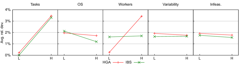
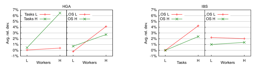
Figure 1: Main effects (upper row) and most significant double interactions (lower row) for HGA and IBS of the five experimental factors on average relative deviations.

A statistical analysis shows that the most significant factors influencing the average solution quality of HGA and IBS are the number of tasks and workers, and the order strength. Figure 1 shows the main effects and interaction plots for the two most significant double interactions for HGA and IBS. The solution quality of both methods strongly depends on the number of tasks. IBS performs better for low order strength, and the HGA performs significantly better when the number of workers is low. These dependencies are more pronounced for a high number of tasks.

In summary, the approach using a HGA seems adequate for obtaining good solutions, with results comparable to or better than the existing heuristics. In particular it obtains significantly better solutions for a low number of workers. Being a relatively simple method, optimizing the task priorities of a station-based assignment scheme inside a generic hybrid genetic algorithm, the HGA may be an interesting alternative for solving the ALWABP-2.

6 Conclusions

In this paper, we have proposed a constructive heuristic framework based on task and worker assignment priority rules for the assembly line worker assignment and balancing problem. In a series of computational tests, the approach proved to be fast and efficient both when evaluated as a stand-alone method as well as when the obtained solutions were used to improve the convergence of more elaborate meta-heuristics. Moreover, the strategy was used as a solution decoder within a hybrid genetic algorithm which was also proposed and tested, obtaining results that were comparable to the best known methods available in the literature.

References

- Baybars (1986) Baybars I (1986) A survey of exact algorithms for the simple assembly line balancing problem. Manag Sci 32:909–932
- Bean (1994) Bean JC (1994) Genetic algorithms and random keys for sequencing and optimization. ORSA J Comp 6:154–160
- Blum and Miralles (2011) Blum C, Miralles C (2011) On solving the assembly line worker assignment and balancing problem via beam search. Comp Oper Res 38:328–339
- Boysen et al (2007) Boysen N, Fliedner M, Scholl A (2007) A classification of assembly line balancing problems. Eur J Oper Res 183:674–693, DOI 10.1016/j.ejor.2006.10.010
- Boysen et al (2008) Boysen N, Fliedner M, Scholl A (2008) Assembly line balancing: Which model to use when? Int J Prod Econ 111:509–528, DOI 10.1016/j.ijpe.2007.02.026
- Chaves et al (2007) Chaves AA, Miralles C, Lorena LAN (2007) Clustering search approach for the assembly line worker assignment and balancing problem. In: Proc. of the 37th International Conference on Computers and Industrial Engineering, Alexandria, Egypt, pp 1469–1478
- Chaves et al (2009) Chaves AA, Lorena LAN, Miralles C (2009) Hybrid metaheuristic for the assembly line worker assignment and balancing problem. Lecture Notes on Computer Science 5818:1–14
- Goldberg (1989) Goldberg DE (1989) Genetic Algorithms in Search, Optimization, and Machine Learning. Addison-Wesley
- Gonçalves and de Almeida (2004) Gonçalves JF, de Almeida JR (2004) A hybrid genetic algorithm for assembly line balancing. J Heuristics 8(6):629–642
- Holland (1975) Holland JH (1975) Adaptation in Natural and Artifical Systems. MIT Press, Cambrigde, MA.
- Klein and Scholl (1999) Klein R, Scholl A (1999) Computing lower bounds by destructive improvement – an application to resource-constrained project scheduling. Eur J Oper Res 112:322–346
- Mendes et al (2009) Mendes JJM, Gonçalves JF, Resende MGC (2009) A random key based genetic algorithm for the resource constrained project scheduling problem. Comp Oper Res 36(1):92–109
- Miralles et al (2007) Miralles C, Garcia-Sabater JP, Andrés C, Cardos M (2007) Advantages of assembly lines in sheltered work centres for disabled. A case study. Int J Prod Econ 110:187–197
- Miralles et al (2008) Miralles C, Garcia-Sabater JP, Andrés C, Cardos M (2008) Branch and bound procedures for solving the assembly line worker assignment and balancing problem: Application to sheltered work centres for disabled. Discrete App Math 156:352–367
- Moreira and Costa (2009) Moreira MCO, Costa AM (2009) A minimalist yet efficient tabu search for balancing assembly lines with disabled workers. In: Anais do XLI Simpósio Brasileiro de Pesquisa Operacional, Porto Seguro
- Scholl (1999) Scholl A (1999) Balancing and sequencing of assembly lines. Physica-Verlag
- Scholl and Becker (2006) Scholl A, Becker C (2006) State-of-the-art exact and heuristic solution procedures for simple assembly line balancing. Eur J Oper Res 168(3):666–693
- Scholl and Voß (1996) Scholl A, Voß S (1996) Simple assembly line balancing – heuristic approaches. J Heuristics 2:217–244, DOI 10.1007/BF00127358
- Talbot et al (1986) Talbot FB, Patterson JH, Gehrlein WV (1986) A comparative evaluation of heuristic line balancing techniques. Manag Sci 32(4):430–454