Blazar 3C 454.3 in Outburst and Quiescence During 2005-2007:
Two Variable Synchrotron Emission Peaks

Abstract

We monitored the flaring blazar 3C 454.3 during 2005 June-July with the Spitzer Infrared Spectrograph (IRS: 15 epochs), Infrared Array Camera (IRAC: 12 epochs) and Multiband Imaging Photometer (MIPS: 2 epochs). We also made Spitzer IRS, IRAC, and MIPS observations from 2006 December-2007 January when the source was in a low state, the latter simultaneous with a single Chandra X-ray observation. In addition, we present optical and sub-mm monitoring data. The 2005-2007 period saw 3 major outbursts. We present evidence that the radio-optical SED actually consists of two variable synchrotron peaks, the primary at IR and the secondary at sub-mm wavelengths. The lag between the optical and sub-mm outbursts may indicate that these two peaks arise from two distinct regions along the jet separated by a distance of 0.07-5 pc. The flux at 5-35 $\mu$m varied by a factor of 40 and the IR peak varied in frequency from $<1\times 10^{13}$ Hz to $4\times 10^{13}$ Hz between the highest and lowest states in 2005 and 2006, respectively. Variability was well correlated across the mid-IR band, with no measurable lag. Flares that doubled in flux occurred on a time scale of $\sim 3$ days. The IR SED peak moved to higher frequency as a flare brightened, then returned to lower frequency as it decayed. The fractional variability amplitude increased with frequency, which we attribute to decreasing synchrotron-self absorption optical depth. Mid-IR flares may signal the re-energization of a shock that runs into inhomogeneities along the pre-existing jet or in the external medium. The synchrotron peak frequencies during each major outburst may depend upon both the distance from the jet apex and the physical conditions in the shocks. Variation of the Doppler parameter along a curved or helical jet is another possibility. Frequency variability of the IR synchrotron peak may have important consequences for the interpretation of the blazar sequence, and the presence of a secondary peak may give insight into jet structure.

1. Introduction

In 2004 August - 2005 September, the blazar 3C 454.3 (z=0.859) underwent the largest radio-optical flare in its recorded history. In 2005 May, it briefly surpassed 3C 273 as the optically brightest quasar in the sky in spite of its much greater distance. This flaring event was intensively monitored at all frequencies by observers all over the world, using both ground and space-based observatories (Villata et al., 2006; Pian et al., 2006; Fuhrmann et al., 2006; Villata et al., 2007; Raiteri et al., 2007). The source has since flared twice again with smaller amplitude, offering continuing opportunities to study this spectacular phenomenon, e.g., Villata et al. (2009); Hagen-Thorn et al. (2009); Vercellone et al. (2009a); Raiteri et al. (2008a, b).

Blazars, including flat-spectrum radio-loud quasars and BL Lac objects, are characterized by strong variability and high polarization. According to active galaxy unification models, they are viewed within $\sim 20\arcdeg$ of the radio jet axis. The spectral energy distribution (SED) is dominated by relativistically boosted emission from the core of the jet. The core is strongly variable at all frequencies, owing to rapid movement and changes in the jet on sub-parsec scales. Very-long baseline interferometry typically shows jet components with apparently superluminal motion at milliarcsecond resolution, demonstrating the importance of relativistic effects.

The SEDs of blazars are typically characterized by two major bumps, one which peaks in the radio through X-ray bands, and the other which peaks in X-$\gamma$ ray bands. The low frequency bump is highly polarized, indicating synchrotron emission from relativistic electrons in a magnetized jet. The high frequency bump is thought to be produced by inverse-Compton scattering of photons by relativistic electrons. However, the source of the photons is a subject of debate, ranging from the synchrotron photons in the jet itself to external photon fields (e.g., Wehrle et al., 1998). In some blazars, a significant fraction of the optical-UV thermal emission as well as broad optical-UV emission lines may arise from an accretion disk (Smith et al., 1988). See, for example, Ghisellini & Tavecchio (2009) and references therein, for a review of models and their application to the class of flat spectrum radio quasars.

Theoretical unifying schemes for $\gamma$-ray bright blazars have been proposed: the more luminous the blazar, the lower the peak frequencies of the synchrotron and Compton bumps (Fossati et al., 1998; Ghisellini et al., 1998). Physically, the down-shift in peak frequency can be caused by increased Compton cooling at higher radiation densities. According to the external-Compton (EC) model, photon fields from the accretion disk, broad-line region (BLR), and dusty torus act to sap energy from the relativistic jet. Hence, luminous flat-spectrum radio quasar (FSRQ) SEDs peak (on average) at lower frequencies than do those of BL Lac objects. Similarly, we might expect accretion disk luminosity variations in a single object to be accompanied by changes in the frequency of the synchrotron peak.

However, Compton cooling may be counterbalanced by re-acceleration of high energy electrons in jet shocks. As a disturbance travels down the jet, it may run into inhomogeneities internal to or external to the jet. At such locations, the bulk relativistic kinetic energy and energy in the electromagnetic field is dissipated, heating the electrons, which emit copious synchrotron photons as they gyrate about the magnetic field lines. The increased number of high energy electrons will shift the synchrotron peak to higher frequencies. Thus the peak synchrotron frequency is determined by a balance between shock heating and Compton cooling, and should vary as jet shock components evolve. An exact correspondence between accretion luminosity and peak synchrotron frequency is therefore not expected.

The IR is a crucial band since it covers the primary synchrotron emission peak of FSRQs, which may provide seed photons for the Compton $\gamma$-ray bump. In addition, while the base of the jet is optically thick at radio frequencies, it is optically thin at mid-IR through UV frequencies. Thus IR observations are less subject to optical depth effects than radio observations and can be used to probe short variability time scales which arise close to the origin of the jet. If flaring episodes are caused by shocks (Marscher & Gear, 1985), then flares should occur simultaneously across the IR through UV wavebands (Lainela, 1994; Savolainen et al., 2002). Therefore, IR spectral variability should reflect changes in the energy distribution of relativistic electrons. Variability on day to month time scales can be used to study the evolution of the shock as it propagates along the jet and through the environment of the active galactic nucleus.

The blazar 3C 454.3 has undergone a number of flaring episodes, with bright radio outbursts occurring roughly once every 6 years (Ciaramella et al., 2004). It has a one-sided milliarcsecond scale radio jet (Pearson, Readhead, & Wilkinson, 1980; Cawthorne & Gabuzda, 1996; Marscher et al., 2002; Scott et al., 2003). Very Long Baseline Interferometric (VLBI) monitoring observations reveal a series of jet components, including stationary components and components with apparent superluminal motion of up to 16 $h^{-1}c$ (Pauliny Toth et al., 1987; Gomez, Marscher, & Albierdi, 1999; Jorstad et al., 2001; Kellerman et al., 2004).

Historically, the synchrotron emission from 3C 454.3 typically peaks in $\nu F_{\nu}$ in the far-IR ($\sim 100$ $\mu$m). IR emission observed by ISO had a flux of 34 mJy at 12.8 $\mu$m (Haas et al., 2004). Excess emission in the SED at 60 $\mu$m was attributed to thermal emission from 100 K dust by these authors, but we will present evidence that this emission is highly variable. The X-ray spectrum observed with Beppo-SAX was characterized by an 0.5-200 keV power law with spectral index $\alpha=-2.3$ (Tavecchio et al., 2002).The greatest amount of energy is emitted in the Compton bump, which peaks at $\sim 10$ MeV. Gamma-ray emission was observed at energies of 0.05-4 GeV by the EGRET and OSSE instruments on the Compton Gamma-Ray Observatory (Hartman et al., 1993; McNaron-Brown et al., 1995; Zhang et al., 2005). Gamma-ray detections after the data in this paper were obtained include those by AGILE (Vercellone et al., 2009a) in 2007, by the LAT instrument on Fermi in 2008 (Abdo et al., 2009), and by AGILE in 2008-2009 (Donnarumma et al., 2009a); see also the review by Vercellone et al. (2009b).

We were awarded director’s discretionary time to observe 3C 454.3 daily with the Spitzer Infrared Spectrograph (IRS), the Infrared Array Camera (IRAC), and the Multiband Imaging Photometer (MIPS) over a period of 4 weeks in 2005 July, during normally scheduled instrument campaigns. We also took coordinated Spitzer MIPS, IRS, IRAC and Chandra High Energy Transmission Grating (HETG) observations in 2006 December -2007 January. We obtained observations from long term optical monitoring programs at Colgate University and Palomar Observatory and from calibrator monitoring at the Submillimeter Array (SMA). In this paper, we present these data and discuss variability and the nature of synchrotron emission flares from the blazar 3C 454.3.

2. A Brief History of 3C 454.3 in 2005-2007

Observations that were made during the same time period as those reported in this paper included several large multiwavelength campaigns, summarized here. Following the alert of an optical flare in 3C 454.3 by Balonek (2005a) and Balonek (2005b), Fuhrmann et al. (2006) obtained near-IR/optical photometry starting two days later. Villata et al. (2006) made the first report of the WEBT multiwavelength campaigns, including ToO pointings by Chandra and Integral, that followed the discovery of the May 2005 optical flare. Raiteri et al. (2007) reported the detection of the ”small and big blue bumps” during the low state in 2006. Villata et al. (2007) derived the delay between centimeter-band radio and optical light curves during 2005-2006. Giommi et al. (2006) observed 3C 454.3 with the robotic Rapid Eye Mount optical/near-infrared telescope and with the Swift satellite in April-May 2005. Raiteri et al. (2008a) presented multifrequency observations by the WEBT and XMM-Newton in 2007-2008, overlapping with AGILE’s November 2007 observations. They also used 1.3 mm monitoring data from the SMA, some of which is also used in our paper, over the time period 2005-2008 (see their Figure 4) as well as 1.3 mm data from Pico Veleta, Spain. X-ray data from Swift, Chandra, XMM-Newton, and Integral data from the 2005-2007 period have been presented by Giommi et al. (2006), Villata et al. (2006), Raiteri et al. (2007) and Pian et al. (2006). We describe the results of these papers as follows.

1. Fuhrmann et al. (2006) observed 3C 454.3 with the Automatic Imaging Telescope of Perugia University Observatory and the Rapid Eye Mount telescope in Chile, obtaining V,R,I and H band photometry. The spectral index over these bands showed no strong significant changes.

2. Villata et al. (2006) presented results up through September 2005, finding that the source was redder when brighter. A mm outburst occurred in June-July 2005, followed months later by the 37-43 GHz peak. Chandra and Integral X-ray observations in May 2005 showed unusually high fluxes.

3. Giommi et al. (2006) observed 3C 454.3 with the robotic Rapid Eye Mount optical/near-infrared telescope and with the Swift satellite in April-May 2005. They found that the optical and ultraviolet flux doubled within a single $1.5\times 10^{5}$ second exposure, the XRT (2-10 keV) X-ray flux varied little during the same time. However, on time scales of a few days, the BAT (15-150 keV) X-ray flux varied by more than a factor of three; in contrast, the average level of the optical-ultraviolet flux was approximately constant between the two UVOT observations of 24 April and 17 May 2005.

4. Villata et al. (2007) reported multiwavelength observations during 2005-2006. Their analysis suggested that the big radio flare (43-37 GHz) in early 2006 was associated with a minor optical flare in October-November 2005, not with the spring 2005 major optical flare. A combination of disturbances traveling down the jet and changes of viewing angles of different emitting regions, with concomitant changes in Doppler boosting, were found to explain the radio delays with respect to the optical emission.

5. Raiteri et al. (2007) detected the ”small and big blue bumps” during the low state in 2006. Observations from K-band through ultraviolet showed a small peak in optical band (V), an upturn in ultraviolet from U-band to UVW1 and UVM2 and an upturn at the infrared end. The infrared end was probably variable synchrotron emission, complicated by a non-variable H-alpha line (reported by Raiteri et al. (2008a) via spectroscopy in J band). The ”small blue bump” is probably a blend of iron lines, Mg II lines and Balmer continuum from the broad line region. The ultraviolet upturn, interpreted as the beginning of the big blue bump was probably from thermal emission of the accretion disk. All these physical emission mechanisms contributed during various activity levels. The underlying accretion disk and broad line contributions were visible most clearly when the synchrotron emission was at low ebb. The X-ray spectra could be fitted with a power law, but seemed to require extra $N_{H}$ absorption some of the time. Alternatively, there may have been spectral changes in the soft X-ray range.

6. Raiteri et al. (2008a) presented multifrequency observations by the WEBT and XMM-Newton in 2007-2008, overlapping with AGILE’s November 2007 observations. They also used 1.3 mm monitoring data from the SMA, some of which is also used in our paper, over the time period 2005-2008 (see their Figure 4) as well as 1.3 mm data from Pico Veleta, Spain. Correlation of the WEBT R-band optical data with the SMA and Pico Veleta data showed that the millimeter fluxes lagged the optical fluxes by 40-80 days, with Discrete Correlation Function maximum signal at 65 days. Taking only non-outburst data for the correlation yielded a DCF maximum at 20 days. They suggested that the “jet regions emitting the optical and mm radiations are now better aligned than in the past, and/or that the opacity in the jet has decreased, allowing the release of mm radiation closer to the optically emitting zone.” We return to this correlation later in our paper. Several multiwavelength SEDs during 2005-2007 are shown and analyzed. From the X-ray-optical correlation, they found that the X-ray, near-infrared and optical emission would be produced in the same spatial region.

3. Observations

3.1. Submillimeter Array Observations

The Submillimeter Array (SMA) is an 8-element radio interferometer located atop Mauna Kea, Hawaii, which operates in the 1.3 mm, 850 $\mu$m, and 450 $\mu$m atmospheric windows (Ho et al., 2004). In the 1.3 mm and 850 $\mu$m windows, quasars are utilized as amplitude and phase gain calibrator sources during routine observing, and the flux density scale is derived through observations of standards in each session, typically solar system sources (with Uranus, Neptune, Titan, Ganymede and Callisto being the most used). The SMA supports a program to calibrate quasar flux densities using both routine science and dedicated calibration observations, and provide their histories to SMA users and the wider astronomical community. The Submillimeter Calibrator List, containing the flux measurement histories of several hundred quasars, can be found in the Tools section of the SMA Observer Center , with further details provided by Gurwell et al. (2007). Data for 2005-2007 are presented in Table 1 and Figure 1 for the 850 $\mu$m and 1 mm bands.

3.1.1 Submillimeter Flares

The sub-mm data, shown in Figure 1a, show a huge flare peaking at 42.7 Jy on 2005 June 24 and a smaller flare of 20 Jy in February 2006. Figure 1b shows the extraordinary flare in 2005 and a surprisingly large amount of substructure during the 2-month period around the peak, including five dates on which the flux exceeded 40 Jy. We think the substructure is real rather than random noise because the variability correlates well between the 230 and 345 GHz band measurements with several measurements in a row showing consistent increasing or decreasing flux density. We can not completely exclude systematic error, for example, observer bias in knowing what the preceding measurement value was.

The SMA is sensitive to only a single polarization which also rotates on the sky as a function of elevation. Anecdotal reports by other observers indicated that 3C 454.3 was not polarized more than a couple of percent. Given the complex rotation relative to the source, it is unlikely that any significant structure in the time variability would be related to changes in the polarization angle, but it cannot be excluded without considerable extra work beyond the scope of this paper.

For about 98% of the measurements, the frequency quoted is in fact the local oscillator (LO) frequency, and the flux measurement is the average of the lower and upper sideband values (in the heterodyne mixing, the sky frequencies are mixed down to the more manageable IF frequency range of 4-6 GHz, but we accept both sidebands, e.g. LO +/- (4-6 GHz). The use of interferometry and the complex correlator allows us to unambiguously separate the sidebands, so we really get two flux measurements, separated by 10 GHz. The SMA 3C 454.3 data yield a spectral index that typically lies near $\nu^{-0.5}$, thus we would expect only a 2% drop in flux from 220 to 230 GHz (1.3 mm band), and only 1.5% from 335 to 345 GHz (850 $\mu$m band). The peak substructure in the sub-mm flare is definitely not caused simply by changes in the frequency of observation.

3.2. Spitzer Observations

We observed 3C 454.3 with Spitzer IRS, IRAC, and MIPS at several epochs during 2005-2007 (Tables 2 and 3). Note that the three instruments were operated separately (according to their regularly scheduled campaigns of typical length 1-2 weeks) so we do not have simultaneous coverage in the respective IR bands. First, we observed the source once per day from 2005 June 30 - 2005 July 27 to track mid-IR spectral variability following the 2005 May outburst. We conducted a series of 14 daily IRS observations between 2005 June 30 and July 12, followed by 12 daily IRAC observations between July 14 and July 26, followed by two MIPS observations on July 27, the last day of the Spitzer visibility window. We observed the source again on 2006 Dec 20 - 2007 Jan 1, the first of two coordinated Spitzer and Chandra observation sequences (the second is reported by Wehrle et al. 2010, in preparation). We made an observation with IRS on 2006 Dec 20, with IRAC on 2006 Dec 25 and with MIPS on 2007 January 01, the latter simultaneously with Chandra as part of a program unrelated to the flare. All IRS observations were made in staring mode, and IRAC and MIPS images were taken in mapping modes. Parameters of the observations are given in Tables 2 and 3.

3.2.1 IRAC

The IRAC images (Fig. 2) on 2005 July 14 (bright state) and 2006 Dec 25 (faint state) show the unresolved quasar in a field of stars and foreground galaxies. The Spitzer Science Center (SSC) pipeline mosaic data (version 14.0.0) were used for aperture photometry carried out with SSC APEX software package in beta release which was the only Spitzer software available for photometry when we began this work. The apertures used were 2, 4, 5, and 5 pixels in radius (1 pixel = 1.2 arcsecond) at 3.6, 4.5, 5.8 and 8.0 $\mu$m, and corrected using the values given in Table 5.7, p. 53 of the IRAC Data Handbook, Version 3.0. We cross-checked the computed quasar fluxes for a range of apertures with those of a nearby star of roughly comparable brightness; the errors are consistent with the 1.5% systematic errors plus 3% absolute calibration uncertainty of the IRAC (Reach et al., 2005). Despite the unpredictable brightness of the source, none of the IRAC images were saturated. Following the release of a new version of IPAC’s Skyview software (courtesy of B. Hartley (IPAC)), we used it to reduce the images independently. The APEX and Skyview results agree to within two percent, except on 2005 July 14, where the APEX value exceeds the Skyview value by 10% at 3.6 $\mu$m. The Skyview fluxes at 3.6, 4.5, 5.8, and 8 $\mu$m are listed in Table 4.

Serendipitously, during the faint state, the 3.6 and 4.5 $\mu$m IRAC images displayed a faint, 10-$\sigma$ feature about 6 ” from the quasar at PA $\sim 150$ degrees. IRAC detections have been made of arcsecond-scale jets from other blazars, however, this feature appeared on the opposite side from the 8” radio jet at PA -45 degrees (e.g., Cooper et al., 2007). The feature was present in all individual frames when the source was faint, including those from another of our Spitzer programs. It was not associated with typical IRAC instrumental artifacts (J. Surace, private communication). Working with Marco Chiaberge, we pulled archival ACS Hubble images (F. Tavecchio, PI) of the source during a faint episode in August 2004, and found a plausible identification of the IRAC feature with two galaxies, conflated by the much larger IRAC PSF. The galaxies’ brightness and colors indicated that they could be located at roughly the same distance as 3C 454.3 (W.C. Keel, private communication). Figure 3 shows the IRAC and Hubble images side by side.

3.2.2 MIPS

The MIPS images (Fig. 4), taken when the source was bright on 2005 July 27 at 01:48 UT and 15:11 UT, and when the source was faint on 2007 January 1, show the unresolved quasar. In the full 24 $\mu$m images, the bright quasar and a few faint galaxies were visible. At 70 $\mu$m, the quasar was isolated on fairly smooth background. The first Airy ring is clearly visible in each image. In the 2005 July 27 datasets, evidence of ”soft saturation” was found in the 160 $\mu$m data (the pipeline images showed a doughnut-like structure instead of a smooth peak). Special MIPS custom processing on the BCD-level data was performed to obtain useful fluxes by MIPS Instrument Team member K. Gordon (see Gordon et al. (2005) for software description). For 24 and 70 $\mu$m data, the pipeline mosaic data (version 13.2.0) was adequate for our use. The 2007 Jan 01 data were not affected by soft saturation; we used pipeline data (version 13.2.0). The IPAC Skyview analysis package was used for aperture photometry. At 24 $\mu$m, we used a 13” radius aperture and applied an aperture correction of 1.164 (Table 3.13, p. 33 of MIPS Data Handbook version 3.2). At 70 $\mu$m, we used 35” radius aperture and applied an aperture correction for a $\nu^{-2}$ spectral index of 1.197 (Table 3.14, p. 33, MIPS Data Handbook version 3.2). For our 160 $\mu$m data on 2007 Jan 1, we used 50” radius aperture and applied an aperture correction of 1.470 (Table 3.16, p. 35, MIPS Data Handbook v. 3.2).

The fluxes on 2005 July 27 at 01:48 UT and 15:11 UT at 24 $\mu$m were $1.12$ and $1.16$ Jy, at 70 $\mu$m, both epochs’ fluxes were $3.51$ Jy and at 160 $\mu$m, $5.43$ Jy, with systematic errors of 10%, 10% and 20% respectively. The fluxes on 2007 Jan 01 at 24, 70 and 160 $\mu$m were $0.060$ Jy and $0.189$ Jy and $0.22$ Jy, with systematic errors of 10%, 10% and 30% respectively.

Additional confidence in the Spitzer low state 160 micron flux density of 0.22 Jy with 30% systematic uncertainty, measured on 2007 Jan 1, is provided by the completely independent Infrared Space Observatory Photometer measurements while the quasar was in an earlier low state: ISO-Phot measured the 120 and 180 micron flux densities of 0.187 and 0.248 Jy on 1997 December 18 (Haas et al., 2004). ISO-PHOT and Spitzer MIPS were calibrated using different primary and secondary calibrators, including asteroids. The 3C454.3 maps made by ISO and Spitzer were in different orientations on the sky.

3.2.3 IRS Low Resolution

IRS was used in standard staring mode to take low-resolution spectra with the Short-Low (SL2,1) and Long-Low (LL2,1) modules (Figs. 5-6). Because of the unexpectedly bright flux level, digital saturation occurred in some of the 2005 July exposure ramps. This effect is automatically corrected for in the data reduction pipeline by throwing out the saturated samples, leading to lower effective exposure time for the brightest pixels and a corresponding reduction in S/N. Several pixels in the LL1 order of the epoch 14 spectrum had only 2 unsaturated samples in each ramp, leading to the noise spike at 22 $\mu$m (Fig. 5). To guard against this problem, we reduced the exposure times and increased the number of exposures in subsequent epochs.

Spectral reductions began from the Basic Calibrated Datasets (BCDs), which have been processed using the Spitzer S15.3.0 pipeline. The pipeline applied subtraction of dark current, ramp fitting, and nonlinearity, droop, and stray-light corrections. The 2D BCD spectra were median-averaged at each of the two standard nod positions and off-source sky background was subtracted. Radiation-damaged ”rogue” pixels were interactively selected and median-filtered from the 2D spectra using the IRSCLEAN program. Spectra for each nod position were extracted using standard tapered windows (SL2: $7\farcs 2$ at 6 $\mu$m, SL1: $14\farcs 4$ at 12 $\mu$m, LL2: $20\farcs 4$ at 16 $\mu$m, LL1: $34\farcs 4$ at 27 $\mu$m). Finally, spectra from the two nod positions were averaged.

We have devised a fringe-correction algorithm to ameliorate spectral fringes in the LL spectra. The wavelengths of the detector fringes depend on where exactly the source is placed in the slit, which varies with the pointing error of the telescope. The detector fringe patterns were extracted from flat field images and used to derive fringe correction functions. The fringe spectrum was shifted and divided by itself to generate a correction curve to minimize the residual fringes in the source spectrum. This procedure reduced the residual fringe amplitudes from $<4\%$ to $<2\%$ in LL.

We found significant offsets between low-resolution spectral orders, which were likely caused by random pointing offsets. This effect was most pronounced in the SL1 order because of the small size of the slit relative to the telescope point-spread function. Multiplicative corrections of 1.0-1.2 (constant with wavelength) were applied to match the flux in each of the SL2, SL1, and LL2 spectral orders to LL1 to within an accuracy of 1%. The corrections were largest in the epoch 6-8 SL1 spectra (8-20%). For these epochs, there was a residual convex downward curvature of $\sim 3\%$ in SL1 caused by wavelength dependent slit losses, which we did not correct, but which do not affect our conclusions.

We used flux calibrations provided by the SSC, employing low-order polynomial fits to standard star observations to convert from electron s^-1 to Jy. The absolute flux calibration accuracy is limited by the uncertainty of the stellar atmosphere model for the flux calibration standard HR 7341, which is estimated to be $3-5\%$ across the IRS wavelength band (Decin & Eriksson, 2007; Decin et al., 2004). The relative flux accuracy of each epoch is limited by slit losses. Repeatability observations of the standard star HD 173511 give independent 1-$\sigma$ flux calibration uncertainties of 2% for SL2, 1% for SL1 and LL2, and 3% for LL1. After matching all orders to LL1, the relative flux accuracy is 3%. We achieve S/N values of $\sim 60-120$ in the low-resolution spectra, limited by remaining systematic uncertainties in the flat field at a level of $1-2\%$.

We measure the mean flux in five wavebands (Table 5: 5.5-6.5,11.5-12.5, 17-19, 23-25, and 28-32 $\mu$m, observed) from the IRS low resolution spectra. The mean wavelengths for these bands are centered at 6.0, 12.0, 18.0, 24.0, and 30.0 $\mu$m. The light curves for these wavebands are presented in Section 3.2.

There are no emission lines or absorption lines stronger than 2% of the continuum flux in the 2005 June-July low resolution spectra (Fig. 5). There is also no evidence for any significant broad silicate absorption or emission or any emission from polycyclic aromatic hydrocarbons (PAHs). Small deviations of $<2\%$ come from uncertainties in the flux calibration introduced by residual detector fringing effects. The most prominent instrumental feature is a $\sim 10\%$ bump at 14 $\mu$m (the so-called SL1 “teardrop”), which may be caused by scattered light in the detector. There is a similar instrumental bump at 7 $\mu$m and a dip at $\sim 5.5$ $\mu$m, both in SL2 and of unknown origin.

3.2.4 IRS High Resolution

We also took high resolution spectra (Fig. 7) with the Short-High (SH) and Long-High (LH) modules at the beginning and end of the 2005 IRS campaign (June 30 and July 13). These observations were designed to search for any narrow emission or absorption features in the mid-IR spectrum. The high resolution spectra are divided by a factor of 1.04 to match the low-resolution flux calibration, since there is a level mismatch between the two flux standards used in the S15 pipeline to calibrate low and high-resolution data . No sky subtraction was performed. The sky background was small compared to the source flux in SH for the brighter of the two epochs. However, it became significant for the larger LH slit and for the fainter epoch.

We subtracted a second-order polynomial fit to each order of the high-resolution spectra in order to get a closer look at any possible emission line features (Fig. 8). On inspection, it is clear that there is no significant detection at either epoch of any of the following quasar or host galaxy emission features at a redshift of $z=0.859$: [Ar ii], H₂ S(3), [S iv], 11.3 $\mu$m PAH, [Ne ii], [Ne v], [Ne iii], or [S iii]. There is a possible detection of [Ne vi] $\lambda$7.65 $\mu$m at 14.22 $\mu$m. However, it is most likely caused an instrumental defect or noise at the edge of SH order 14.

3.2.5 Comparison of 2005 June-July with 2006 December IRS Observations

The 2005 June-July Spitzer spectra (Fig. 5) were taken more than two months after the peak of the 2005 optical outburst. Even so late after the peak, 3C 454.3 was a factor of $\sim 20$ brighter at mid-IR wavelengths than at any previously published epoch. The peak flux during this period reached 1.14 $\pm 0.03$ Jy at 12 $\mu$m and 2.46 $\pm 0.07$ Jy at 24 $\mu$m (Table 10). The mean spectrum was fit by a power law $F_{\nu}\sim\nu^{-1.2}$ at 6-12 $\mu$m, with an exponential cutoff at longer wavelengths. The primary synchrotron bump peaked at an observed frequency of 1-4$\times 10^{13}$ Hz (30-7 $\mu$m).

In 2006 December, we found 3C 454.3 in a relatively low state (Fig. 6). The low state spectrum is well fit by a simple power law with spectral index $\alpha=1.3$. We find no evidence of emission lines or silicate emission stronger than 3% of the continuum. This suggests that the low-state IR SED is dominated by synchrotron emission from the jet. The flux was 28 $\pm 1$ mJy at 12 $\mu$m, a factor of 40 down from the maximum in 2005 July and slightly fainter than the historical ISO measurement of 34 mJy at 12.8 $\mu$m (Haas et al., 2004).

3.3. Optical Observations

Since 1988, T. Balonek has conducted blazar monitoring observations with Colgate University’s Foggy Bottom Observatory. As described by Kartaltepe & Balonek (2007), observations are made “using a Ferson 16 inch Newtonian/Cassegrain reflecting telescope equipped with a Star I CCD system. The images range in exposure time from 1 to 5 minutes (most images being 2 minutes) and include the B, V, R, and I filters, designed by Beckert (1989) to conform to the Johnson-Cousins system…The images were reduced using standard IRAF packages and customized scripts written to facilitate the data handling for our system.” In the case of 3C 454.3, V, R and I band data were obtained. The photometry for all of the images was calculated using the IRAF apphot package with a 16” diameter aperture and a sky annulus with an inner diameter of 20” and an outer diameter of 40”. Some of the Colgate data were previously shown by Raiteri et al. (2008a). The Foggy Bottom Observatory data, uncorrected for absorption, are listed in Tables 6-8.

Since 2005, the members of the NASA Space Interferometry Mission Key Project on Active Galactic Nuclei, led by A. Wehrle, have conducted blazar monitoring observations using the Caltech automated 1.5m telescope at Palomar Observatory (Cenko et al., 2006). We intensified monitoring of 3C 454.3 when it flared in 2005. Data in filter bands V and R were obtained . Data were reduced with IRAF using aperture photometry, with an 4.56” diameter aperture and a sky annulus of 3.8” radius and 3.8” width. The comparison star sequence is given online and originally by Craine (1977), Angione (1971), Fiorucci et al. (1998), Smith & Balonek (1998), and Raiteri et al. (1998). We used Star H, with V=13.64 and R= 13.10, as the primary comparison star. The Palomar Observatory data, uncorrected for absorption, are given in Tables 9 and 10.

3.4. Chandra Observations

Chandra High Energy Transmission Grating (HETG) observations were taken simultaneously with our Spitzer MIPS observations, for 2.145 ks from 21:35-22:42 UT on 2007 January 1. The grating was used to reduce potential photon pile up  effects on the ACIS-S detector. The data were reduced using standard point-source grating analysis threads under CIAO 4.0. The MEG and HEG $\pm 1$ order grating spectra were grouped to have a minimum of 20 counts/bin. We fixed the hydrogen column density for model fits at $N_{H}=6.5\times 10^{20}$ cm^-2 (Dickey & Lockman, 1990) and assumed standard elemental abundances to estimate Galactic absorption. The best fit to the X-ray continuum was obtained with a single power law of slope $\Gamma=1.53\pm 0.12$ and flux at 2-10 keV of $5.8\pm 0.2\times 10^{-12}$ erg cm^-2 s^-1 ($8.14\times 10^{-4}$ ph s^-1 cm^-2). Adding absorption intrinsic to the host galaxy to the model did not improve the fit. Similar fits were obtained using either $\xi^{2}$ or C-statistics. We report fit parameters using the latter, because of small photon number statistics in spite of grouping the data.

4. Results

4.1. Optical Light Curves

The optical light curves are shown in Figure 9. We scaled the Colgate V band data by 1.15 to match the Palomar V data in constructing the light curves; the discrepancy is probably due to slight mismatches in filters. The optical light curves give the appearance of a series of flares superimposed on an exponential fading of the big flare in 2005 May, with e-folding time of $\sim$ 60 days. The source’s underlying V band flux faded from 23 mJy on about 2005 May 10 to 1.1 mJy on about 2005 September 9. Superimposed flares, numbering about a dozen between May and September, doubled the flux on time scales of 24-48 hours, with similar fade times.

4.2. Infrared Light Curves

The 2005 June-July infrared light curves for IRS and IRAC are shown together with the optical light curves in Figure 9. The IRS portions of these curves are shown in more detail in Fig. 10ab. We compute mean 6-12, 6-24, and 12-24 $\mu$m spectral indices to characterize the spectral hardness Fig. 10c. The photometric variability is similar in all wavebands, with greatest amplitude at the shortest wavelengths. The 6 $\mu$m flux increases by a factor of 2 during 2005 July from $240\pm 20$ mJy at epoch 3, flaring to $470\pm 30$ mJy at epoch 14. All of the dips and peaks in the light curves occur simultaneously at 6, 12, and 24 $\mu$m, to within 0.5 day. There is no measurable lag.

Significant variations are seen in the spectral index as the flux changes in 2005 June - July (Fig. 10). In particular, as the flux increases from epoch 4-5, the slope becomes softer. The flux and spectral slope show only small changes from epoch 5-10. This period is followed by a large flare from epochs 12-14, when the flux increases by 85% at 6 $\mu$m and the spectrum hardens. The flux falls and the spectrum softens again in the epoch after the peak of the flare.

The 6-24 $\mu$m spectral index varies from a maximum of $1.41\pm 0.06$ at epoch 9 to a minimum of $1.17\pm 0.06$ at epoch 13 (Fig. 10). The spectral index uncertainties correspond to the IRS flux repeatability of 2% at 6 $\mu$m and 3% at 24 um, as given in Section 2.2.3. There is an anticorrelation between spectral index and 6 $\mu$m flux (Fig. 11) during 2005 July. The SED becomes harder at high frequencies as the flux increases. The peak of the SED also moves to higher frequency as the flux increses: from $1.8-2.4\times 10^{13}$ Hz to $2.2-4.0\times 10^{13}$ Hz. Whenever the 6 $\mu$m flux increases (epochs 3-4, 7-8, 9-10, 11-14), the spectral index decreases. This is a consequence of the larger variability amplitude at 6 $\mu$m than at 24 $\mu$m. The variability amplitude may be moderated by optical depth to synchrotron self-absorption, which increases with wavelength.

4.3. Correlation of Optical and Infrared Light Curves

An inspection of the optical through infrared light curves (Fig. 9) reveals correlated variability from the V-band to 24 $\mu$m. In particular the epoch 14 flare seen in the IRS light curves (Fig. 10), is seen in all of the optical bands as well. However, a close comparision of the IRAC/IRS 8.0 $\mu$m band with the R-band light curve (Fig. 12) shows significant differences in flaring activity . In particular, the 8.0 $\mu$m band shows a bright flare at days 15-20, following the epoch 14 flare, which is much less pronounced in the R-band. There are clear differences in the relative amplitudes of several other smaller flares, which change continuously with wavelength between the IR and optical bands. This behavior may indicate multiple flaring components in the 3C 454.3 SED which have peak amplitudes at different wavelengths. (See Section 4.4.)

A cross-correlation of the IRAC/IRS 8.0 $\mu$m and R-band light curves shows a pronounced peak with correlation amplitude 0.7 at a lag of $0\pm 0.5$ days (Fig. 12c). This confirms the overall impression that the flaring activity is correlated across the optical and mid-IR bands. However, the cross-correlation curve is broadened, with a secondary peak at a lag of 4 days. This lag is similar to the time between the two brightest 8.0 $\mu$m flares, which may produce an accidental (rather than causal) correlation signal.

4.4. Mid-Infrared- Optical SEDs

The mid-infrared to optical spectral energy distributions are shown in Figure 13. From the Figure, we observe the following.

1) During the period 30 June -13 July 2005, there was less variation at IRS bands than in VRI bands, but during the following ten days, 14 July 2005-25 July, there was more variation at IRAC bands than at VRI, including the 5.8 and 8.0 $\mu$m bands that overlap in wavelength with the IRS.

2) The SED slope over mid-infrared through near-infrared to optical bands was negative in both bright (2005) and faint (2007) states. When the source was a factor of 6-10 weaker (in 2006 July and 2006 December) than it was during our July 2005 observations, Raiteri et al. (2007) observed that the underlying near-infrared-optical (I-R-V bands) SED slope was positive, unlike our 2005 observations. In their data, the optical emission peaked at V, then decreased in Swift B and U bands and rose again at Swift W1 and M2 bands. These data, taken together, are consistent with the Raiteri et al. detection of an underlying ”small blue bump” (probably a blend of iron lines, MgII lines and Balmer continuum from the broad line region) whose V-band-peaked emission is visible only when the synchrotron emission is comparatively faint, and whose signature is overwhelmed by synchrotron emission when the source is flaring 6-10 times brighter. Our observations do not cover the Swift bands which show the rise in thermal emission from the accretion disk.

3) The SED does not rise or fall by a constant amount across the mid-infrared to optical bands from day to day. Moreover, the individual band-to-band spectral indices are not the same from day to day. There is no obvious wavelength range over which we see the beginning and ending points of added emission. That implies the newly injected population of leptons giving rise to the synchrotron emission is broad in energy, but we have to keep in mind that the particles radiating at a given frequency are from both old and new populations. Previously injected populations contribute at lower frequencies long after that population’s high energy electrons no longer radiate at high frequencies, assuming no change in the ambient magnetic field.

4) Energy gained in a day at optical bands can be lost in a day, but it takes longer to both gain and lose energy at mid-infrared bands. We see no evidence of asymmetric rise or fall in the mid infrared or optical flares.

4.5. Comparison of Outburst and Quiescent X-ray Fluxes and Spectral Indices

On 19 May 2005, during outburst and a month earlier than our first Spitzer observations, Chandra observed 3C 454.3 for 112 ksec using the HRC-LETG, as a Target of Opportunity within a program on flaring blazars (F. Nicastro, PI; Villata et al. 2006). The 0.2-8 keV spectrum was fitted with a power law of photon index $\Gamma=1.477\pm 0.017$, with $N_{H}=(1.34\pm 0.05)\times 10^{21}$ cm^-2, more than twice the Galactic value (a misprint in Villata et al. 2006 has been corrected). During our 1 January 2007 Chandra observations, obtained using the HETG mode when the source was quiescent, the 2-10 keV spectral index was quite similar ($\Gamma=1.53\pm 0.12$) using the Galactic $N_{H}$ value of $6.5\times 10^{20}$ cm^-2. The May 2005 de-absorbed fluxes were $F=(5.5\pm 0.2)\times 10^{-11}$ erg cm^-2 s^-1 and $(8.4\pm 0.2)\times 10^{-11}$ erg cm^-2 s^-1 in the 0.2-2 keV and 2-8 keV bands (respectively), compared to the January 2007 flux at 2-10 keV of $5.8\pm 0.2\times 10^{-12}$ erg s^-1. Hence, the 2-10 keV X-ray flux dropped by a factor of $\sim$ 10 while the spectral index remained the same, but the bright state required twice as much $N_{H}$ along the line of sight as the quiescent state. An Integral observation (Pian et al. 2006) made 15-18 May 2005 was fitted with a power law of index ${\Gamma}=1.8\pm 0.1$ using the same (Dickey & Lockman, 1990) Galactic $N_{H}$ value The flux in the band 3-200 keV was $5.45\times 10^{-10}$ erg cm^-2 s^-1.

5. Discussion

5.1. The Spectral Energy Distributions: Two Synchrotron Peaks

We use our multiwavelength photometry and the IRS spectra together in constructing radio-X-ray SEDs (Figure 14); representative data are listed for convenience in Tables 11 and 12. In constructing the SEDs, the photometry was corrected for Galactic absorption at V, R and I bands by 0.355, 0.286, and 0.208 magnitudes, respectively. The Colgate V band data were also scaled by 1.15 to match the Palomar V data, as mentioned above.

During 2005 June 30-July 12 (high state), the primary SED peak fell in the IRS 5-35 $\mu$m band (Fig. 14). Strong variability of the continuum level, slope, and peak frequency are characteristic of synchroton emission from a relativistic radio jet. The largest variability amplitudes are seen in the IRAC 3.6 $\mu$m and near-IR (I) bands and the smallest amplitude at 35 $\mu$m. The turnover and lower variability amplitude at lower frequencies may indicate the onset of optically thick synchrotron emission. Without long-wavelength IR coverage, we lost track of the primary synchrotron peak location during the July 14-26 IRAC campaign. When the MIPS observations picked up on July 27, the IR peak had faded somewhat and shifted to the MIPS 70 $\mu$m band.

In the 2006 December 25-2007 January 2 low state, the IR SED peaked in the MIPS 70 $\mu$m FIR band. The low-state SED was similar to that reported by Haas et al. (2004), and to other low-state measurements from NED published over the period 1979-1995 (Fig. 14). One striking difference was the higher 60 $\mu$m flux measured by Haas et al. (2004), which was $\sim 4$ times greater than our MIPS 70 $\mu$m flux, but less than the 2005 peak. This is additional evidence that the 60 $\mu$m flux is highly variable, and indicates that there was little if any contribution from thermal dust emission during the Haas et al. (2004) observation. It is particularly evident during our low-state Spitzer observations (Fig. 14) that there are two peaks in the radio-IR SED, as seen earlier in the low-state observations, made by combining ISO data from 1996 Dec 12 and 1997 Dec 18, of Haas et al. (2004). As we recall from Section 3.2.2, the veracity of the Spitzer 160 micron flux measurement in 2007 January is backed up by the detection of a similarly low level in 1997 by ISO.

During both the low and high states, the primary SED peak occurs at MIR-FIR wavelengths, depending on source brightness. The secondary peak occurs in the sub-mm, near 850 $\mu$m. Strong variability of both bumps indicates that they are both composed of synchrotron emission from the relativistic jet. At the time of the 2005 July 27 MIPS observations, two bumps are also apparent, with the minimum falling somewhere between 160 $\mu$m and 850 $\mu$m. The sharpest contrast between the two peaks is seen during the ISO epochs, when the infrared peak was defined by the 0.706 Jy peak at 60 $\mu$m.

In contrast, non-blazar quasars have two thermal peaks in their SEDs: an ultraviolet peak from the accretion disk and an infrared peak due to reprocessing of ultraviolet light by a dusty torus. We have plotted the mean Richards et al. (2006) QSO SED, compiled from SDSS, Spitzer, near-IR, GALEX, VLA, and ROSAT data in Figure 14, redshifted and scaled for comparison to the 3C 454.3 low state. The UV thermal peak is matched to the big and small blue bumps observed by XMM OM (Raiteri et al., 2007). The IR bump in the low-state 3C 454.3 SED is significantly redder and peaks at a much lower frequency than the IR bump in the mean QSO SED. A thermal SED that peaks at 70 $\mu$m is difficult to model with a standard dusty torus (e.g., Levenson et al., 2007), and would instead require that the QSO be deeply buried in an optically thick sphere of cold dust, contrary to the lack of any silicate absorption in the MIR spectrum and presence of an unobscured Big Blue Bump (BBB) component in the UV SED.

We can also confidently rule out a significant thermal contribution from cold dust heated by star formation in the host galaxy of 3C 454.3. In Figure 14, we overplot the SED template constructed for a star formation dominated hyper-ULIRG (Rieke et al., 2009) with bolometric luminosity $1\times 10^{13}L_{\odot}$, scaled up by a factor of $2.2$ to match the low-state 70 $\mu$m (isotropic) luminosity of $2.9\times 10^{46}$ erg s^-1. Hyper-ULIRG galaxies are extremely rare in the universe and it would be very unusual for a such a high-luminosity, radio loud, type 1 quasar to have a starburst dominated FIR SED. Furthermore, the low state 5-70 $\mu$m power law with spectral index $-1.3$ ($\S$ 3.2.5) is is much flatter than the spectral index of the template hyper-ULIRG SED. We therefore conclude that the jet provides the dominant contribution to the low-state SED at 70 $\mu$m.

5.2. Interpretation of the 2 Synchrotron Peaks

The presence of two synchrotron peaks has also been seen or suggested in at least 3 BL Lac objects, including BL Lac (Ravasio et al., 2003; Raiteri et al., 2009), Mrk 501 (Villata & Raiteri, 1999), and Mrk 421 (Donnarumma et al., 2009b). The frequencies of the two peaks are in the near-IR to optical and far-UV to X-ray bands for BL Lacs, in contrast to the sub-mm and far-IR for the FSRQ 3C 454.3. Ravasio et al. (2003) suggest four possible explanations for the double peaks in BL Lac: 1) higher than normal ratio of optical to X-ray extinction, 2) bulk Comptonization, 3) Klein-Nishina effect on Compton cooling, and 4) two synchrotron emission regions. We can immediately rule out the first two explanations for the two peaks in 3C 454.3 because they occur at IR and lower frequencies, where extinction is not sufficient and there is no lower energy photon field to bulk-Comptonize to IR frequencies. While the Klein-Nishina effect can flatten the slope at the high-energy end of the relativistic electron energy distribution (e.g., Bottcher et al., 1997), it can not produce the two distinct synchrotron peaks that we observe in 3C 454.3 (Fig. 14). We therefore focus on the scenario of two synchrotron emission regions.

Our observations of 3C 454.3 provide some clues to the relationship between the two (mid-IR and sub-mm) synchrotron emission peaks. First, that both peaks occur in both the high and low states, over a period of 6 months (and also in the 1996-1997 ISO observations) indicates that the jet structures that produce them must persist in both the flaring and quiescent jet states. They are not a transient phenomenon particular to the 2005 jet flaring episode. However, further monitoring at shorter timescales is crucial to elucidate the relationship between the two peaks. Second, the similar flux intensity (in $\nu F_{\nu}$) and factor $\sim 40$ increase in the flux of both synchrotron peaks indicates that they come from regions or components in the near-side jet that have similar Doppler beaming factors ($\delta\sim 10$ from VLBI radio observations; see $\S 1$).

The very dissimilar peak frequencies ($2\times 10^{11}$ vs. $8\times 10^{13}$ Hz), along with the lack of correlated variability at short timescales between the two peaks (Fig. 12) indicates that they are produced in distinct regions of the jet with different physical parameters. The primary mid-IR peak likely comes from a more compact region closer to the base of the jet than the sub-mm peak because of synchtrotron self-absorption. In the 2005 outburst, both regions appear to have responded to a major disturbance traveling along the jet. If the two regions are at different radii along the jet, then relativistic light travel time effects must shorten the apparent time between the disturbance at the first and second regions. The peak of the 2005 optical outburst occured sometime before 9 May 2005 (the start of a WEBT observing campaign). The 2005 July sub-mm flare occured sometime between 16 May and 3 June 2005 $\Delta t\sim 7-25$ days ($>0.5-2\times 10^{6}$ s) after the peak of the optical outburst. Assuming the disturbance travelled down the jet at relativistic speed $v$, arriving first at the IR emission region and second at the sub-mm emission region, then we estimate the distance between the two regions to be

$\Delta r=\frac{\beta c\Delta t/(1+z)}{1-\beta\cos\theta}$

where $\beta=v/c$ and $\theta$ is the jet inclination to the line of sight. In the case where the jet lies directly along the line of sight, and $\beta-1<<1$, this simplifies to $\Delta r\simeq 2\Gamma_{j}^{2}c\Delta t/(1+z)$, where the jet bulk Lorentz factor is $\Gamma_{j}=(1-\beta^{2})^{-1/2}$. Assuming a possible range of $\Gamma_{j}=5-20$ (typical for superluminal blazars) and $\theta\sim 1/\Gamma_{j}=3-11\arcdeg$ for the jet angle to the line of sight inside the beaming cone, then $\beta=0.980-0.9987$, and $\Delta r=0.07-5$ pc.

We consider two possible geometries for the two synchrotron emission regions (Fig. 15). The geometry suggested by Raiteri et al. (2009) for BL Lac is a helical jet, where the emission comes from two blobs moving at different angles to the line of sight, corresponding to different Doppler parameters. However, it is not clear in this picture why there would be two distinct synchrotron blobs rather than 3 or more blobs or a continuous distribution of emission along the helix. Rather, the existence of exactly two synchrotron peaks which are present in both the low and high states suggests a more permanent jet structure.

Another possible geometry for the two synchrotron emission peaks is that the IR peak comes from the base of the jet, where it becomes optically thin to mid-IR photons, while the sub-mm peak comes from a recollimation shock located further down the jet. Such a recollimation shock has been predicted with jet hydrodynamic simulations (Lind et al., 1989), where jet recollimation is caused by magnetic hoop stresses within the jet. This scenario has recently been invoked to explain the stationary (yet optically variable) HST 1 synchrotron emission knot observed in the jet of M87 (Nakamura, Garofolo, & Meier 2010, in preparation). Alternatively, the sub-mm synchrotron emission region may mark a location where the jet runs into an external density enhancement such as the broad-line region.

If two distinct synchrotron-emitting populations of particles are moving with different speeds and orientations to our line of sight, both populations would have to be folded into models that compute the contributions to the spectral energy distribution from synchrotron self-Compton emission, and external Compton emission from the accretion disk, broad line region, and corona, as has been done for a single broken-power-law-distribution population by Vercellone et al. (2009a). The resulting SEDs may show two peaks in the $\gamma$-ray band, corresponding to the two peaks in the infrared and sub-mm bands.

5.3. The Origin of mid-IR Flaring

Our observations may be further interpreted in the framework of the relativistic shock model (Marscher & Gear, 1985). In this model, shocks are introduced at the base of a pre-existing relativistic jet by events in the accretion disk or supermassive black hole ergosphere. Shocks may be produced by an increase of the relativistic electron energy density, bulk flow speed, or changes in the magnetic field configuration. The electron density, energy density, and magnetic field will be enhanced at a shock front, leading to copious synchrotron and inverse Compton emission observed as a bright flare at radio-gamma frequencies.

According to the shock model, the peak of the mid-IR emission comes from a location along the relativistic jet where the shock becomes optically thin to synchrotron self-absorption. As the shock region progresses along the jet and expands, it will become optically thin at progressively lower frequency, and the synchrotron peak will move from the mid-IR into the far IR as it fades. The historical SED (Figure 14) shows that a synchrotron peak at $\sim 10^{12}$ Hz ($\sim 300$ $\mu$m, rest) is more typical of 3C 454.3 in a non-flaring state.

As the shock propagates down the jet, it loses energy primarily through inverse Compton scattering. An increase in the ambient photon density field, e.g. flares from the accretion disk or close-encounters with broad-line clouds would drain energy from the shock via Compton drag. This can not explain mid-IR flaring, though it could certainly cause flaring of Compton X-rays and $\gamma$-rays, as for 3C279 (Wehrle et al., 1998).

The shock may be re-energized as it runs into inhomogeneities in the jet or surrounding interstellar medium and bulk kinetic energy is converted to electron kinetic energy and magnetic fields. This could explain why we see large-amplitude mid-IR flaring with Spitzer two months after the peak of the 2005 May optical flare, after the original shock had propagated away from the energy source at the base of the jet.

Variability on longer time scales could also be caused by changes in the Doppler factor as the shock velocity changes its angle to the line of sight. As pointed out for BL Lac by Raiteri et al. (2009) and for 3C 454.3 by Villata et al. (2007), beaming in a curved jet varies along the jet and boosts the emission from various parts of the jet which are emitting at different frequencies, possibly causing changes in the observed flux and spectral index.

5.4. Shock Parameters for the IR-Optical Emission Region

We use simple arguments to derive rough estimates of the physical parameters of the IR-optical flaring synchrotron emission regions in 2005 July. The source doubled its MIR (6 $\mu$m) flux in 5 days from 2005 July 8-13 (2.7 days in the host galaxy rest frame), giving a variability brightness temperature of $T_{\mathrm{v}ar}=3.0\times 10^{10}$ K, close to the canonical equipartition value of $5\times 10^{10}$ K. The corresponding variability size is $<3.7\times 10^{12}$ cm if the shock has a bulk Doppler parameter of $\delta\sim 10$. This is smaller than the gravitational radius of the supermassive black hole, $R_{G}=1.5\times 10^{13}M_{8}$ cm.

Optical synchrotron emission may be produced when the magnetic field and Lorentz factor of the emitting electrons are in the range $B\sim$1-10 Gauss and $\gamma\sim 10^{3}-10^{4}$. We calculate the e-folding time for synchrotron cooling ($t_{cooling}=2.4\times 10^{9}\gamma_{4}^{-1}B_{\mu G}^{-2}$ yr, where $\gamma_{4}=\gamma/10^{4}$ and B is in units of microGauss) using Eq. 9.23 of Krolik (1999) for B=10 Gauss and $\gamma=10^{4}$ and $10^{3}$ of $\sim$13 minutes and $\sim$ 2 hours, respectively. Both of these values are consistent with variations on timescales of days and an upper limit of one day for the time delay between optical and infrared bands. The overall decline in optical flux on e-folding timescales of six months may be due to adiabatic expansion of a newly emitted or newly coalesced jet component.

6. Conclusions

We have observed 3C 454.3 with Spitzer IRS, IRAC, and MIPS, in a high state in 2005 June-July, two months after the 2005 May optical outburst, and with Spitzer and Chandra HETGS in a low state in 2006 December-2007 January.

We find that:

1) There are no significant narrow or broad emission or absorption features in either the low or high-resolution mid-IR spectra of the high state or low resolution spectrum of the low state, consistent with a dominant nonthermal (synchrotron) emission mechanism during both states.

2) The mid-IR continuum emission is $\sim$ 30 times brighter than during previous ISO observations. The mid-IR flux is highly variable, decreasing by a factor of of 20-40 across the 5-35 $\mu$m band between July 2005 and December 2006, indicating Doppler boosted synchrotron emission from the jet.

3) There are two variable synchrotron emission peaks, one in the sub-mm, and one in the mid-IR. The lack of correlated variability between the peaks on 1-30 day time scales and a lag of 7-25 days between the sub-mm and optical outbursts indicates two separate synchrotron emission regions, separated by $\sim 0.07-5$ pc.

4) The frequency of the primary synchrotron peak varies from $<10^{13}$ Hz to 4$\times 10^{13}$ Hz, moving through the Spitzer IRS bandpass. The peak frequency is higher in outburst than during the low state, consistent with injection of high-energy electrons in a jet shock.

5) The 6-24 $\mu$m spectral slope becomes harder during flares and the peak of the SED moves to higher frequency. This may indicate that the shock is being re-energized as a new jet component runs into inhomogeneities in a slower, preexisting jet or surrounding ISM.

6) No time delay between optical and infrared light curves was observed; any time delay is smaller than 0.5 day. However, there are significant differences between the flaring behavior in the optical and infrared bands. Some flares have larger amplitude in the mid-IR, while others have larger amplitude in the optical.

7) The near-IR -optical spectral slope varies dramatically on the timescale of days, perhaps indicating injection of high energy electrons in jet shocks.

Table 1Submillimeter Array Photometry

Year	Month	Day	UT	MJD	Freq (GHz)	Flux (Jy)	Error (Jy)
2005	01	13	02:57	53383.121	225.6	9.7	0.5
2005	04	26	16:10	53486.672	340.8	18.0	1.1
2005	04	27	15:57	53487.664	340.8	22.2	1.2
2005	05	02	05:36	53492.234	342.5	25.0	1.4
2005	05	06	05:42	53496.238	225.5	25.9	1.3
2005	05	07	07:08	53497.297	340.9	23.9	1.2
2005	05	08	07:16	53498.305	340.8	24.1	1.2
2005	05	09	05:31	53499.230	340.9	24.0	1.3
2005	05	10	04:00	53500.168	340.9	25.1	1.3
2005	05	16	06:21	53506.266	336.6	24.2	1.4
2005	06	03	10:33	53524.441	225.5	42.4	2.1
2005	06	08	05:53	53529.246	342.9	34.9	1.8
2005	06	10	04:24	53531.184	225.5	40.3	2.0
2005	06	13	05:07	53534.215	340.8	29.1	1.5
2005	06	18	12:21	53539.516	342.9	33.7	1.8
2005	06	18	16:44	53539.695	342.9	33.0	1.7
2005	06	20	16:07	53541.672	342.5	35.8	1.8
2005	06	21	05:40	53542.234	271.0	38.0	1.9
2005	06	24	04:12	53545.176	225.4	42.7	2.1
2005	06	26	05:20	53547.223	225.4	41.9	2.2
2005	06	26	14:36	53547.609	225.4	41.8	2.1
2005	06	27	05:25	53548.227	218.4	39.0	2.0
2005	06	28	05:03	53549.211	225.5	35.2	1.8
2005	06	30	08:31	53551.355	225.6	32.1	1.6
2005	07	01	05:20	53552.223	348.7	27.2	1.4
2005	07	02	00:57	53553.039	221.5	34.0	1.7
2005	07	02	10:18	53553.430	225.3	34.2	1.7
2005	07	02	10:18	53553.430	225.3	36.1	1.8
2005	07	03	01:54	53554.078	348.7	32.0	1.6
2005	07	03	10:55	53554.453	342.9	31.6	1.6
2005	07	04	04:58	53555.207	348.7	37.9	1.9
2005	07	04	13:20	53555.555	221.5	41.0	2.0
2005	07	05	00:44	53556.031	348.7	40.4	2.0
2005	07	06	10:00	53557.418	222.6	40.0	4.2
2005	07	06	18:02	53557.750	225.4	41.9	4.3
2005	07	07	13:25	53558.559	348.7	38.2	4.3
2005	07	08	12:35	53559.523	330.2	37.8	4.1
2005	07	08	15:38	53559.652	330.2	37.8	1.9
2005	07	09	12:01	53560.500	348.7	36.1	3.7
2005	07	10	15:04	53561.629	346.9	36.3	1.8
2005	07	12	17:57	53563.746	271.7	35.3	1.9
2005	07	15	17:23	53566.723	271.7	40.6	2.0
2005	07	16	15:04	53567.629	289.6	38.6	2.0
2005	07	17	15:24	53568.641	274.5	35.1	1.8
2005	07	19	13:16	53570.555	215.5	33.0	3.7
2005	07	20	13:23	53571.559	226.9	30.8	1.5
2005	07	21	10:15	53572.426	343.0	27.7	1.4
2005	07	21	14:18	53572.598	343.0	28.4	1.4
2005	07	22	12:58	53573.539	226.9	30.1	1.5
2005	07	22	17:33	53573.730	226.9	31.2	3.5
2005	07	24	14:49	53575.617	225.4	31.3	1.6
2005	07	26	16:21	53577.680	224.9	34.9	1.8
2005	07	27	10:07	53578.422	348.0	32.4	1.8
2005	07	28	15:11	53579.633	226.9	37.0	1.9
2005	07	29	12:41	53580.527	240.0	33.1	1.7
2005	07	30	12:10	53581.508	226.9	33.2	1.7
2005	07	30	15:13	53581.633	226.9	33.6	1.7
2005	07	31	11:46	53582.492	226.9	33.6	1.7
2005	07	31	13:44	53582.570	226.9	33.1	1.7
2005	07	31	16:05	53582.672	226.9	33.0	1.7
2005	08	01	10:37	53583.441	218.1	31.6	1.6
2005	08	01	14:22	53583.598	223.1	32.3	1.6
2005	08	02	13:54	53584.578	221.0	32.9	1.6
2005	08	03	15:56	53585.664	225.6	33.9	1.7
2005	08	04	14:15	53586.594	227.1	35.3	1.8
2005	08	05	11:18	53587.473	225.4	38.0	1.9
2005	08	05	15:23	53587.641	225.4	37.1	1.9
2005	08	06	15:43	53588.656	350.0	29.7	1.5
2005	08	09	15:22	53591.641	224.6	34.9	1.8
2005	08	12	10:52	53594.453	344.6	26.5	1.3
2005	08	19	16:01	53601.668	225.3	27.4	1.4
2005	08	25	12:10	53607.508	338.1	18.9	0.9
2005	08	25	14:46	53607.617	338.1	20.6	1.0
2005	08	26	06:56	53608.289	225.6	27.9	1.7
2005	08	26	11:28	53608.477	225.6	27.1	1.4
2005	09	05	11:58	53618.500	221.4	22.9	1.2
2005	09	06	10:54	53619.453	241.9	19.8	1.0
2005	09	06	13:44	53619.570	223.9	20.9	1.0
2005	09	09	11:06	53622.461	271.0	18.3	1.0
2005	09	09	14:33	53622.605	340.8	13.9	0.7
2005	09	10	11:10	53623.465	226.2	17.6	1.0
2005	09	11	14:12	53624.590	221.3	17.5	0.9
2005	09	12	11:04	53625.461	226.2	17.2	0.9
2005	09	12	13:41	53625.570	225.3	17.1	0.9
2005	09	13	09:52	53626.410	239.1	16.5	0.9
2005	09	17	10:05	53630.422	225.5	14.2	0.8
2005	09	18	10:12	53631.426	239.1	11.8	0.7
2005	10	11	06:09	53654.258	345.0	10.6	0.5
2005	10	20	08:18	53663.348	225.6	13.0	0.7
2005	11	12	05:42	53686.238	222.0	10.4	0.9
2005	11	12	07:01	53686.293	221.9	10.9	0.5
2005	11	22	08:06	53696.336	335.8	9.0	0.5
2005	12	21	07:42	53725.320	225.6	10.7	0.6
2006	01	03	06:10	53738.258	220.3	11.2	0.6
2006	01	07	06:11	53742.258	225.6	12.3	0.6
2006	01	10	01:47	53745.074	348.6	8.4	0.9
2006	01	30	04:49	53765.199	337.7	11.5	0.6
2006	01	31	03:59	53766.164	225.3	14.4	0.7
2006	02	01	19:51	53767.828	225.6	15.8	0.8
2006	02	02	05:16	53768.219	225.3	15.0	0.8
2006	02	03	02:56	53769.121	341.6	11.0	1.2
2006	02	04	04:03	53770.168	221.4	18.5	2.1
2006	02	06	03:52	53772.160	336.5	16.2	0.9
2006	02	07	03:10	53773.133	220.3	17.2	0.9
2006	02	10	19:21	53776.805	224.7	20.1	1.4
2006	02	17	19:52	53783.828	234.8	16.2	1.1
2006	02	24	18:28	53790.770	234.7	17.0	1.0
2006	03	31	22:54	53825.953	225.6	7.7	1.0
2006	04	03	17:28	53828.727	225.5	7.6	0.4
2006	04	06	16:53	53831.703	341.5	6.2	0.3
2006	04	10	17:47	53835.742	347.2	5.4	0.3
2006	04	17	17:26	53842.727	339.7	5.4	0.3
2006	04	18	16:04	53843.668	341.5	5.3	0.3
2006	04	19	16:36	53844.691	338.9	5.4	0.3
2006	04	28	17:16	53853.719	221.4	6.4	0.3
2006	05	01	17:04	53856.711	225.4	5.7	0.3
2006	05	03	13:52	53858.578	234.7	4.7	1.4
2006	05	09	17:08	53864.715	225.5	5.2	0.3
2006	05	16	18:34	53871.773	340.9	3.0	0.2
2006	05	18	15:41	53873.652	225.5	4.8	0.3
2006	05	20	16:04	53875.668	225.6	5.4	0.3
2006	05	21	17:56	53876.746	225.3	5.0	0.3
2006	05	24	17:25	53879.727	234.7	3.8	0.2
2006	05	25	14:42	53880.613	225.3	4.2	0.2
2006	06	07	12:13	53893.508	235.6	3.1	0.2
2006	06	07	18:17	53893.762	235.6	3.1	0.2
2006	06	14	12:55	53900.539	225.6	3.4	0.2
2006	06	15	15:19	53901.637	225.6	3.4	0.2
2006	07	20	10:05	53936.422	225.6	3.2	0.2
2006	07	21	15:13	53937.633	225.5	3.1	0.2
2006	07	28	13:59	53944.582	224.1	3.0	0.1
2006	07	31	16:45	53947.699	223.6	2.8	0.2
2006	08	01	14:00	53948.582	225.5	2.9	0.1
2006	08	03	11:48	53950.492	225.5	3.1	0.3
2006	08	08	13:54	53955.578	225.2	3.2	0.2
2006	08	13	09:01	53960.375	220.8	3.3	0.2
2006	08	14	16:03	53961.668	269.7	2.9	0.1
2006	08	15	14:08	53962.590	225.5	3.5	0.2
2006	08	18	07:53	53965.328	220.6	3.8	0.2
2006	08	24	07:52	53971.328	221.2	3.9	0.2
2006	08	26	12:09	53973.508	225.3	3.9	0.2
2006	09	05	06:30	53983.270	339.3	3.1	0.2
2006	09	08	06:29	53986.270	341.6	3.6	0.6
2006	09	16	12:21	53994.516	225.5	4.2	0.2
2006	09	17	13:01	53995.543	225.3	4.2	0.2
2006	09	18	12:15	53996.512	225.4	4.2	0.3
2006	09	22	08:53	54000.371	341.5	3.6	0.2
2006	09	24	08:50	54002.367	340.0	3.6	0.2
2006	10	04	09:01	54012.375	225.6	4.3	0.2
2006	10	10	05:33	54018.230	225.5	4.3	0.2
2006	10	13	04:45	54021.199	225.3	4.1	0.2
2006	10	13	05:59	54021.250	225.3	4.3	0.2
2006	10	19	07:26	54027.309	220.2	3.8	0.2
2006	10	23	10:24	54031.434	225.5	4.2	0.4
2006	10	24	09:33	54032.398	224.6	4.0	0.2
2006	10	27	08:10	54035.340	220.5	3.8	0.2
2006	11	21	07:00	54060.293	225.5	4.8	0.2
2006	11	23	06:37	54062.277	225.6	4.1	0.2
2006	11	24	06:49	54063.285	271.5	3.9	0.3
2006	11	25	07:48	54064.324	225.2	4.3	0.2
2006	11	28	04:45	54067.199	276.8	3.9	0.2
2006	11	29	06:39	54068.277	213.5	4.6	0.2
2006	12	01	05:34	54070.230	340.8	3.0	0.2
2006	12	09	06:21	54078.266	273.8	3.4	0.2
2006	12	12	08:07	54081.340	343.7	3.3	0.2
2006	12	22	07:22	54091.309	225.5	4.0	0.2
2006	12	29	06:28	54098.270	335.3	2.8	0.2
2007	01	11	06:07	54111.254	225.5	3.5	0.3
2007	01	26	04:25	54126.184	227.8	3.3	0.2

Table 2Spitzer Infrared IRAC and MIPS Observations of 3C 454.3.

Year	Month	Day	Instrument	Waveband ($\mu$m)	Integration Time
2005	07	14-26	IRAC	3.6, 4.5, 5.8, 8	$1\times 32$ s
2005	07	27 (twice)	MIPS	24, 70, 160	$(2,2,4)\times 3$ s
2006	12	25	IRAC	3.6, 4.5, 5.8, 8	$1\times 32$ s
2007	01	02	MIPS	24, 70	$2\times 3$ s

Table 3Spitzer IRS Observations of 3C 454.3.

Epochs	year	month	day	SL	LL	SH	LH
1	2005	06	30	$4\times 60$	$2\times 120$	$4\times 120$	$4\times 60$
2-14	2005	07	01-12	$4\times 60$	$2\times 120$	$0$	$0$
15	2005	07	13	$4\times 60$	$2\times 120$	$4\times 120$	$4\times 60$
16	2006	12	20	$16\times 14$	$24\times 14$	$0$	$0$

Table 4Spitzer Infrared IRAC Photometry of 3C 454.3.

Year	Month	Day	UT	JD	$S_{3.6}[Jy]$	$S_{4.5}[Jy]$	$S_{5.8[Jy]}$	$S_{8.0}[Jy]$
2005	7	14	19:41	2453566.32014	0.172	0.247	0.37	0.616
2005	7	15	17:52	2453567.24444	0.201	0.292	0.445	0.765
2005	7	16	19:41	2453568.32014	0.197	0.282	0.426	0.723
2005	7	17	19:08	2453569.29722	0.239	0.329	0.481	0.774
2005	7	18	21:03	2453570.37708	0.206	0.284	0.417	0.664
2005	7	19	21:17	2453571.38681	0.185	0.258	0.382	0.610
2005	7	20	20:08	2453572.33889	0.163	0.228	0.335	0.533
2005	7	21	20:51	2453573.36875	0.133	0.187	0.277	0.443
2005	7	22	18:49	2453574.28403	0.102	0.145	0.216	0.347
2005	7	23	20:29	2453575.35347	0.092	0.128	0.187	0.293
2005	7	24	08:28	2453575.85278	0.097	0.135	0.198	0.309
2005	7	25	19:49	2453577.32569	0.113	0.156	0.226	0.349
2006	12	25	06:23	2454081.76597	5.65E-3	7.30E-3	9.10E-3	14.2E-3

Table 5Spitzer IRS mid-IR spectrophotometry of 3C 454.3.

Epoch	day	$F_{6}$	$+/-$	$F_{12}$	$+/-$	$F_{18}$	$+/-$	$F_{24}$	$+/-$	$F_{30}$	$+/-$
1	0.0721	0.29	0.02	0.74	0.03	1.26	0.04	1.80	0.05	2.24	0.09
2	1.2601	0.27	0.02	0.68	0.02	1.12	0.04	1.57	0.04	1.91	0.07
3	2.2021	0.24	0.02	0.62	0.02	1.03	0.03	1.45	0.04	1.79	0.07
4	2.9945	0.29	0.02	0.74	0.02	1.22	0.04	1.67	0.04	2.04	0.07
5	4.0043	0.29	0.02	0.79	0.03	1.36	0.05	1.95	0.06	2.45	0.10
6	5.4844	0.27	0.02	0.72	0.03	1.27	0.04	1.86	0.06	2.34	0.09
7	6.3560	0.26	0.02	0.71	0.03	1.25	0.04	1.81	0.06	2.28	0.09
8	7.1905	0.28	0.02	0.76	0.03	1.30	0.05	1.86	0.06	2.34	0.09
9	8.1915	0.26	0.02	0.72	0.03	1.27	0.05	1.83	0.05	2.31	0.09
10	9.0716	0.29	0.02	0.82	0.03	1.40	0.05	1.98	0.06	2.45	0.09
11	10.1821	0.30	0.02	0.79	0.03	1.32	0.05	1.85	0.05	2.28	0.08
12	11.2788	0.37	0.03	0.91	0.03	1.46	0.04	2.01	0.06	2.47	0.09
13	11.9932	0.43	0.03	1.02	0.03	1.60	0.05	2.18	0.05	2.60	0.09
14	12.9880	0.47	0.03	1.14	0.03	1.80	0.05	2.46	0.07	2.95	0.10
15	13.9533	0.37	0.03	0.95	0.03	1.61	0.06	2.27	0.06	2.79	0.10
16	538.5000	0.012	0.001	0.028	0.001	0.047	0.002	0.070	0.003	0.092	0.004

Table 6Foggy Bottom Observatory V-band Observations of 3C 454.3.

Year	Month	Day	UT	Julian Date	V mag	V mag error	Flux [mJy]	Flux error [mJy]
2005	5	9	8:42	2453499.863	12.33	0.031	36.01	1.112
2005	5	10	8:39	2453500.861	12.804	0.031	23.269	0.713
2005	5	13	8:31	2453503.855	13.264	0.032	15.242	0.484
2005	5	17	8:19	2453507.847	13.585	0.035	11.337	0.397
2005	5	19	7:57	2453509.832	12.697	0.029	25.697	0.734
2005	5	21	8:02	2453511.835	13.509	0.034	12.159	0.414
2005	5	26	7:43	2453516.822	13.657	0.027	10.606	0.29
2005	5	28	8:09	2453518.84	13.868	0.047	8.741	0.412
2005	5	30	7:52	2453520.828	13.96	0.045	8.026	0.358
2005	5	31	7:43	2453521.822	14.228	0.063	6.269	0.394
2005	6	1	7:26	2453522.81	14.284	0.053	5.955	0.314
2005	6	2	7:54	2453523.829	14.405	0.072	5.329	0.383
2005	6	3	8:02	2453524.835	14.165	0.22	6.644	1.462
2005	6	5	7:53	2453526.829	14.297	0.05	5.887	0.295
2005	6	6	7:53	2453527.829	14.518	0.098	4.8	0.468
2005	6	7	7:21	2453528.807	14.009	0.047	7.672	0.361
2005	6	8	7:17	2453529.804	13.896	0.046	8.512	0.393
2005	6	10	7:35	2453531.817	13.778	0.078	9.494	0.743
2005	6	11	7:16	2453532.803	13.952	0.111	8.083	0.895
2005	6	15	7:52	2453536.828	14.26	0.07	6.089	0.427
2005	6	20	6:13	2453541.759	13.869	0.032	8.728	0.279
2005	6	21	6:46	2453542.782	14.128	0.051	6.878	0.352
2005	6	23	7:24	2453544.809	13.796	0.035	9.338	0.325
2005	6	24	6:03	2453545.752	14.029	0.048	7.536	0.363
2005	6	25	6:03	2453546.752	14.445	0.074	5.134	0.378
2005	6	26	7:09	2453547.798	14.431	0.066	5.202	0.344
2005	6	27	5:55	2453548.747	14.718	0.085	3.994	0.341
2005	6	28	6:57	2453549.79	14.602	0.04	4.442	0.178
2005	7	1	6:59	2453552.792	14.943	0.06	3.246	0.193
2005	7	3	6:01	2453554.751	14.847	0.031	3.547	0.108
2005	7	4	6:06	2453555.755	14.685	0.043	4.119	0.177
2005	7	4	7:33	2453555.815	14.516	0.051	4.81	0.246
2005	7	5	6:30	2453556.771	14.883	0.089	3.432	0.306
2005	7	11	5:30	2453562.73	13.999	0.055	7.741	0.427
2005	7	12	7:59	2453563.833	14.02	0.031	7.598	0.234
2005	7	14	5:42	2453565.738	14.42	0.042	5.257	0.22
2005	7	15	7:36	2453566.817	14.483	0.051	4.96	0.253
2005	7	16	6:18	2453567.763	14.663	0.054	4.199	0.226
2005	7	20	5:28	2453571.728	14.581	0.041	4.529	0.187
2005	7	21	5:10	2453572.716	14.621	0.05	4.366	0.217
2005	7	22	5:45	2453573.74	14.809	0.053	3.674	0.196
2005	7	23	7:26	2453574.81	15.006	0.039	3.062	0.118
2005	7	26	5:23	2453577.725	14.775	0.037	3.788	0.141
2005	7	28	6:15	2453579.761	14.872	0.032	3.466	0.113
2005	7	29	6:09	2453580.757	14.705	0.031	4.04	0.123
2005	7	31	7:13	2453582.801	14.873	0.041	3.462	0.14
2005	8	2	6:05	2453584.754	15.473	0.123	1.993	0.245
2005	8	3	5:26	2453585.727	15.233	0.045	2.486	0.112
2005	8	4	5:00	2453586.709	15.31	0.09	2.315	0.209
2005	8	6	5:34	2453588.732	15.285	0.042	2.369	0.101
2005	8	7	4:54	2453589.705	15.024	0.039	3.012	0.117
2005	8	8	4:36	2453590.692	15.07	0.044	2.887	0.127
2005	8	10	7:04	2453592.795	15.289	0.043	2.36	0.102
2005	8	17	4:16	2453599.678	15.461	0.052	2.014	0.106
2005	8	17	7:28	2453599.811	15.379	0.049	2.172	0.106
2005	8	25	7:16	2453607.803	14.922	0.025	3.31	0.083
2005	8	27	6:32	2453609.773	15.277	0.038	2.387	0.09
2005	9	2	6:50	2453615.785	15.704	0.055	1.61	0.088
2005	9	4	7:20	2453617.806	15.963	0.062	1.269	0.079
2005	9	5	4:00	2453618.667	15.847	0.053	1.412	0.075
2005	9	6	3:56	2453619.664	15.973	0.057	1.257	0.072
2005	9	8	5:19	2453621.722	15.991	0.061	1.236	0.075
2005	9	10	7:00	2453623.792	16.023	0.097	1.2	0.116
2005	9	11	4:00	2453624.667	15.815	0.052	1.455	0.075
2005	9	12	4:05	2453625.671	16.016	0.068	1.208	0.083
2005	9	24	3:14	2453637.635	15.967	0.052	1.264	0.066
2005	10	3	5:53	2453646.746	15.608	0.053	1.76	0.094
2005	10	4	4:46	2453647.699	15.711	0.054	1.6	0.087

Table 7Foggy Bottom Observatory R-band Observations of 3C 454.3.

Year	Month	Day	UT	Julian Date	R mag	R mag error	Flux [mJy]	Flux error [mJy]
2004	6	21	7:41	2453177.82	15.315	0.019	2.304	0.044
2004	7	7	7:25	2453193.809	15.189	0.048	2.588	0.124
2004	7	21	7:21	2453207.806	15.268	0.052	2.406	0.126
2004	8	22	4:45	2453239.698	15.66	0.042	1.677	0.071
2004	8	25	7:00	2453242.792	15.92	0.134	1.32	0.176
2004	9	5	3:27	2453253.644	14.803	0.029	3.692	0.108
2004	9	12	7:05	2453260.796	15.212	0.045	2.534	0.113
2004	9	14	4:40	2453262.695	14.419	0.017	5.261	0.087
2004	9	19	4:37	2453267.692	14.356	0.015	5.573	0.082
2005	5	9	8:33	2453499.857	11.898	0.007	53.619	0.398
2005	5	9	8:57	2453499.873	11.928	0.024	52.171	1.238
2005	5	10	8:31	2453500.855	12.249	0.008	38.818	0.304
2005	5	13	8:19	2453503.847	12.794	0.009	23.483	0.212
2005	5	17	8:05	2453507.837	13.067	0.009	18.262	0.165
2005	5	18	8:43	2453508.864	12.623	0.016	27.496	0.446
2005	5	19	7:20	2453509.806	12.211	0.009	40.189	0.344
2005	5	19	8:13	2453509.843	12.173	0.007	41.613	0.305
2005	5	21	7:45	2453511.824	12.98	0.007	19.798	0.144
2005	5	21	8:29	2453511.854	12.963	0.011	20.112	0.212
2005	5	26	7:13	2453516.801	13.102	0.006	17.697	0.108
2005	5	26	8:13	2453516.843	13.109	0.009	17.582	0.155
2005	5	27	8:17	2453517.845	13.029	0.025	18.926	0.476
2005	5	28	7:27	2453518.811	13.261	0.021	15.277	0.317
2005	5	30	7:32	2453520.814	13.537	0.012	11.849	0.144
2005	5	30	8:23	2453520.85	13.558	0.012	11.621	0.141
2005	5	31	7:28	2453521.811	13.871	0.038	8.716	0.327
2005	5	31	8:16	2453521.845	13.808	0.011	9.234	0.105
2005	6	1	7:11	2453522.8	13.882	0.016	8.627	0.14
2005	6	1	7:58	2453522.832	13.887	0.015	8.584	0.129
2005	6	2	7:29	2453523.812	13.649	0.015	10.691	0.16
2005	6	2	8:31	2453523.855	13.731	0.042	9.915	0.42
2005	6	3	6:36	2453524.776	13.666	0.028	10.524	0.295
2005	6	3	8:20	2453524.848	13.677	0.077	10.413	0.805
2005	6	5	7:32	2453526.814	13.806	0.015	9.253	0.14
2005	6	6	7:23	2453527.808	13.664	0.018	10.54	0.187
2005	6	6	8:09	2453527.84	13.688	0.02	10.311	0.211
2005	6	7	7:04	2453528.795	13.58	0.014	11.392	0.157
2005	6	7	7:49	2453528.826	13.634	0.014	10.84	0.156
2005	6	8	7:01	2453529.793	13.367	0.013	13.861	0.175
2005	6	8	7:45	2453529.823	13.393	0.013	13.531	0.177
2005	6	9	6:42	2453530.78	13.266	0.016	15.208	0.248
2005	6	10	6:38	2453531.777	13.218	0.019	15.897	0.305
2005	6	10	8:03	2453531.836	13.243	0.017	15.534	0.259
2005	6	11	7:04	2453532.795	13.484	0.026	12.447	0.325
2005	6	11	7:45	2453532.823	13.453	0.023	12.805	0.289
2005	6	13	7:32	2453534.814	13.574	0.024	11.454	0.272
2005	6	15	7:34	2453536.816	13.725	0.015	9.969	0.148
2005	6	16	7:11	2453537.8	13.334	0.018	14.285	0.254
2005	6	20	5:38	2453541.735	13.254	0.01	15.385	0.157
2005	6	20	6:31	2453541.772	13.251	0.01	15.423	0.158
2005	6	21	6:14	2453542.76	13.528	0.014	11.952	0.167
2005	6	21	7:01	2453542.793	13.505	0.013	12.209	0.159
2005	6	23	7:03	2453544.794	13.13	0.01	17.237	0.175
2005	6	23	7:42	2453544.822	13.204	0.009	16.098	0.143
2005	6	24	5:31	2453545.73	13.433	0.014	13.037	0.187
2005	6	24	6:24	2453545.767	13.381	0.012	13.681	0.168
2005	6	25	5:27	2453546.728	13.656	0.019	10.616	0.205
2005	6	25	6:36	2453546.775	13.675	0.017	10.432	0.176
2005	6	26	6:16	2453547.762	13.758	0.034	9.672	0.33
2005	6	27	5:20	2453548.722	14.013	0.024	7.643	0.182
2005	6	27	6:20	2453548.765	14.032	0.022	7.513	0.167
2005	6	28	6:09	2453549.756	14.056	0.024	7.35	0.177
2005	6	28	7:30	2453549.813	14.025	0.019	7.558	0.145
2005	7	1	5:47	2453552.741	14.377	0.032	5.467	0.174
2005	7	1	7:50	2453552.827	14.259	0.038	6.095	0.233
2005	7	2	5:20	2453553.723	14.334	0.084	5.688	0.478
2005	7	3	5:15	2453554.719	14.283	0.02	5.959	0.119
2005	7	3	7:06	2453554.796	14.285	0.012	5.952	0.072
2005	7	4	5:14	2453555.719	14.061	0.021	7.311	0.153
2005	7	4	6:40	2453555.779	14.116	0.016	6.95	0.114
2005	7	5	5:00	2453556.709	14.662	0.087	4.206	0.364
2005	7	5	6:41	2453556.779	14.519	0.029	4.795	0.141
2005	7	10	6:03	2453561.753	14.06	0.022	7.322	0.162
2005	7	11	4:43	2453562.697	13.582	0.016	11.373	0.186
2005	7	11	5:58	2453562.749	13.517	0.01	12.074	0.124
2005	7	12	6:29	2453563.771	13.405	0.015	13.38	0.207
2005	7	12	8:29	2453563.854	13.457	0.015	12.762	0.192
2005	7	14	4:34	2453565.69	13.879	0.017	8.648	0.144
2005	7	14	6:17	2453565.762	13.941	0.025	8.167	0.204
2005	7	15	6:49	2453566.784	13.966	0.028	7.983	0.222
2005	7	15	8:08	2453566.84	13.924	0.022	8.299	0.185
2005	7	16	5:23	2453567.725	13.98	0.028	7.883	0.224
2005	7	16	7:02	2453567.793	14.025	0.02	7.557	0.148
2005	7	19	4:46	2453570.699	14.008	0.05	7.681	0.387
2005	7	20	4:23	2453571.683	14.063	0.023	7.299	0.171
2005	7	20	6:06	2453571.754	14.154	0.021	6.716	0.144
2005	7	21	4:20	2453572.681	14.075	0.02	7.219	0.143
2005	7	21	5:48	2453572.742	14.125	0.017	6.894	0.118
2005	7	22	4:29	2453573.687	14.184	0.025	6.533	0.163
2005	7	22	6:31	2453573.772	14.307	0.019	5.829	0.108
2005	7	23	6:39	2453574.777	14.44	0.025	5.161	0.128
2005	7	23	8:04	2453574.837	14.462	0.019	5.057	0.097
2005	7	24	6:08	2453575.756	14.354	0.03	5.587	0.166
2005	7	24	7:27	2453575.811	14.459	0.026	5.067	0.133
2005	7	26	4:26	2453577.685	14.299	0.019	5.875	0.111
2005	7	26	5:52	2453577.745	14.307	0.017	5.832	0.1
2005	7	28	5:04	2453579.711	14.374	0.041	5.481	0.222
2005	7	28	6:42	2453579.779	14.359	0.021	5.559	0.117
2005	7	29	5:18	2453580.721	14.264	0.017	6.067	0.106
2005	7	30	3:46	2453581.657	14.22	0.024	6.319	0.149
2005	7	31	4:00	2453582.667	14.522	0.062	4.783	0.296
2005	7	31	5:50	2453582.743	14.457	0.032	5.077	0.164
2005	7	31	8:01	2453582.834	14.489	0.034	4.932	0.168
2005	8	1	7:28	2453583.812	14.655	0.033	4.234	0.141
2005	8	2	5:18	2453584.721	14.713	0.041	4.012	0.166
2005	8	3	3:57	2453585.665	14.881	0.039	3.436	0.133
2005	8	3	6:08	2453585.756	14.838	0.03	3.577	0.107
2005	8	3	7:09	2453585.799	14.87	0.033	3.472	0.116
2005	8	3	8:09	2453585.84	14.819	0.027	3.637	0.097
2005	8	3	8:38	2453585.86	14.825	0.028	3.62	0.102
2005	8	4	3:53	2453586.662	14.805	0.035	3.685	0.13
2005	8	4	6:03	2453586.753	14.723	0.031	3.977	0.124
2005	8	5	4:08	2453587.672	14.777	0.099	3.781	0.373
2005	8	6	4:07	2453588.672	14.612	0.034	4.402	0.151
2005	8	6	6:11	2453588.758	14.647	0.021	4.263	0.089
2005	8	7	3:37	2453589.651	14.599	0.013	4.457	0.057
2005	8	7	5:31	2453589.73	14.571	0.017	4.571	0.076
2005	8	8	3:03	2453590.628	14.622	0.017	4.364	0.073
2005	8	8	5:24	2453590.725	14.615	0.011	4.39	0.048
2005	8	8	8:12	2453590.842	14.698	0.015	4.067	0.063
2005	8	9	8:32	2453591.856	14.903	0.031	3.369	0.103
2005	8	10	5:29	2453592.729	14.753	0.013	3.868	0.051
2005	8	10	7:58	2453592.832	14.776	0.018	3.787	0.067
2005	8	11	2:57	2453593.623	14.871	0.066	3.47	0.23
2005	8	16	8:20	2453598.847	14.917	0.048	3.324	0.158
2005	8	17	2:43	2453599.613	14.877	0.016	3.448	0.057
2005	8	17	5:07	2453599.714	14.943	0.016	3.245	0.052
2005	8	17	6:43	2453599.78	14.915	0.015	3.332	0.051
2005	8	17	8:06	2453599.838	14.918	0.014	3.323	0.048
2005	8	18	3:02	2453600.627	15.004	0.026	3.07	0.079
2005	8	23	5:18	2453605.721	15.13	0.023	2.732	0.063
2005	8	24	3:28	2453606.645	14.966	0.024	3.178	0.077
2005	8	25	5:06	2453607.713	14.511	0.007	4.833	0.035
2005	8	25	8:23	2453607.849	14.414	0.008	5.284	0.044
2005	8	26	7:08	2453608.798	14.893	0.034	3.4	0.114
2005	8	27	3:50	2453609.66	14.811	0.013	3.665	0.047
2005	8	27	7:13	2453609.801	14.873	0.016	3.463	0.054
2005	8	29	3:03	2453611.627	14.989	0.021	3.11	0.066
2005	9	2	1:14	2453615.551	15.2	0.026	2.563	0.066
2005	9	2	5:24	2453615.725	15.214	0.017	2.528	0.043
2005	9	2	7:39	2453615.819	15.214	0.02	2.529	0.051
2005	9	3	2:19	2453616.597	15.409	0.023	2.113	0.049
2005	9	3	3:15	2453616.636	15.386	0.019	2.158	0.041
2005	9	3	4:48	2453616.7	15.337	0.025	2.258	0.057
2005	9	4	2:34	2453617.607	15.484	0.027	1.972	0.054
2005	9	4	5:56	2453617.748	15.482	0.027	1.977	0.054
2005	9	4	8:29	2453617.854	15.553	0.026	1.85	0.048
2005	9	5	1:21	2453618.556	15.547	0.022	1.86	0.041
2005	9	5	3:06	2453618.63	15.562	0.019	1.836	0.035
2005	9	5	5:33	2453618.731	15.592	0.017	1.786	0.031
2005	9	6	1:11	2453619.549	15.558	0.023	1.842	0.042
2005	9	6	2:49	2453619.618	15.707	0.024	1.605	0.038
2005	9	6	4:58	2453619.707	15.592	0.02	1.785	0.036
2005	9	6	7:40	2453619.82	15.58	0.029	1.805	0.052
2005	9	7	5:08	2453620.714	15.539	0.02	1.874	0.037
2005	9	8	3:05	2453621.629	15.737	0.026	1.562	0.041
2005	9	8	6:20	2453621.764	15.658	0.022	1.68	0.037
2005	9	10	4:47	2453623.7	15.602	0.02	1.769	0.035
2005	9	11	1:39	2453624.569	15.54	0.029	1.873	0.054
2005	9	11	3:13	2453624.634	15.514	0.022	1.918	0.043
2005	9	11	5:45	2453624.74	15.555	0.024	1.847	0.045
2005	9	12	1:53	2453625.579	15.557	0.022	1.844	0.041
2005	9	12	5:01	2453625.709	15.484	0.021	1.973	0.04
2005	9	13	2:07	2453626.589	15.592	0.034	1.786	0.06
2005	9	14	8:07	2453627.838	15.427	0.037	2.078	0.076
2005	9	15	0:53	2453628.537	15.545	0.046	1.865	0.085
2005	9	21	4:04	2453634.67	15.678	0.026	1.649	0.043
2005	9	22	3:01	2453635.626	15.653	0.03	1.687	0.05
2005	9	24	1:21	2453637.556	15.549	0.02	1.858	0.037
2005	9	28	6:15	2453641.761	15.489	0.02	1.963	0.04
2005	9	29	2:11	2453642.592	15.482	0.06	1.976	0.118
2005	9	30	4:32	2453643.689	15.477	0.023	1.984	0.046
2005	10	1	6:50	2453644.785	15.39	0.021	2.15	0.044
2005	10	2	6:42	2453645.78	15.385	0.027	2.16	0.058
2005	10	3	4:13	2453646.676	15.216	0.018	2.525	0.047
2005	10	4	3:16	2453647.636	15.199	0.022	2.565	0.057
2005	10	4	5:32	2453647.731	15.256	0.022	2.433	0.053
2005	10	5	4:29	2453648.687	15.286	0.021	2.367	0.049
2005	10	6	5:11	2453649.717	15.448	0.026	2.039	0.053
2005	10	7	1:34	2453650.566	15.387	0.025	2.157	0.054

Table 8Foggy Bottom Observatory I-band Observations of 3C 454.3.

Year	Month	Day	UT	Julian Date	I mag	I mag error	Flux [mJy]	Flux error [mJy]
2005	5	9	8:49	2453499.868	11.22	0.018	100.12	1.828
2005	5	10	8:47	2453500.867	11.541	0.019	74.467	1.412
2005	5	13	8:42	2453503.863	12.157	0.017	42.259	0.715
2005	5	17	8:30	2453507.854	12.367	0.012	34.822	0.432
2005	5	19	7:40	2453509.82	11.522	0.009	75.806	0.664
2005	5	19	8:26	2453509.852	11.529	0.01	75.317	0.775
2005	5	21	8:17	2453511.846	12.309	0.01	36.709	0.383
2005	5	26	7:57	2453516.832	12.445	0.01	32.399	0.322
2005	5	28	8:22	2453518.849	12.659	0.014	26.596	0.379
2005	5	30	8:03	2453520.836	12.888	0.014	21.545	0.297
2005	5	31	7:58	2453521.832	13.12	0.018	17.406	0.312
2005	6	1	7:42	2453522.821	13.153	0.017	16.872	0.286
2005	6	2	8:18	2453523.847	12.969	0.02	20.002	0.408
2005	6	3	7:27	2453524.811	12.942	0.034	20.494	0.687
2005	6	5	8:06	2453526.838	13.184	0.018	16.405	0.288
2005	6	6	7:40	2453527.82	12.979	0.021	19.813	0.421
2005	6	7	7:33	2453528.815	12.929	0.016	20.744	0.327
2005	6	8	7:29	2453529.812	12.698	0.016	25.658	0.402
2005	6	9	7:00	2453530.792	12.586	0.019	28.463	0.533
2005	6	10	7:04	2453531.795	12.5	0.02	30.803	0.609
2005	6	11	7:31	2453532.813	12.856	0.022	22.197	0.487
2005	6	13	8:01	2453534.834	12.883	0.033	21.639	0.716
2005	6	20	6:00	2453541.75	12.486	0.011	31.205	0.357
2005	6	20	6:45	2453541.782	12.502	0.011	30.745	0.339
2005	6	21	6:30	2453542.772	12.748	0.014	24.52	0.337
2005	6	23	8:03	2453544.836	12.44	0.011	32.544	0.353
2005	6	24	5:47	2453545.741	12.698	0.016	25.66	0.42
2005	6	25	5:48	2453546.742	12.897	0.018	21.364	0.388
2005	6	25	6:16	2453546.762	12.913	0.02	21.054	0.43
2005	6	26	6:43	2453547.781	13.064	0.026	18.329	0.478
2005	6	27	5:40	2453548.736	13.315	0.024	14.533	0.355
2005	6	28	6:30	2453549.771	13.362	0.023	13.926	0.321
2005	7	1	6:15	2453552.761	13.682	0.026	10.367	0.272
2005	7	3	5:39	2453554.736	13.632	0.022	10.856	0.236
2005	7	4	5:33	2453555.732	13.437	0.033	12.992	0.428
2005	7	4	7:13	2453555.801	13.306	0.024	14.66	0.356
2005	7	5	6:30	2453556.771	13.869	0.043	8.726	0.379
2005	7	10	7:15	2453561.803	13.271	0.035	15.138	0.534
2005	7	11	5:04	2453562.712	12.867	0.017	21.975	0.369
2005	7	12	7:07	2453563.797	12.785	0.014	23.687	0.336
2005	7	14	5:08	2453565.714	13.201	0.018	16.153	0.294
2005	7	15	7:09	2453566.798	13.238	0.027	15.608	0.419
2005	7	16	5:53	2453567.746	13.29	0.021	14.879	0.319
2005	7	20	4:54	2453571.704	13.304	0.019	14.687	0.273
2005	7	21	4:46	2453572.7	13.425	0.023	13.139	0.302
2005	7	22	5:13	2453573.718	13.575	0.027	11.447	0.306
2005	7	23	7:00	2453574.792	13.79	0.023	9.388	0.213
2005	7	24	6:30	2453575.772	13.667	0.058	10.509	0.613
2005	7	24	7:57	2453575.832	13.678	0.024	10.411	0.252
2005	7	26	4:56	2453577.706	13.611	0.021	11.068	0.233
2005	7	28	5:43	2453579.739	13.647	0.02	10.711	0.215
2005	7	29	5:42	2453580.738	13.612	0.018	11.061	0.195
2005	7	30	4:13	2453581.677	13.454	0.063	12.793	0.811
2005	7	31	6:27	2453582.769	13.752	0.023	9.723	0.221
2005	8	1	7:47	2453583.825	13.903	0.042	8.46	0.359
2005	8	2	5:43	2453584.739	14.132	0.034	6.851	0.23
2005	8	3	4:25	2453585.685	14.242	0.032	6.192	0.2
2005	8	3	6:42	2453585.779	14.181	0.033	6.549	0.215
2005	8	3	7:42	2453585.822	14.23	0.033	6.26	0.209
2005	8	4	4:22	2453586.682	14.144	0.037	6.779	0.249
2005	8	6	4:48	2453588.701	13.914	0.038	8.375	0.316
2005	8	7	4:09	2453589.673	13.909	0.018	8.417	0.149
2005	8	8	3:45	2453590.656	13.963	0.017	8.008	0.139
2005	8	10	6:14	2453592.76	14.165	0.02	6.646	0.132
2005	8	17	3:24	2453599.642	14.278	0.02	5.991	0.118
2005	8	17	5:37	2453599.735	14.283	0.024	5.963	0.143
2005	8	17	6:06	2453599.755	14.289	0.023	5.931	0.134
2005	8	18	3:58	2453600.666	14.35	0.033	5.602	0.187
2005	8	23	6:18	2453605.763	14.494	0.054	4.909	0.264
2005	8	25	6:15	2453607.761	13.839	0.012	8.977	0.104
2005	8	26	7:57	2453608.832	14.225	0.029	6.287	0.184
2005	8	27	4:56	2453609.706	14.186	0.015	6.521	0.099
2005	9	2	6:01	2453615.752	14.548	0.02	4.669	0.092
2005	9	3	3:58	2453616.666	14.844	0.027	3.557	0.098
2005	9	4	6:28	2453617.77	14.999	0.028	3.084	0.087
2005	9	5	2:10	2453618.591	15.103	0.029	2.801	0.081
2005	9	6	2:01	2453619.585	15.09	0.032	2.834	0.09
2005	9	7	6:00	2453620.751	15.105	0.028	2.796	0.078
2005	9	8	4:15	2453621.677	15.12	0.027	2.758	0.076
2005	9	10	6:00	2453623.751	15.099	0.029	2.81	0.081
2005	9	11	2:18	2453624.596	15.038	0.033	2.974	0.099
2005	9	12	3:01	2453625.626	15.016	0.028	3.034	0.086
2005	9	21	5:28	2453634.729	15.126	0.03	2.743	0.083
2005	9	22	4:04	2453635.67	15.045	0.033	2.954	0.097
2005	9	24	2:18	2453637.596	15.131	0.028	2.731	0.075
2005	9	28	6:51	2453641.786	15.013	0.027	3.043	0.081
2005	9	30	5:03	2453643.711	15.114	0.069	2.773	0.19
2005	10	3	4:58	2453646.708	14.705	0.024	4.041	0.096
2005	10	4	3:58	2453647.666	14.685	0.026	4.116	0.106
2005	10	5	5:10	2453648.716	14.747	0.024	3.888	0.094
2005	10	6	5:48	2453649.742	14.94	0.032	3.255	0.105

Table 9Palomar Observatory V-band Observations of 3C 454.3.

Year	Month	Day	UT	Julian Date	V mag	V mag error	Flux [mJy]	Flux error [mJy]
2005	05	12	11:40	2453502.9861	13.271	0.002	17.894	0.033
2005	05	13	11:40	2453503.9861	13.410	0.002	15.744	0.029
2005	05	16	10:54	2453506.9542	13.414	0.002	15.686	0.029
2005	05	18	11:37	2453508.9840	13.074	0.002	21.454	0.040
2005	05	20	11:11	2453510.9660	13.340	0.002	16.792	0.031
2005	05	23	10:34	2453513.9403	13.854	0.004	10.459	0.039
2005	05	24	11:10	2453514.9653	13.521	0.003	14.214	0.039
2005	05	30	10:06	2453520.9208	14.139	0.004	8.045	0.030
2005	05	31	10:19	2453521.9299	14.345	0.004	6.654	0.025
2005	06	04	09:18	2453525.8875	14.162	0.003	7.876	0.022
2005	06	05	09:47	2453526.9076	14.405	0.003	6.297	0.017
2005	06	07	10:30	2453528.9375	14.194	0.003	7.647	0.021
2005	06	08	10:23	2453529.9326	13.966	0.002	9.434	0.017
2005	06	08	10:25	2453529.9340	13.964	0.002	9.452	0.017
2005	06	09	09:38	2453530.9014	13.785	0.002	11.146	0.021
2005	06	10	09:36	2453531.9000	13.834	0.002	10.654	0.020
2005	06	11	09:44	2453532.9056	14.032	0.003	8.878	0.025
2005	06	15	08:36	2453536.8583	14.272	0.003	7.117	0.020
2005	06	17	09:34	2453538.8986	13.737	0.002	11.649	0.021
2005	06	20	09:58	2453541.9153	13.947	0.003	9.601	0.027
2005	06	21	08:51	2453542.8688	14.123	0.005	8.164	0.038
2005	06	23	08:28	2453544.8528	13.860	0.004	10.402	0.038
2005	06	24	08:38	2453545.8597	14.009	0.004	9.068	0.033
2005	06	25	08:49	2453546.8674	14.299	0.005	6.942	0.032
2005	06	27	08:03	2453548.8354	14.629	0.006	5.123	0.028
2005	06	28	08:31	2453549.8549	14.615	0.005	5.189	0.024
2005	06	29	09:30	2453550.8958	14.711	0.004	4.750	0.018
2005	06	30	10:33	2453551.9396	14.979	0.005	3.711	0.017
2005	07	01	09:19	2453552.8882	14.775	0.004	4.478	0.017
2005	07	02	08:33	2453553.8562	14.887	0.004	4.039	0.015
2005	07	03	09:41	2453554.9035	14.868	0.004	4.111	0.015
2005	07	04	08:53	2453555.8701	14.642	0.003	5.062	0.014
2005	07	06	08:12	2453557.8417	14.602	0.003	5.252	0.015
2005	07	08	07:07	2453559.7965	14.967	0.005	3.752	0.017
2005	07	09	07:05	2453560.7951	14.691	0.004	4.838	0.018
2005	07	11	07:23	2453562.8076	14.063	0.003	8.628	0.024
2005	07	11	07:25	2453562.8090	14.063	0.003	8.628	0.024
2005	07	12	07:43	2453563.8215	14.018	0.002	8.993	0.017
2005	07	16	10:02	2453567.9181	14.583	0.003	5.344	0.015
2005	07	19	07:54	2453570.8292	14.600	0.007	5.261	0.034
2005	07	20	08:30	2453571.8542	14.736	0.009	4.642	0.038
2005	07	21	07:16	2453572.8028	14.728	0.014	4.676	0.060
2005	07	22	07:27	2453573.8104	14.891	0.013	4.024	0.048
2005	07	27	09:28	2453578.8944	14.977	0.007	3.718	0.024
2005	07	28	09:05	2453579.8785	14.928	0.006	3.890	0.022
2005	07	29	09:17	2453580.8868	14.777	0.005	4.470	0.021
2005	07	30	08:14	2453581.8431	14.855	0.004	4.160	0.015
2005	07	31	09:28	2453582.8944	15.040	0.005	3.508	0.016
2005	08	02	08:48	2453584.8667	15.347	0.006	2.644	0.015
2005	08	03	08:39	2453585.8604	15.381	0.007	2.563	0.017
2005	08	07	08:38	2453589.8597	15.157	0.006	3.150	0.017
2005	08	11	09:10	2453593.8819	15.395	0.007	2.530	0.016
2005	08	12	09:11	2453594.8826	15.209	0.006	3.003	0.017
2005	08	13	10:30	2453595.9375	15.177	0.005	3.092	0.014
2005	08	14	09:43	2453596.9049	15.364	0.006	2.603	0.014
2005	08	15	10:27	2453597.9354	15.488	0.009	2.322	0.019
2005	08	17	09:00	2453599.8750	15.493	0.011	2.312	0.023
2005	08	18	08:29	2453600.8535	15.463	0.013	2.376	0.028
2005	08	19	07:39	2453601.8187	15.491	0.018	2.316	0.038
2005	08	29	01:08	2453611.5472	15.436	0.007	2.436	0.016
2005	08	31	04:14	2453613.6764	15.641	0.009	2.017	0.017
2005	08	31	09:18	2453613.8875	15.634	0.008	2.030	0.015
2005	09	01	04:51	2453614.7021	15.599	0.008	2.097	0.015
2005	09	01	09:27	2453614.8938	15.552	0.007	2.189	0.014
2005	09	02	05:10	2453615.7153	15.682	0.008	1.942	0.014
2005	09	02	10:27	2453615.9354	15.763	0.009	1.803	0.015
2005	09	03	03:44	2453616.6556	15.888	0.011	1.607	0.016
2005	09	03	09:54	2453616.9125	15.865	0.009	1.641	0.014
2005	09	04	03:46	2453617.6569	15.976	0.012	1.481	0.016
2005	09	05	04:08	2453618.6722	16.325	0.066	1.074	0.065
2005	09	05	10:28	2453618.9361	16.387	0.069	1.015	0.065
2005	09	06	04:04	2453619.6694	16.088	0.013	1.336	0.016
2005	09	06	08:32	2453619.8556	16.080	0.012	1.346	0.015
2005	09	07	03:45	2453620.6562	16.126	0.019	1.290	0.023
2005	09	07	08:00	2453620.8333	16.126	0.011	1.290	0.013
2005	09	08	03:06	2453621.6292	16.072	0.019	1.356	0.024
2005	09	09	03:34	2453622.6486	16.294	0.066	1.105	0.067
2005	09	09	03:35	2453622.6493	16.279	0.064	1.121	0.066
2005	09	10	03:10	2453623.6319	16.006	0.019	1.441	0.025
2005	09	13	02:58	2453626.6236	15.963	0.023	1.499	0.032
2005	09	15	02:55	2453628.6215	16.007	0.059	1.440	0.078
2005	09	15	07:08	2453628.7972	16.007	0.021	1.440	0.028
2005	09	15	11:21	2453628.9729	16.021	0.014	1.421	0.018
2005	09	16	02:57	2453629.6229	16.099	0.037	1.323	0.045
2005	09	16	07:13	2453629.8007	16.084	0.029	1.341	0.036
2005	09	17	03:09	2453630.6312	16.094	0.043	1.329	0.053
2005	09	17	07:39	2453630.8187	16.103	0.038	1.318	0.046
2005	09	19	03:51	2453632.6604	16.107	0.036	1.313	0.044
2005	09	19	08:00	2453632.8333	16.102	0.036	1.319	0.044
2005	09	21	05:23	2453634.7243	16.044	0.020	1.392	0.026
2005	09	22	04:23	2453635.6826	16.019	0.014	1.424	0.018
2005	09	29	08:08	2453642.8389	15.976	0.011	1.481	0.015
2005	09	30	03:22	2453643.6403	15.948	0.011	1.520	0.015
2005	10	05	07:46	2453648.8236	15.824	0.010	1.704	0.016
2005	10	06	07:55	2453649.8299	15.902	0.010	1.586	0.015
2005	10	08	02:53	2453651.6201	15.531	0.008	2.232	0.016
2005	10	10	03:50	2453653.6597	15.420	0.008	2.472	0.018
2005	10	11	02:57	2453654.6229	15.692	0.012	1.924	0.021
2005	10	13	02:44	2453656.6139	15.811	0.017	1.725	0.027
2005	10	13	02:46	2453656.6153	15.785	0.017	1.766	0.028
2005	10	14	03:30	2453657.6458	15.912	0.020	1.571	0.029
2005	10	15	05:59	2453658.7493	15.794	0.030	1.752	0.048
2005	10	15	06:01	2453658.7507	15.794	0.032	1.752	0.052
2005	10	20	05:00	2453663.7083	15.535	0.012	2.224	0.025
2005	10	21	03:30	2453664.6458	15.406	0.008	2.504	0.018
2005	10	22	04:14	2453665.6764	15.132	0.006	3.223	0.018

Table 10Palomar Observatory R-band Observations of 3C 454.3.

Year	Month	Day	UT	Julian Date	R mag	R mag error	Flux [mJy]	Flux error [mJy]
2005	5	12	11:40	2453502.9861	12.721	0.002	25.128	0.046
2005	5	13	11:40	2453503.9861	12.860	0.002	22.108	0.041
2005	5	16	10:54	2453506.9542	12.864	0.002	22.027	0.041
2005	5	18	11:37	2453508.9840	12.524	0.002	30.127	0.056
2005	5	20	11:11	2453510.9660	12.790	0.002	23.580	0.043
2005	5	23	10:34	2453513.9403	13.304	0.004	14.688	0.054
2005	5	24	11:10	2453514.9653	12.971	0.003	19.960	0.055
2005	5	30	10:06	2453520.9208	13.589	0.004	11.297	0.042
2005	5	31	10:19	2453521.9299	13.795	0.004	9.344	0.034
2005	6	4	9:18	2453525.8875	13.612	0.003	11.060	0.031
2005	6	5	9:47	2453526.9076	13.855	0.003	8.842	0.024
2005	6	7	10:30	2453528.9375	13.644	0.003	10.739	0.030
2005	6	8	10:23	2453529.9326	13.416	0.002	13.248	0.024
2005	6	8	10:25	2453529.9340	13.414	0.002	13.272	0.024
2005	6	9	9:38	2453530.9014	13.235	0.002	15.651	0.029
2005	6	10	9:36	2453531.9000	13.284	0.002	14.961	0.028
2005	6	11	9:44	2453532.9056	13.482	0.003	12.467	0.034
2005	6	15	8:36	2453536.8583	13.722	0.003	9.994	0.028
2005	6	17	9:34	2453538.8986	13.187	0.002	16.359	0.030
2005	6	20	9:58	2453541.9153	13.397	0.003	13.482	0.037
2005	6	21	8:51	2453542.8688	13.573	0.005	11.464	0.053
2005	6	23	8:28	2453544.8528	13.310	0.004	14.607	0.054
2005	6	24	8:38	2453545.8597	13.459	0.004	12.734	0.047
2005	6	25	8:49	2453546.8674	13.749	0.005	9.749	0.045
2005	6	27	8:03	2453548.8354	14.079	0.006	7.194	0.040
2005	6	28	8:31	2453549.8549	14.065	0.005	7.287	0.034
2005	6	29	9:30	2453550.8958	14.161	0.004	6.670	0.025
2005	6	30	10:33	2453551.9396	14.429	0.005	5.211	0.024
2005	7	1	9:19	2453552.8882	14.225	0.004	6.289	0.023
2005	7	2	8:33	2453553.8562	14.337	0.004	5.672	0.021
2005	7	3	9:41	2453554.9035	14.318	0.004	5.772	0.021
2005	7	4	8:53	2453555.8701	14.092	0.003	7.108	0.020
2005	7	6	8:12	2453557.8417	14.052	0.003	7.375	0.020
2005	7	8	7:07	2453559.7965	14.417	0.005	5.269	0.024
2005	7	9	7:05	2453560.7951	14.141	0.004	6.794	0.025
2005	7	11	7:23	2453562.8076	13.513	0.003	12.116	0.033
2005	7	11	7:25	2453562.8090	13.513	0.003	12.116	0.033
2005	7	12	7:43	2453563.8215	13.468	0.002	12.628	0.023
2005	7	16	10:02	2453567.9181	14.033	0.003	7.505	0.021
2005	7	19	7:54	2453570.8292	14.050	0.007	7.388	0.048
2005	7	20	8:30	2453571.8542	14.186	0.009	6.519	0.054
2005	7	21	7:16	2453572.8028	14.178	0.014	6.567	0.085
2005	7	22	7:27	2453573.8104	14.341	0.013	5.651	0.068
2005	7	27	9:28	2453578.8944	14.427	0.007	5.221	0.034
2005	7	28	9:05	2453579.8785	14.378	0.006	5.462	0.030
2005	7	29	9:17	2453580.8868	14.227	0.005	6.277	0.029
2005	7	30	8:14	2453581.8431	14.305	0.004	5.842	0.022
2005	7	31	9:28	2453582.8944	14.490	0.005	4.927	0.023
2005	8	2	8:48	2453584.8667	14.797	0.006	3.713	0.021
2005	8	3	8:39	2453585.8604	14.831	0.007	3.599	0.023
2005	8	7	8:38	2453589.8597	14.607	0.006	4.423	0.024
2005	8	11	9:10	2453593.8819	14.845	0.007	3.553	0.023
2005	8	12	9:11	2453594.8826	14.659	0.006	4.216	0.023
2005	8	13	10:30	2453595.9375	14.627	0.005	4.343	0.020
2005	8	14	9:43	2453596.9049	14.814	0.006	3.656	0.020
2005	8	15	10:27	2453597.9354	14.938	0.009	3.261	0.027
2005	8	17	9:00	2453599.8750	14.943	0.011	3.246	0.033
2005	8	18	8:29	2453600.8535	14.913	0.013	3.337	0.040
2005	8	19	7:39	2453601.8187	14.941	0.018	3.252	0.054
2005	8	29	1:08	2453611.5472	14.886	0.007	3.421	0.022
2005	8	31	4:14	2453613.6764	15.091	0.009	2.832	0.023
2005	8	31	9:18	2453613.8875	15.084	0.008	2.851	0.021
2005	9	1	4:51	2453614.7021	15.049	0.008	2.944	0.022
2005	9	1	9:27	2453614.8938	15.002	0.007	3.074	0.020
2005	9	2	5:10	2453615.7153	15.132	0.008	2.727	0.020
2005	9	2	10:27	2453615.9354	15.213	0.009	2.531	0.021
2005	9	3	3:44	2453616.6556	15.338	0.011	2.256	0.023
2005	9	3	9:54	2453616.9125	15.315	0.009	2.304	0.019
2005	9	4	3:46	2453617.6569	15.426	0.012	2.080	0.023
2005	9	5	4:08	2453618.6722	15.775	0.066	1.509	0.092
2005	9	5	10:28	2453618.9361	15.837	0.069	1.425	0.091
2005	9	6	4:04	2453619.6694	15.538	0.013	1.877	0.022
2005	9	6	8:32	2453619.8556	15.530	0.012	1.890	0.021
2005	9	7	3:45	2453620.6562	15.576	0.019	1.812	0.032
2005	9	7	8:00	2453620.8333	15.576	0.011	1.812	0.018
2005	9	8	3:06	2453621.6292	15.522	0.019	1.904	0.033
2005	9	9	3:34	2453622.6486	15.744	0.066	1.552	0.094
2005	9	9	3:35	2453622.6493	15.729	0.064	1.574	0.093
2005	9	10	3:10	2453623.6319	15.456	0.019	2.024	0.035
2005	9	13	2:58	2453626.6236	15.413	0.023	2.105	0.045
2005	9	15	2:55	2453628.6215	15.457	0.059	2.022	0.110
2005	9	15	7:08	2453628.7972	15.457	0.021	2.022	0.039
2005	9	15	11:21	2453628.9729	15.471	0.014	1.996	0.026
2005	9	16	2:57	2453629.6229	15.549	0.037	1.858	0.063
2005	9	16	7:13	2453629.8007	15.534	0.029	1.883	0.050
2005	9	17	3:09	2453630.6312	15.544	0.043	1.866	0.074
2005	9	17	7:39	2453630.8187	15.553	0.038	1.851	0.065
2005	9	19	3:51	2453632.6604	15.557	0.036	1.844	0.061
2005	9	19	8:00	2453632.8333	15.552	0.036	1.852	0.061
2005	9	21	5:23	2453634.7243	15.494	0.020	1.954	0.036
2005	9	22	4:23	2453635.6826	15.469	0.014	2.000	0.026
2005	9	29	8:08	2453642.8389	15.426	0.011	2.080	0.021
2005	9	30	3:22	2453643.6403	15.398	0.011	2.135	0.022
2005	10	5	7:46	2453648.8236	15.274	0.010	2.393	0.022
2005	10	6	7:55	2453649.8299	15.352	0.010	2.227	0.021
2005	10	8	2:53	2453651.6201	14.981	0.008	3.134	0.023
2005	10	10	3:50	2453653.6597	14.870	0.008	3.472	0.026
2005	10	11	2:57	2453654.6229	15.142	0.012	2.702	0.030
2005	10	13	2:44	2453656.6139	15.261	0.017	2.422	0.038
2005	10	13	2:46	2453656.6153	15.235	0.017	2.481	0.039
2005	10	14	3:30	2453657.6458	15.362	0.020	2.207	0.041
2005	10	15	5:59	2453658.7493	15.244	0.030	2.460	0.068
2005	10	15	6:01	2453658.7507	15.244	0.032	2.460	0.073
2005	10	20	5:00	2453663.7083	14.985	0.012	3.123	0.035
2005	10	21	3:30	2453664.6458	14.856	0.008	3.517	0.026
2005	10	22	4:14	2453665.6764	14.582	0.006	4.526	0.025

Table 11Representative Multiwavelength Spectrum in High State

Year	Month	Day	MJD	Band	Freq (Hz)	Flux (Jy)	Error (Jy)
2005	07	04	53555.555	221.5 GHz	$2.215\times 10^{11}$	41.0	2.0
2005	07	05	53556.031	348.7 GHz	$3.487\times 10^{11}$	40.4	2.0
2007	07	27	53578.6329211	24$\mu m$	$1.25\times 10^{13}$	1.12	0.11
2007	07	27	53578.6329211	70$\mu m$	$4.29\times 10^{12}$	3.51	0.35
2007	07	27	53578.6329211	160$\mu m$	$1.88\times 10^{12}$	5.43	1.09
2005	07	17	53569.29722	3.6$\mu m$	$8.33\times 10^{13}$	0.239	1.2E-2
2005	07	17	53569.29722	4.5$\mu m$	$6.67\times 10^{13}$	0.329	1.6E-2
2005	07	17	53569.29722	5.8$\mu m$	$5.17\times 10^{13}$	0.481	2.4E-2
2005	07	17	53569.29722	8.0$\mu m$	$3.75\times 10^{13}$	0.774	3.9E-2
2005	07	12	53563.9880	6$\mu m$	$5.00\times 10^{13}$	0.47	0.03
2005	07	12	53563.9880	12$\mu m$	$2.5\times 10^{13}$	1.14	0.03
2005	07	12	53563.9880	18$\mu m$	$1.67\times 10^{13}$	1.80	0.05
2005	07	12	53563.9880	24$\mu m$	$1.25\times 10^{13}$	2.46	0.07
2005	07	12	53563.9880	30$\mu m$	$1.00\times 10^{13}$	2.95	0.10
2005	07	23	53574.792	I	$3.72\times 10^{14}$	11.36E-3	0.213E-3
2005	07	21	53572.8028	R	$4.56\times 10^{14}$	8.537E-3	0.085E-3
2005	07	21	53572.8028	V	$5.44\times 10^{14}$	6.500E-3	0.060E-3

Table 12Representative Multiwavelength Spectrum in Low State

Year	Month	Day	MJD	Band	Freq (Hz)	Flux (Jy)	Error (Jy)
2006	12	22	54091.309	225.5 GHz	$2.255\times 10^{11}$	4.0	0.2
2006	12	29	54098.270	335.3 GHz	$3.353\times 10^{11}$	2.8	0.2
2007	01	01	54101.9257388	24$\mu m$	$1.25\times 10^{13}$	0.060	0.006
2007	01	01	54101.9257388	70$\mu m$	$4.29\times 10^{12}$	0.189	0.019
2007	01	01	54101.9257388	160$\mu m$	$1.88\times 10^{12}$	0.22	0.02
2006	12	25	54081.76597	3.6$\mu m$	$8.33\times 10^{13}$	5.65E-3	2.8E-4
2006	12	25	54081.76597	4.5$\mu m$	$6.67\times 10^{13}$	7.30E-3	3.7E-4
2006	12	25	54081.76597	5.8$\mu m$	$5.17\times 10^{13}$	9.10E-3	4.5E-4
2006	12	25	54081.76597	8.0$\mu m$	$3.75\times 10^{13}$	14.2E-3	7.1E-4
2006	12	20	54089.5	6$\mu m$	$5.00\times 10^{13}$	0.012	0.001
2006	12	20	54089.5	12$\mu m$	$2.5\times 10^{13}$	0.028	0.001
2006	12	20	54089.5	18$\mu m$	$1.67\times 10^{13}$	0.047	0.002
2006	12	20	54089.5	24$\mu m$	$1.25\times 10^{13}$	0.070	0.003
2006	12	20	54089.5	30$\mu m$	$1.00\times 10^{13}$	0.092	0.004
2006	12	18-19	54088.5	B	$7.41\times 10^{14}$	0.975E-3	0.018E-3
2006	12	18-19	54088.5	U	$9.16\times 10^{14}$	0.767E-3	0.014E-3
2006	12	18-19	54088.5	UVW1	$1.12\times 10^{15}$	0.748E-3	0.021E-3
2006	12	18-19	54088.5	UVM2	$1.36\times 10^{15}$	0.849E-3	0.031E-3
2007	01	01	54102.39907	2-10keV	$1.00\times 10^{18}$	3.2E-7	3.2E-8

Figure 1.— Radio (1.3 mm $=$ 230 GHz) variability of 3C 454.3. Top: Light curve from 2002-2007. The date of the earliest WEBT observation of the 2005 May optical outburst is indicated by the dotted line. The dates of our Spitzer observations are indicated by dashed lines. Bottom: 2005 outburst with the period of the first Spitzer monitoring campaign indicated by the solid bar.

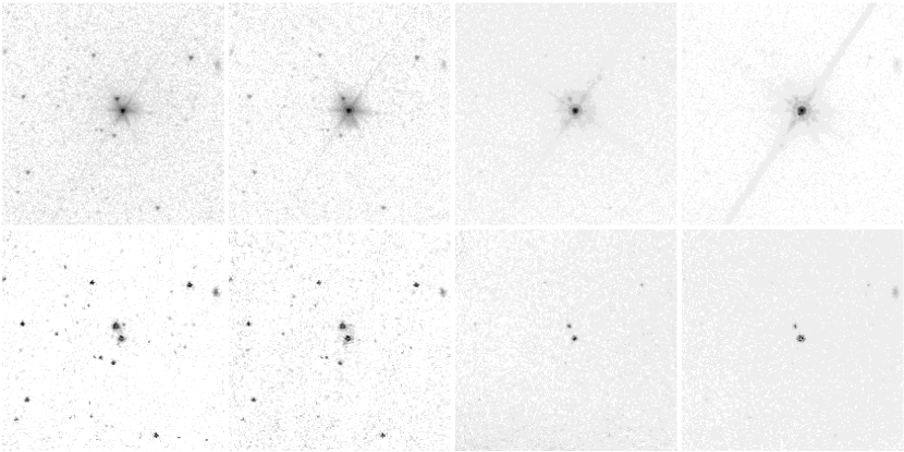
Figure 2.— Spitzer IRAC images at 3.6, 4.5, 5.8 and 8 $\mu$m during the bright state on 2005 July 17 (top four panels) and during the faint state on 2006 December 25 (bottom four panels). Only the central $8\times 8$ arcminutes of each image are shown (North up, East left). The transfer functions of each panel have been chosen individually to show the most detail.

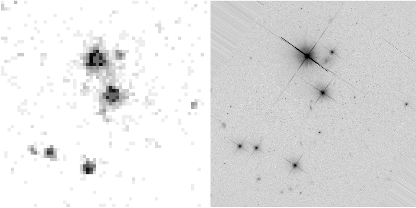
Figure 3.— Left: Spitzer IRAC image at 3.6 $\mu$m during the faint state on 2006 December 25. Right: Hubble image in the F814 filter (2004 August 4, provided by M. Chiaberge). Only the central $1.24\times 1.24$ arcminutes of each image are shown (North up, East left). The extension to the SE of 3C 454.3 in the IRAC image corresponds to two faint galaxies in the Hubble image.

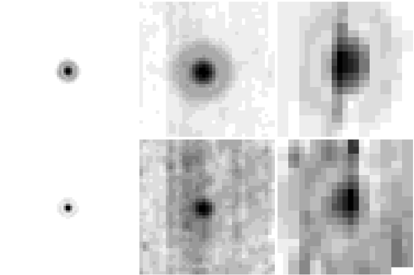
Figure 4.— Spitzer MIPS images at 24 $\mu$m (left), 70 $\mu$m (middle), and 160 $\mu$m (right) during the bright state on 2005 July 27 (top) and during the faint state on 2007 Jan 1 (bottom). Only the centers of each image are shown (in detector coordinates). The transfer functions of each panel have been chosen individually to bring out PSF details.

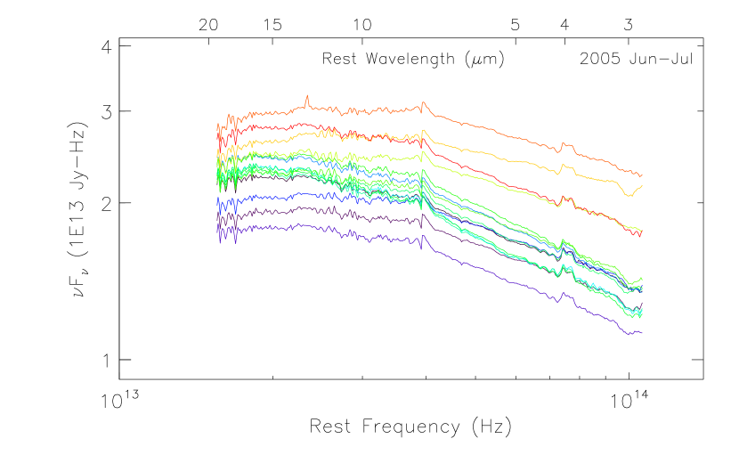
Figure 5.— Spitzer IRS low resolution spectra from 2005 June-July. The bumps at $4\times 10^{13}$ Hz and $7.3\times 10^{13}$ Hz (14 $\mu$m and 7 $\mu$m, observed) and the dip at $1\times 10^{14}$ Hz ($\sim 5.5$ $\mu$m, observed) are instrumental features. The noise spike at $2.2\times 10^{13}$ Hz (top spectrum) is an artifact of saturation. Other small bumps and wiggles in the spectra are attributable to residual detector fringes.

Figure 6.— Top: Spitzer IRS low resolution spectrum from 2006 December 20 low state. Bottom: Spectrum divided by best fit powerlaw ($\alpha=1.28$).

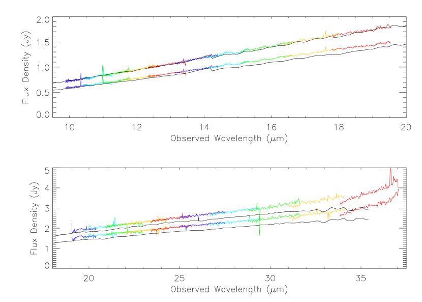
Figure 7.— High resolution spectra of 3C 454.3 (2005 epochs 1 and 15), with low resolution spectra (black lines) from the same epochs overlaid. Background has been subtracted for the low resolution spectra but not for the high resolution spectra (for which we had no separate background measurements), hence, there is an offset between the two spectra. Top panel: SH; bottom panel: LH.

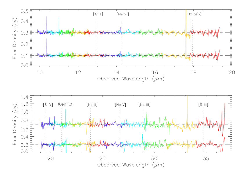
Figure 8.— Continuum-subtracted high resolution spectra of 3C 454.3. The 2005 epochs (1 and 15) are both offset from zero by an arbitrary amount for clarity. Top panel: SH; bottom panel: LH.

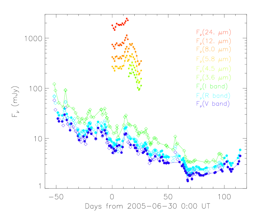
Figure 9.— Optical and mid-IR light curves for 2005 May-October. Optical V, R, and I band data from Foggy Bottom Observatory and Palomar Observatory are corrected for Galactic extinction and reddening. Mid-IR data are from the 2005 June 30-July 26 Spitzer IRS and IRAC campaigns. The optical fluxes showed flaring behavior superposed on an overall decline. Measurement uncertainties are generally smaller than the plot symbols.

Figure 10.— Spitzer IRS mid-IR light curves in three bands for 2005 Jun 30-July 14. Top: logarithmic scale; Middle: normalized in each band to the flux at epoch 3. The variability amplitude decreases with increasing wavelength at all times. Bottom: spectral index curves, solid line $=$ 6-24 $\mu$m index dotted line $=$ 6-12 $\mu$m index, and dashed line $=$ 12-24 $\mu$m index. The spectrum becomes harder during the bright flare that peaks on 2005 July 13, indicated with a vertical line.

Figure 11.— Color-flux diagram. The 6-24 $\mu$m spectral index is plotted vs. 6 $\mu$m flux. Triangles: 2005 June-July, square: 2006 December. During the 2005 epochs, there is a general trend for harder spectral index at greater flux. However, there is not a 1:1 correspondence, likely because the flux and spectral index depend on the detailed history of each IR flare.

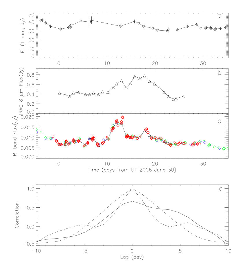
Figure 12.— Comparison of a) 1.3 mm (230 GHz) radio, b) IRAC 8.0 $\mu$m and c) R-band light curves. WEBT R-band data (Villata et al., 2006) are included with the Colgate and Palomar data to improve the sampling during the 2005 June-July Spitzer observation perod. The mm-wave variations do not appear to be correlated with the mid-IR variations, suggesting that emission in the two bands comes from separate regions in the jet. c) Cross-correlation of IRAC 8.0 $\mu$m and R-band light curves (solid line). The autocorrelation curves for IRAC 8.0 $\mu$m (dash), and R-band (dot-dash) are shown for comparison. The IR and optical emission are strongly correlated at zero lag.

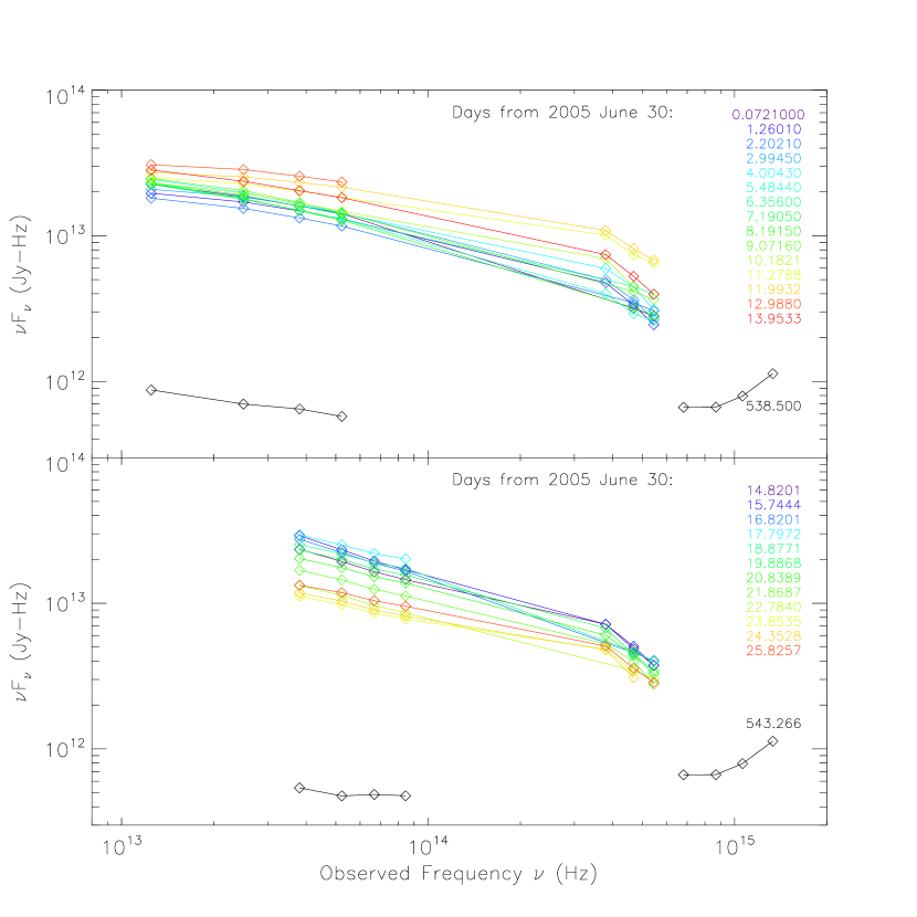
Figure 13.— SED time series in mid-to-near infrared and optical bands starting on 30 June 2005, and extending for 26 days, broken into two time periods including either the Spitzer IRS data or the Spitzer IRAC data, with dates distinguished in each frame by colors. Top: Optical-to-infrared (IRS) SED variability during 2005 June-July and on 2006 Dec 20. Bottom: Optical-to-infrared (IRAC) SED variability during 2005 June-July and on 2006 Dec 25. Most of the optical and near infrared measurements in 2005 June-July are from Palomar and Foggy Bottom Observatories; a few points are taken from WEBT data provided by M. Villata (Villata et al., 2007). For comparison, we show the rise in the SED (at $\sim 10^{15}$ Hz) attributed by Raiteri et al. (2008a) to the Big Blue Bump; B,U, W1, and M2 data points are from the Optical Monitor on XMM, taken on 2006 Dec 18-19, (Table 3 of Raiteri et al. (2007) ).

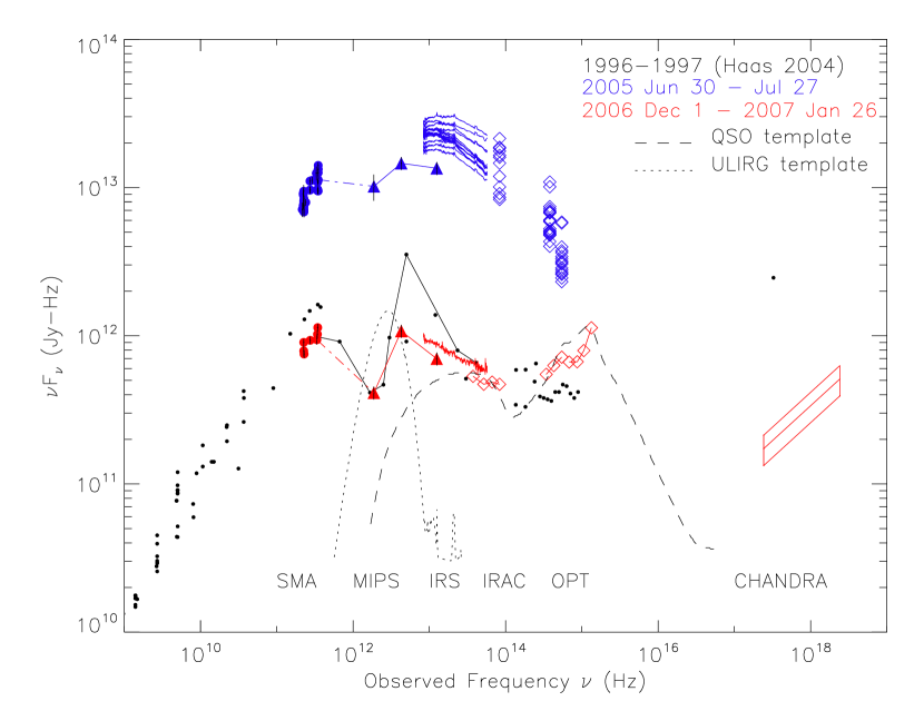
Figure 14.— 3C 454.3 SED. Spitzer MIPS 24, 70, and 160 $\mu$m photometry (triangles), IRS spectra (solid lines), and IRAC 3.6 $\mu$m and optical photometry (diamonds) are plotted together with other multiwavelength data. The mm and sub-mm points are SMA calibration data. Optical photometry in 2005 is from Foggy Bottom Observatory and the automated Palomar 1.5 m telescope. XMM-OM (UVM2, UVW1, U, B) photometry for 2006 Dec. 18-19 are from Raiteri et al. 2007, Table 3. V, R, and I photometry for 2006 Dec 20 are from WEBT data provided by M. Villata (Raiteri et al., 2007; Villata et al., 2007). Both sets have been corrected for extinction. Chandra X-ray data for the 2007 minimum are are indicated by the error box. The scattered small black dots are radio and optical photometry from the NED database, gathered from 1979-1995. The mean Richards et al. (2006) QSO SED (dashed line) and the Rieke et al. $10^{13}L_{\odot}$ ULIRG template (dotted line) are scaled and overplotted for comparison. Neither of these SEDs is compatible with the shape of the IR bump in the low-state 3C 454.3 SED, indicating a dominant nonthermal contribution from the jet. Note the presence of two synchrotron peaks, at IR and sub-mm wavelengths, in both the low and high states.

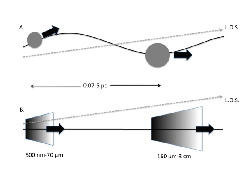
Figure 15.— A) Helical jet model. The two synchrotron peaks are produced by two relativistic blobs moving at different angles to the line of sight. The IR-optical peak is produced closer to the base of the jet, while the submm peak is produced further out. B) Inhomogeneous jet model. Two radially separated synchrotron emission regions give rise to the IR and submm synchrotron emission peaks. The IR emission region comes from the base of the jet, while the sub-mm emission region comes from a shock (possibly a jet recollimation shock) at a radius of $\sim 0.07-5$ pc. The direction to the observer’s line of sight is marked “L. O. S.”

References

- Abdo et al. (2009) Abdo, A. et al. 2009 ApJ, 699, 817
- Angione (1971) Angione R.J., 1971, AJ 76, 412
- Balonek (2005a) Balonek, T. 2005 vsnet-alert 8383
- Balonek (2005b) Balonek, T. 2005 vsnet-alert 8405
- Beckert (1989) Beckert, D. 1989, PASP, 101, 849
- Bottcher et al. (1997) Bottcher, M., Mause, H., & Schlickeiser, R. 1997, A&A, 324, 395
- Bonning et al. (2008) Bonning, E. W., Bailyn, C., Urry, C. M., Buxton, M., Fossati, G., Maraschi, L., Coppi, P., Scalzo, R., Isler, J., & Kaptur, A. 2009, ApJ 697, L81
- Cawthorne & Gabuzda (1996) Cawthorne, T. V., & Gabuzda, D. C. 1996, MNRAS, 278, 861
- Cenko et al. (2006) Cenko, S. B. et al. 2006, PASP, 118, 1396
- Ciaramella et al. (2004) Ciaramella, A. et al. 2004, A&A, 419, 485
- Cooper et al. (2007) Cooper, N. et al. 2007 ApJS 171, 376
- Craine (1977) Craine, E. R. 1977, “A handbook of quasistellar and BL Lacertae objects”, Astronomy and Astrophysics Series, Tucson: Pachart, 1977
- Decin & Eriksson (2007) Decin, L. & Eriksson, K. 2007, A&A, 472, 1041
- Decin et al. (2004) Decin, L., Morris, P. W., Appleton, P. N., Charmandaris, V., Armus, L., & Houck, J. R. 2004, ApJS, 154, 408
- Dickey & Lockman (1990) Dickey, J. M. & Lockman, F. J. ARA&A, 28, 215
- Donnarumma et al. (2009a) Donnarumma, I. et al. 2009, ApJ, 707, 1115
- Donnarumma et al. (2009b) Donnarumma, I., Vittorini, V., Vercellone, S., et al. 2009b, ApJ, 691, L13
- Fiorucci et al. (1998) Fiorucci M., Tosti G., Rizzi N., 1998, PASP 110,105
- Fossati et al. (1998) Fossati, Maraschi, L., Celotti, A. , Comastri, A., & Ghisellini, G.1998, MNRAS, 299, 433
- Fuhrmann et al. (2006) Fuhrmann, L. et al. 2006, A&A, 445, L1
- Ghisellini & Tavecchio (2009) Ghisellini, G. & Tavecchio, G. 2009, MNRAS, submitted, astro-ph 0902.0793
- Ghisellini et al. (1998) Ghisellini, G., Celotti, A., Fossati, G., Maraschi, L., & Comastri, A. 1998, MNRAS, 301, 451
- Giommi et al. (2006) Giommi, P. et al. A&A 456, 911
- Gomez, Marscher, & Albierdi (1999) Gomez, J.-L., Marscher, A. P., & Albierdi, A. 1999, ApJ, 577, 74
- Gordon et al. (2005) Gordon, K. D. et al. 2005 PASP 117, 503
- Gurwell et al. (2007) Gurwell, M.A., Peck, A.B., Hostler, S.R., Darrah,M.R., and Katz,C.A. (2007) ”Monitoring Phase Calibrators at Submillimeter Wavelengths”. From Z-Machines to ALMA: (Sub)Millimeter Spectroscopy of Galaxies ASP Conference Series, Vol. 375, proceedings of the conference held 12-14 January, 2006 at the North American ALMA Science Center, National Radio Astronomy Observatory, Charlottesville, Virginia, United States. Edited by Andrew J. Baker, Jason Glenn, Andrew I. Harris, Jeffrey G. Mangum and Min S. Yun., p.234
- Haas et al. (2004) Haas, M. et al. 2004, A&A, 424, 531
- Hagen-Thorn et al. (2009) Hagen-Thorn. et al. 2009, Astrophysical Reports, 53, 510
- Hartman et al. (1993) Hartman et al. 1993, ApJ, 407, L41
- Ho et al. (2004) Ho, P.T.P, Moran, J.M., and Lo, K.Y. 2004 ApJ, 616, L1
- Jorstad et al. (2001) Jorstad, S. G., Marscher, A. P., Mattox, J. R., Wehrle, A. E., Bloom, S. D., & Yurchenko, A. V. 2001, ApJS, 134, 181
- Kartaltepe & Balonek (2007) Kartaltepe & Balonek 2007, AJ, 133, 2866
- Kellerman et al. (2004) Kellerman, K. I. et al. 2004, ApJ, 609, 539
- Krolik (1999) Krolik, J. 1999, “Active Galactic Nuclei”, Princeton University Press: Princeton, NJ
- Lainela (1994) Lainela, M. 1994, A&A, 286, 408
- Levenson et al. (2007) Levenson, N. A., Sirocky, M. M., Hao, L., Spoon, H. W. @., Marshall, J. A., Elitzur, M., & Houck, J. R. 2007, ApJ, 654, L45
- Lind et al. (1989) Lind, K. R., Payne, D. G., Meier, D. L., & Blandford, R. D. 1989, ApJ, 344, 89
- Marscher et al. (2002) Marscher, A. P., Jorstad, S. G., Mattox, J. R., & Wehrle, A. E. 2002, ApJ, 577, 85
- Marscher & Gear (1985) Marscher, A. P. & Gear, W. K. 1985, ApJ, 298, 114
- McNaron-Brown et al. (1995) McNaron-Brown et al. 1995, ApJ, 451, 575
- Pauliny Toth et al. (1987) Pauliny-Toth, I. I. K., Porcas, R. W., Zensus, J. A., Kellerman, K. I., Wu, S. Y., Nicolson, G. D., & Mantovani F. 1987, Nature, 328, 778
- Pearson, Readhead, & Wilkinson (1980) Pearson, T. J., Readhead, A. C. S., & Wilkinson, P. N. 1980, ApJ, 2236, 714
- Pian et al. (2006) Pian, E. et al. 2006, A&A, 449, L21
- Pian, Falomo, & Treves (2005) Pian, E., Falomo, R., & Treves, A. 2005, MNRAS, 361, 919
- Raiteri et al. (2009) Raiteri, C. M. et al. 2009 A&A, 507, 769
- Raiteri et al. (2008a) Raiteri, C. M. et al. 2008, A&A, 491, 755
- Raiteri et al. (2008b) Raiteri, C. M. et al. 2008, A&A, 485, L17
- Raiteri et al. (2007) Raiteri, C. M. et al. 2007, A&A, 473, 819
- Raiteri et al. (1998) Raiteri C.M. et al., 1998, A and AS 130, 495
- Ravasio et al. (2003) Ravasio, M., Tagliaferri, G., Ghisellini, G. et al. 2003, A&A, 408, 479
- Reach et al. (2005) Reach, W. T., Megeath, S. T., Cohen, M., Hora, J., Carey, S., Surace, J., Willner, S. P., Barmby, P., Wilson, G., Glaccum, W., Lowrance, P., Marengo, M., & Fazio, G. F. 2005, PASP, 117, 978
- Richards et al. (2006) Richards, G. T. et al. 2006, ApJS, 166, 470
- Rieke et al. (2009) Rieke, G. H., Alonso-Herrero, A., Weiner, B. J., Perez-Gonzalez, P. G., Blaylock, M., Donley, J. L., & Marcillac, D. 2009, ApJ, 692, 556
- Savolainen et al. (2002) Savolainen, T., Wiik, K., Valtaoja, E., Jorstad, S. G. & Marscher, A. P. 2002, A&A 394, 851
- Scott et al. (2003) Scott, W. K. et al. 2004, ApJS, 155, 33
- Smith & Balonek (1998) Smith, P. S., & Balonek, T. J. 1998, PASP, 1110, 1164
- Smith et al. (1988) Smith, P. S., Elston, R., Berriman, G., Allen, R. G., & Balonek, T. J. 1988, ApJ, 326, L39
- Tavecchio et al. (2002) Tavecchio, F., Maraschi, L., Ghisellini, G., Celotti, A., Chiappetti, L., Comastri, A., Fossatti, G., Grandi, P., Pian, E., Tagliaferri, G., Treves, A., & Sambruna, R. 2002, ApJ, 575, 137
- Vercellone et al. (2009a) Vercellone, S. et al. 2009, ApJ, 690, 1018
- Vercellone et al. (2009b) Vercellone, S. et al. 2009, astro-ph 0910.5325, to appear in ”Accretion and Ejection in AGN: A Global View”, ASP Conf. Series, ed. L. Maraschi, G. Ghisellini, R. Della Ceca, and F. Tavecchio.
- Vercellone et al. (2008) Vercellone, S. et al. 2008, ApJ, 676, L13
- Villata et al. (2009) Villata, M. et al. 2009, A&A, 504, L9
- Villata et al. (2007) Villata, M. et al. 2007, A&A, 464, L5
- Villata et al. (2006) Villata, M. et al. 2006, A&A, 453, 817
- Villata & Raiteri (1999) Villata, M. & Raiteri, C. M. 1999, A&A, 347, 30
- Wehrle et al. (1998) Wehrle, A. E. et al. 1998, ApJ, 497, 178
- Zhang et al. (2005) Zhang, S., Collmar, W., & Schonfelder, V. 2005, A&A, 444, 767