Magnetic field detection in the B2 Vn star HR 7355

Abstract

The B2Vn star HR 7355 is found to be a He-rich magnetic star. Spectropolarimetric data were obtained with FORS1 at UT2 on Paranal observatory to measure the disk-averaged longitudinal magnetic field at various phases of the presumed 0.52 d cycle. A variable magnetic field with strengths between $\langle B_{z}\rangle=-2200$ and $+3200$ G was found, with confidence limits of 100 to 130 G. The field topology is that of an oblique dipole, while the star itself is seen about equator-on. In the intensity spectra the Hei-lines show the typical equivalent width variability of He-strong stars, usually attributed to surface abundance spots. The amplitudes of the equivalent width variability of the Hei lines are extraordinarily strong compared to other cases. These results not only put HR 7355 unambiguously among the early-type magnetic stars, but confirm its outstanding nature: With $v\sin i=320$ km s^-1 the parameter space in which He-strong stars are known to exist has doubled in terms of rotational velocity.

1 Introduction

Rivinius et al. (2008) suggested the B2Vn star HR 7355 (HD 182 180, HIP 95 408) to be a He-rich magnetic star with a magnetosphere containing trapped gas that produces hydrogen line emission (Townsend & Owocki 2005, Townsend, Owocki & Ud-Doula 2007). They based their suggestion on evidence derived from two FEROS echelle spectra and a Hipparcos light-curve, with a period of either single-wave 0.26 d or double-wave 0.52 d. However, a period of 0.26  could not be due to rotational modulation, since this would require a rotational speed well above the critical threshold.

If confirmed, HR 7355 would have a unique position in the He-strong class: With $v\sin i=320$ km s^-1 (Abt, Levato & Grosso 2002) it would be the the most rapidly rotating magnetic star in the upper HR-diagram; by a factor of about two ahead of the current record-holder, $\sigma$ Ori E, which has $v\sin i=165$ km s^-1 (Abt et al., op. cit.). This would make the star a show-case for the Rigidly Rotating Magnetosphere model, that so far, though with great success, was applied to only one star, $\sigma$ Ori E (Townsend & Owocki, op. cit.). In order to test this claim, a spectropolarimetric campaign was carried out in 2008.

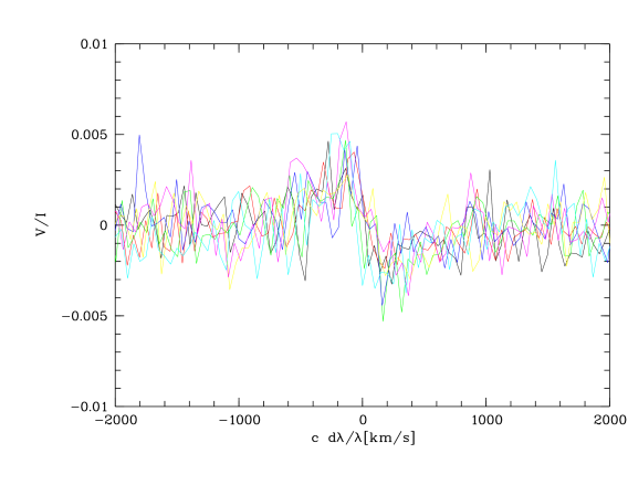
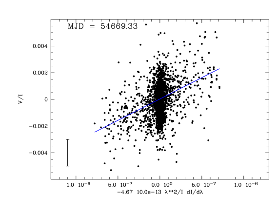
Figure 1: Normalized circular polarization $V/I$ of HR 7355 at MJD=54669.33, for which a longitudinal magnetic field component of 3200 G was derived. Top: The spectra around the ten Balmer lines from H$\beta$ to H₁₃. Bottom: The $V/I$ vs. the bracketed part of the right term in Eqn. 1 and the linear regression to the data as a solid line. The typical error per measurement is shown as a bar; the error in the abscissa is less than the symbol size. The mass of points clustering around (0,0) are due to the unpolarized continuum.

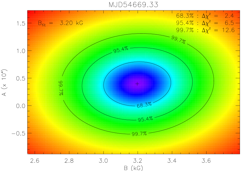
Figure 2: Minimum of the two-dimensional probability density disctribution computed from the artificial test data (see Sect. 3.1) for the observed data shown in Fig. 1, and an overplot of the $\chi^{2}$-contrours enclosing 68.3%, 95.4% and 99.7% probabilities (upper panel) and one dimensional probability distribution of the derived field strength (lower panel).

2 Observations and Data Reduction

The data described below were obtained at the VLT with the FORS1 instrument (Appenzeller et al. 1998), which is equipped with a super-achromatic quarter-wave retarder plate. The instrument setup used the 1200B holographic prism with a dispersion of 24 Å/mm over a range of 366 to 511 nm. At a slit-width of 0.3″, a (binned) pixel scale of 0.25″per pixel, and a (binned) pixel size of 30 $\mu$m, this gives about 0.9 Å per pixel, which slightly oversamples the resolution element of about 1.3 Å.

Each individual measurement (see Table 1) consisted of a sequence of eight exposures, taken at retarder plate position angles in the sequence ($-45\degr,-45\degr,45\degr,45\degr,-45\degr,-45\degr,45\degr,45\degr$) with respect to the axis of the Wollaston prism. The exposure time was two seconds for the respective 8 exposures. The data was taken during four nights in service mode. During two of these nights the sequence was repeated, so that we have obtained six data sets, each one reaching an approximate S$/N$-ratio of about 1000 per resolution element. The method for extracting the Stokes $V$ parameter from the data is described in the FORS user manual (Jehin & O’Brien 2008) and by Bagnulo et al. (2002).

Example Stokes V data are presented in Fig. 1; in this figure, and for the field strength determination (as in Fig. 2), there is no rebinning from pixel space to uniform wavelength space. We calculated the wavelength for the respective data points based on the HgCd and He arc line spectra taken during daytime.

Flat fielding is largely unnecessary for the Stokes $V$ determinations, because the alternate measurement of $-V/I$ and $V/I$ at $-45\degr$ and $45\degr$ retarder plate angles cancels out any pixel-to-pixel variations in the CCD response; nevertheless, because intensity ($I$) data are required to derive the field strength, we applied an appropriate flat-field correction to all spectra.

MJD	$\langle B_{z}\rangle$	$\sigma_{B_{z}}$	$W_{\lambda,{\rm He}{\rm I}\,4388}$	$W_{\lambda,{\rm He}{\rm I}\,4713}$	phase
	[G]	[G]	[mÅ]	[mÅ]
54652.327	-2210	$\pm$ 130	1720	530	0.681
54656.078	-1760	$\pm$ 130	850	310	0.875
54656.146	230	$\pm$ 100	740	280	0.006
54661.327	-1110	$\pm$ 120	660	250	0.942
54669.186	220	$\pm$ 110	820	310	0.013
54669.330	3200	$\pm$ 130	1530	480	0.289

Table 1: List of magnetic field and equivalent width measurements derived from the FORS1 data. The typical error for the equivalent width is about 5 %. For computing the phase we use the ephemeris defined in Eqn. 3. Only Balmer lines were included in the field measurements.

3 Results

3.1 Magnetic field

As discussed by Bagnulo et al. (2002), under the weak field approximation one can derive the mean longitudinal magnetic field component over the stellar disk $\langle B_{z}\rangle$ from the circular polarimetry and the gradient of the intensity spectrum with the equation:

$$\frac{V}{I}=\left[-{\rm g}_{\rm eff}{\rm C}_{z}\lambda^{2}\frac{{\rm d}I}{I~{}\rm{d}\lambda}\right]\times\langle B_{z}\rangle$$ (1)

Here we used a factor ${\rm C}_{z}$ summarizing the physical constants like the electron charge ${\rm e}$, the electron mass ${\rm m_{e}}$ and the speed of the light ${\rm c}$ in the form:

$${\mathrm{C}}_{z}=\frac{\mathrm{e}}{4\pi{\mathrm{m}}_{\mathrm{e}}{\mathrm{c}}^{2}}\sim 4.67\,10^{-13}\mbox{\rm\AA}^{-1}\mbox{\rm G}^{-1}$$ (2)

and an effective Landé factor ${\rm g}_{\rm eff}=1$ as discussed by Casini & Landi Degl’Innocenti (1994).

It should be clearly mentioned that there are a number of approximations and assumptions in equation 1 above. One of those is the week field approximation for the magnetism, i.e. a Zeeman split of less then the intrinsic line thermal and pressure broadening, which is, however, safely applicable to a field of only a few kilogauss in a main sequence B star. A concern prompting far more caution when interpreting the derived numbers is that the spectra are, in fact, an average over the stellar disk longitudinal field component, without considering e.g. the limb darkening (See Bagnulo et al. 2002, for a full discussion of the limitations and caveats of the method). However, as this quantity, labelled $\langle B_{z}\rangle$, is typially the most easily derived magnetic observable, it is also the most published in the literature (Wade 2003), and as such easily comparable to other measurements. A more complete magnetic modelling to derive the physical dipole field strength is left to a later work.

We used a $\chi^{2}$ minimization approach to fit the linear model $V/I=A+\langle B_{z}\rangle\times x$ to the observational data; this model is based on eqn. 1 with the addition of a constant term $A$. The additional term $A$ is physically expected to be zero, as it is the $V/I$ of the continuum. However, the employed measurement principle does not necessarily guarantee $A=0$ in the measured data, so we allow non-zero values in order to improve the linear regression to the slope. It actually turns out that the derived values for $A$ are consistently above zero by between $0.4\times 10^{-4}$ and $2.5\times 10^{-4}$ with a typical $\sigma=0.5\times 10^{-4}$, and on average $1.5\times 10^{-4}$. This likely is an instrumental effect. In any case this is rather small compared to the $V/I$ peak-to-peak amplitude induced by the magnetic field, which is up to 40 times higher (see Fig. 1)..

The formal errors of $V/I$, which are derived from the well known photon- and detector noise characteristics, were used to assign weights for the $\chi^{2}$ fit. The derived $\langle B_{z}\rangle$ are given in Table 1.

Given recent concerns expressed over the error bars associated with FORS1 magnetic field measurements (see, e.g. Silvester et al. 2009), we have exercised particular care in deriving the errors listed in Table 1. Applying the bootstrap Monte Carlo approach described by Press et al. (1992), we used the observational data from each epoch to construct one million corresponding synthetic datasets. We then applied the same fitting approach as above to obtain $A$ and $\langle B_{z}\rangle$ values for every synthetic dataset. These values exhibit a distribution about those derived from the actual observations; Fig. 2 shows this distribution for the MJD 54 669.330 observations, both as a 2-dimensional probability density map, and as a 1-dimensional probability density function in $\langle B_{z}\rangle$. Plotted over the map are contours of constant $\chi^{2}$ that enclose 68.3%, 95.4% and 99.7% of the synthetic datasets; likewise, plotted over the probability density function are the symmetric bounds enclosing 68.3%, 95.4% and 99.7% of the synthetic datasets. The bounds for the 68.3% case are assigned as the error bars quoted in Table 1; because the probability density function in Fig. 2 is close to Gaussian (and likewise for the data from other epochs), these error bars can be regarded as approximate 1-$\sigma$ confidence intervals. Note, however, that we have not made any specific assumptions regarding the propagation of errors through our modeling process; the Monte Carlo approach naturally results in error estimates that directly reflect the combined characteristics of the observations and the modeling.

3.2 Spectral lines

Next to the Stokes $V$ spectra, we examined the intensity spectra observed by FORS1. Due to the very high $S/N$ and the large rotational velocity, even the relatively low dispersion of FORS1 allows high quality equivalent width (EW) measurements of the spectral lines.

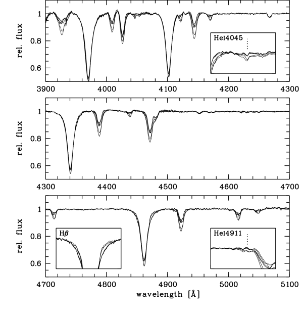
Figure 3: Intensity spectra measured by FORS. The Hei-variability is well seen, while the Balmer lines vary only little and the Cii 4267 and Siiii 4552 lines remain stable.

The Hi lines, with the exception of H$\beta$, show little variability, except in the very core. The spectra taken at MJD=54656.146 and 54669.186 show enhanced core absorption. At these epochs the $\langle B_{z}\rangle$ had null-detections, which is in agreement with the crossing of the magnetic equator through the line of sight, because this is the time at which a corotating cloud of circumstellar matter, located at the crossing of the magnetic and rotational equators, is expected to pass in front of the star.

In H$\beta$ this circumstellar absorption is seen as well, but in addition the other four spectra show variability in the line wings, in particular in the red one. This is probably a signature of the circumstellar emission arising in the corotating clouds, well seen in the two FEROS spectra (Rivinius et al. 2008) for H$\alpha$.

All Hei lines in the observed range follow a similar variation pattern, varying both in strength and in profile. The lines showing strong broadening wings have a larger amplitude in $W_{\lambda}$ due to variation in these wings, but the profile variability is better seen in weaker lines, like Hei 4713.

3.3 Forbidden Hei lines

In addition to the well known stellar Hi and Hei lines, there is significant variability at $\lambda\approx 4045$ Å and bluewards of Hei4922, at $\lambda\approx 4911$ Å. We identify the features with the forbidden lines Hei4045 ($2^{3}P\rightarrow 5^{3}P$) and Hei4911 ($2^{1}P\rightarrow 4^{1}P$), features well known in extreme Helium stars (Beauchamp & Wesemael 1998).

In the FORS data, variability due to forbidden components of Hei at $\lambda\lambda$ 4045 and 4911 was found. At a closer inspection, this spectral signature is also present in the old FEROS spectra, and a search in other magnetic He-strong stars reveals the presence of these lines also in $\sigma$ Ori E and V 1046 Ori. Less certain, though not excluded from our archival data, are those lines in HD 64 740 and HD 37 776 (Fig. 5). These lines are never seen in B stars with normal He abundance.

In other words, the presence of these lines indicates a Helium overabundance wrt. solar values. Such He-strong stars, especially when having rotationally broadened lines, are quite hard to diagnose without detailed abundance analysis, as has also happened for HR7355, instead of classifying it as chemically peculiar it was rather classified as a later type that it actually has. This means the presence of the two forbidden Helium lines can safely be taken as an indicator for a He-strong star. As many He-strong stars are magnetic (and He-weak stars are typically of later spectral type), with the same reasoning we consider the presence of these lines as an indicator for a magnetic field in early B-type stars.

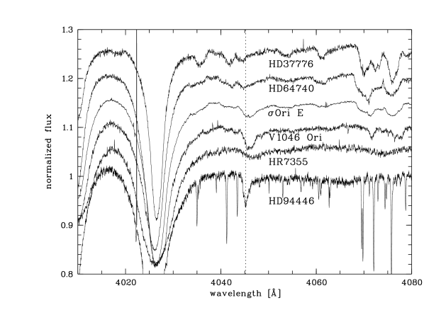
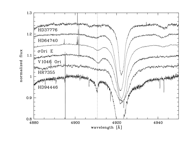
Figure 4: Forbidden Hei 4045,4911 signatures in some known magnetic He-strong stars. The forbidden components are clearly seen in in the slowly rotating HD 94 446, but also in HR 7355, V1046 Ori and $\sigma$ Ori E, and possibly in HD 64 740 and HD 37 776 as well. Note that these are single spectra, so shifts occur as the features are Doppler shifted due to the rotational variation.

4 Discussion

4.1 Ephemeris

As we know from $\sigma$ Ori E (Reiners et al. 2000), the phase most easy to pin down, both spectroscopically and photometrically, is the center of one of the two circumstellar clouds crossing in front of the star. We chose this point also for HR 7355 as $\phi=0$. A corresponding epoch $T_{0}$ can then be identified as the time of strongest absorption in H$\alpha$, i.e. the maximal equivalent width. While our FORS data do not cover H$\alpha$, and the FEROS data were not taken in this phase, a spectroscopic campaign with the echelle instrument UVES at Paranal that has been completed in the second half of 2009, suggests MJD$=54\,940.33$ as epoch. However, since a full analysis of the UVES data is far beyond the scope of this discovery report, and the epoch is not as critical as the period for our purpose, we leave a detailed analysis and discussion of the H$\alpha$ equivalent width curve to a later work (Rivinius et al, in prep.), and here just adopt the epoch. Nevertheless it is reassuring that additional absorption in H$\beta$ in the FORS1 data is observed at $\phi=0.006$ and $0.013$, when the data are sorted with the period derived below. These two occurrences, 25 cycles apart from each other and more than 500 cycles apart from the selected epoch, are in full agreement with this epoch derived from UVES data.

For the period, Rivinius et al. (2008) gave a value of 0.521428(6) d for the Hipparcos data, under the condition that the variations were double-wave sinsoidal. The single wave period, which in any case would have been to short to be rotational, is firmly excluded by the new magnetic measurements.

However, also the 0.52 d period is not able to satisfactorily phase all available data, and so its value had to be improved. In order to do so, we demand a period to sort all three data types, i.e. the photometric data (1990-1993, double wave), the magnetic data (2008, single wave), and the equivalent widths (1999-2008, possibly double wave). With respect to the originally published value, the closest period soring all three data-types is $0.521442(4)$ d. Although the EW data suffers strong seasonal aliasing, already its most nearby alias is excluded by the almost completely scrambled photometric curve for this period. The most nearby period value for which EW and photometry could be reconciled is incompatible with the magnetic phase-curve. We thus conclude that the true rotational period of HR 7355 must be within the above value’s uncertainties.

In a final step, we can assume that the photometric minima do have a certain phase relation to the spectroscopic curve. There are two possiblities: First, the minima could be due to cloud eclipses in front of the star, then we can further require that one of the photometric minima occurs at phase $\phi=0$. Second, the photometric might be due to photospheric flux modulation in the He-enriched parts (Krtička et al. 2007; Mikulášek et al. 2010). In this case, the photometric minima would coincide with minimal Hei equivalent width. However, in this particular star, the maximal $H\alpha$ equivalent width and the minimal Hei equivalent width are almost simultaneous, so that a final decision about this can only be made with new photometry more simultanous with recent observations. in any case, already with the period derived from the equivalent widths alone one of the two photometric minima is very close to $\phi=0$, so that under the assumption that the photometric variability is due to the circumstellar material obscuring the line of sight the period becomes $P=0.521444(3)$ d. We will use the latter value for the discussion, but note that this relies on the assumption that the photometric minima are due to eclipses, while the best period without this assumption is $P=0.521442(4)$ d

The ephemeris used thus is

$$T_{\rm{H}{\rm I}~{}max.~{}absorption}({\rm MJD})=54940.33+0.521444(3)\times E$$ (3)

4.2 Periodic variations

With the above choice of epoch we expect to see photometric minima, as well as $B_{z}=0$, at phase $\phi=0$, i.e. when the magnetic equator is facing towards us (Fig. 5). Then using the above ephemeris, and assuming a sinusoidal variation of the magnetic field, we estimate the field curve as

$$\langle B_{z}\rangle(t)=350\,{\rm G}+2850\,{\rm G}\times\sin\left(2\pi\left(\frac{t\rm-T_{0}}{P}-0.02\right)\right)$$ (4)

where $t$ is the date, and $T_{0}$ and $P$ are epoch and period from Eqn. 3, and the shift of 0.02 in phase is required to fulfill the above condition $B_{z,\phi=0}=0\,$G, due to the constant term of 350 G.

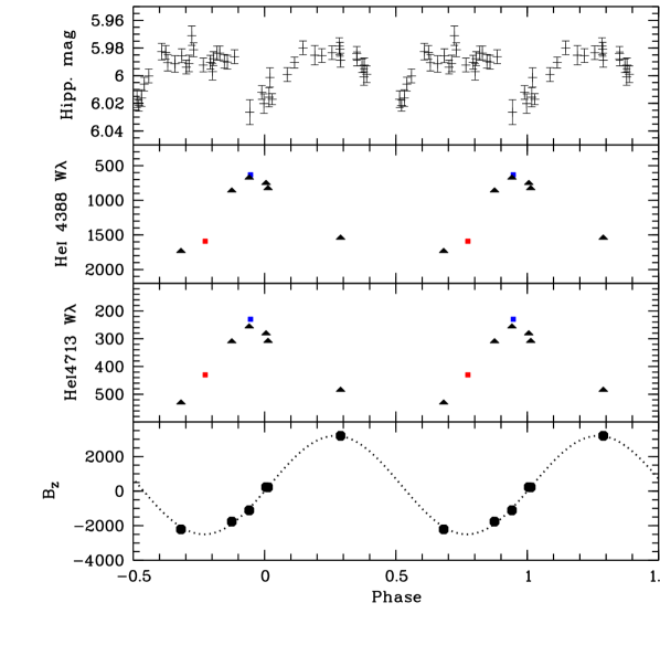
Figure 5: Measured quantities (see Table 1, also for typical errors) as function of the rotational phase (Eqn 3). The Hipparcos double wave light-curve is shown in the uppermost panel, the Hei 4388 and 4713 equivalent widths below as triangles. The $W_{\lambda}$ measured in the FEROS spectra (Rivinius et al. 2008) are shown as red (1999 data) and blue (2004 data) squares. The lowermost panels shows the $\langle B_{z}\rangle$ field measurements and the curve defined by Eqn. 4.

The fact that $B_{\rm max}\approx-B_{\rm min}$ confirms the assumption of $i\approx 90^{\circ}$ by Rivinius et al. (2008), while the term of 350 G is easily explained either by a slight offset from this value, or by an off-center magnetic dipole.

Such an off-center dipole would cause a non-sinusoidal field curve. In fact, due to two datapoints being taken at identical phases, there are effectively only five points to constrain the three free parameters of Eqn. 4. The field curve, although it seems to fit very well, is thus not well constrained, which is why we cannot really give confidence limits for the parameters unless further data has been obtained. In particular, we stress that the exactly sinusoidal shape of the curve is rather an assumption than an actually observed property.

When the magnetic poles face the observer, $\langle B_{z}\rangle$ becomes maximal. Although there are only few points, not sampling the curve in all detail and in particualr not necessarily the respective maxima and minima, it is clear that the Hei absorption is much stronger in these phases than when the magnetic equator is visible (Fig. 5). This is in full agreement with the behavior observed in other He-strong stars, like $\sigma$ Ori E (Reiners et al. 2000).

The amplitude of the Hei EW variations is considerably larger than in $\sigma$ Ori E, however. There the maximal EW is only about a factor of 1.3 to 1.5 stronger than the minimal one, depending on the spectral line. In HR 7355 the lines strengthen, wrt. their minima, by a factor of 2 for lines like Hei4713, and even a factor of 3 for strong lines with significant broadening wings like Hei4388. This strong modulation is indicative for two large Helium enhanced patches on the surface close the equator at opposite longitudes, which point to a large angle $\beta$ between the rotational and magnetic axes.

5 Summary

The results confirm the magnetic and He-strong nature of HR 7355. We have detected a magnetic field of multi-kilogauss strength, varying with the rotational period, which is $P=0.521444(3)$ d under the assumption of the photometric minima being eclipses, and $P=0.521442(4)$ d without this assumption. In order to avoid a potential underestimation of the confidence limits of the magnetic field measurement (as suspected for previous FORS measurements by Silvester et al. 2009), we derived them with a boot-strap Monte-Carlo method, which does not implicitely assume a statistics for the error propagation, but numerically reconstructs the probability distribution from which the actual observation was drawn.

The observed magnetic field and the suggested topology (see Sect. 4.2) is in agreement with the initial hypothesis by Rivinius et al. (2008), namely that of an equatorially seen star, i.e. $i\approx 90^{\circ}$, with an oblique magnetic dipole. This topology gives rise to a double-wave light curve, either as the corotating magnetospheric clouds, magnetically bound at the crossings of magnetic and rotational equator, sweep through the line of sight twice per rotational period (Townsend 2008), or due to the modulation of the photospheric flux by the abundance pattern (Mikulášek et al. 2010).

References

- Abt et al. (2002) Abt H. A., Levato H., Grosso M., 2002, ApJ, 573, 359
- Appenzeller et al. (1998) Appenzeller I., Fricke K., Fürtig W., Gässler W., Häfner R., et al 1998, The Messenger, 94, 1
- Bagnulo et al. (2002) Bagnulo S., Szeifert T., Wade G. A., Landstreet J. D., Mathys G., 2002, A&A, 389, 191
- Beauchamp & Wesemael (1998) Beauchamp A., Wesemael F., 1998, ApJ, 496, 395
- Casini & Landi Degl’Innocenti (1994) Casini R., Landi Degl’Innocenti E., 1994, A&A, 291, 668
- Jehin & O’Brien (2008) Jehin E., O’Brien K., 2008, FORS user manual (VLT-MAN-ESO-13100-1543). ESO, period 81 edn
- Krtička et al. (2007) Krtička J., Mikulášek Z., Zverko J., Žižńovský J., 2007, A&A, 470, 1089
- Mikulášek et al. (2010) Mikulášek Z., Krtička J., Henry G. W., de Villiers S. N., Paunzen E., Zejda M., 2010, A&A, 511, L7
- Press et al. (1992) Press W. H., Teukolsky S. A., Vetterling W. T., Flannery B. P., 1992, Numerical recipes in FORTRAN. The art of scientific computing. Cambridge: University Press
- Reiners et al. (2000) Reiners A., Stahl O., Wolf B., Kaufer A., Rivinius T., 2000, A&A, 363, 585
- Rivinius et al. (2008) Rivinius T., Štefl S., Townsend R. H. D., Baade D., 2008, A&A, 482, 255
- Silvester et al. (2009) Silvester J., Neiner C., Henrichs H. F., Wade G. A., Petit V., et al 2009, MNRAS, 398, 1505
- Townsend (2008) Townsend R. H. D., 2008, MNRAS, 389, 559
- Townsend & Owocki (2005) Townsend R. H. D., Owocki S. P., 2005, MNRAS, 357, 251
- Townsend et al. (2007) Townsend R. H. D., Owocki S. P., Ud-Doula A., 2007, MNRAS, 382, 139
- Wade (2003) Wade G. A., 2003, in L. A. Balona, H. F. Henrichs, & R. Medupe ed., Astronomical Society of the Pacific Conference Series Vol. 305 of Astronomical Society of the Pacific Conference Series, Measuring the Characteristics of Magnetic Fields in A, B and O Stars. p. 16