Shear Dynamics in Bianchi I Cosmology

Abstract:

We present the exact equation for evolution of Bianchi I cosmological model, considering a non-tilted perfect fluid in a matter dominated universe. We use the definition of shear tensor and later we prove it is consistent with the evolution equation for shear tensor obtained from Ricci identities and widely known in literature [3], [5], [9]. Our result is compared with the equation given by Ellis and van Elst in [3] and Tsagas, Challinor and Maartens [5]. We consider that it is important to clarify the notation used in [3], [5] related with the covariant derivative and the behavior of the shear tensor.

1 1+3 Orthonormal frame approach

In a cosmological space-time $(\mathcal{M},\mathbf{g})$ there are preferred worldlines representing the average motion of matter at each point, associated with comoving or fundamental observers, which do not have peculiar velocities. The signature used in this article is $(-+++)$. The 4-velocity of the comoving particles is $u^{\alpha}$, $u^{\alpha}=(1,0,0,0)$, $u^{\alpha}u_{\alpha}=-1$. This 4-velocity is orthogonal to the surfaces of spatial homogeneity. Therefore, it is defined the spatial projection tensor $h_{\alpha\beta}$ as [3], [10]:

$$h_{\alpha\beta}:=g_{\alpha\beta}+u_{\alpha}u_{\beta},$$ (1)

given this tensor, we can define the orthogonally projected symmetric trace-free part of any tensor $T^{\alpha\beta}$ of second rank as:

$$T^{\langle\alpha\beta\rangle}=\left[h^{(\alpha}_{\ \ \gamma}h^{\beta)}_{\ \ \delta}-\frac{1}{3}h^{\alpha\beta}h_{\gamma\delta}\right]T^{\gamma\delta},$$ (2)

moreover, other two derivatives can be defined [3]: the covariant time derivative, along the fundamental worldlines, where for any tensor $T^{\alpha\beta}_{\ \ \gamma\delta}$:

$$\dot{T}^{\alpha\beta}_{\ \ \gamma\delta}:=u^{\epsilon}\nabla_{\epsilon}T^{\alpha\beta}_{\ \ \gamma\delta},$$ (3)

and the fully orthogonally projected covariant derivative $\tilde{\nabla}$, where:

$$\tilde{\nabla}_{\epsilon}T^{\alpha\beta}_{\ \ \gamma\delta}=h^{\alpha}_{\ \mu}h^{\beta}_{\ \nu}h^{\kappa}_{\ \gamma}h^{\lambda}_{\ \delta}h^{\eta}_{\ \epsilon}\nabla_{\eta}T^{\mu\nu}_{\ \ \kappa\lambda}.$$ (4)

Given these derivatives, the 4-aceleration can be written as $\dot{u}_{\alpha}=u_{\alpha;\beta}u^{\beta}$. With these definitions the first covariant derivative of $u_{\alpha}$ is decomposed into its irreducible parts, defined by their symmetry properties [3], [10]:

$$\nabla_{\beta}u_{\alpha}=-\dot{u}_{\alpha}u_{\beta}+\omega_{\alpha\beta}+\sigma_{\alpha\beta}+\frac{1}{3}\Theta h_{\alpha\beta},$$ (5)

where $\sigma_{\alpha\beta}:=u_{(\alpha;\beta)}-\dot{u}_{(\alpha}u_{\beta)}-\frac{1}{3}\Theta h_{\alpha\beta}$ is the trace-free symmetric rate of shear tensor $(\sigma_{\alpha\beta}=\sigma_{(\alpha\beta)},\ \sigma_{\alpha\beta}u^{\beta}=0,\ \sigma^{\alpha}_{\ \alpha}=0)$, which describes the rate of distortion of the matter flow; and $\omega_{\alpha\beta}:=u_{[\alpha;\beta]}-\dot{u}_{[\alpha}u_{\beta]}$ is the skew-symmetric vorticity tensor $(\omega_{\alpha\beta}=\omega_{[\alpha\beta]},\ \omega_{\alpha\beta}u^{\beta}=0)$, describing the rotation of the matter relative to a non-rotating (Fermi-propagated) frame [3].

It is possible to obtain a propagation equation for the shear tensor, from Ricci identities [3], [5]:

$$\dot{\sigma}^{\langle\alpha\beta\rangle}-u^{\langle\alpha}u^{\beta\rangle}=-\frac{2}{3}\Theta\sigma^{\alpha\beta}+\dot{u}^{\langle\alpha}\dot{u}^{\beta\rangle}-\sigma^{\langle\alpha}_{\gamma}\sigma^{\beta\rangle\gamma}-\omega^{\langle\alpha}\omega^{\beta\rangle}-\left(E^{\alpha\beta}-\frac{1}{2}\pi^{\alpha\beta}\right),$$ (6)

where $E^{\alpha\beta}$ is the Electric Weyl tensor, $E_{\alpha\beta}=C_{\alpha\gamma\beta\delta}u^{\gamma}u^{\delta}$, where $C_{\alpha\beta\gamma\delta}$ is the Weyl tensor, and $\pi_{\alpha\beta}=T_{\gamma\delta}h^{\gamma}_{\ \langle\alpha}h^{\delta}_{\ \beta\rangle}$, where $T_{\alpha\beta}$ is the energy momentum tensor and $\pi_{\alpha\beta}$ is the trace-free anisotropic pressure.

The Weyl Tensor is completely determined from its electric and magnetic parts, the last one defined as [3], [4] defined as:

$$H_{\alpha\beta}=\frac{1}{2}\eta_{\alpha\delta\epsilon}C^{\delta\epsilon}_{\ \ \beta\gamma}u^{\gamma},$$ (7)

where $\eta_{\alpha\beta\gamma}=u^{\delta}\eta_{\delta\alpha\beta\gamma}$ is a volume element for the rest spaces and $\eta_{\alpha\beta\gamma\delta}$ is the 4-dimensional volume element [3] $(\eta_{\alpha\beta\gamma\delta}=\eta_{[\alpha\beta\gamma\delta]},\ \eta_{0123}=\sqrt{|\det(g_{\alpha\beta})|})$.

Using the Gauss-Codacci relation the Spatial Riemann Tensor is [5]:

$${}^{3}R_{\alpha\beta\gamma\delta}=h^{\zeta}_{\ \alpha}h^{\eta}_{\ \beta}h^{\theta}_{\ \gamma}h^{\vartheta}_{\ \delta}R_{\zeta\eta\theta\vartheta}-\tilde{\nabla}_{\gamma}u_{\alpha}\tilde{\nabla}_{\delta}u_{\beta}+\tilde{\nabla}_{\delta}u_{\alpha}\tilde{\nabla}_{\gamma}u_{\beta}.$$ (8)

and the Spatial Ricci tensor is:

$$^{3}R_{\alpha\beta}=-\dot{\sigma}_{\langle\alpha\beta\rangle}-\Theta\sigma_{\alpha\beta}+\tilde{\nabla}_{\langle\alpha}\dot{u}_{\beta\rangle}+\dot{u}_{\langle\alpha}\dot{u}_{\beta\rangle}+\pi_{\alpha\beta}+\frac{1}{3}h_{\alpha\beta}\left[2\mu-\frac{2}{3}\Theta^{2}+2\sigma^{2}+2\Lambda\right],$$ (9)

where $\mu$ is the energy density and $\sigma^{2}=\frac{1}{2}\sigma^{\alpha\beta}\sigma_{\alpha\beta}$.

2 Bianchi I cosmology

Bianchi cosmologies are spatially homogeneous but not necessarily isotropic. For a review of Bianchi models, see [1], [2], [9] and for orthonormal frame approach [3], [4], [9].

Here we will consider Bianchi I cosmology. The metric of this model is given by [4], [5], [6], [7]:

$$ds^{2}=-dt^{2}+a^{2}(t)dx^{2}+b^{2}(t)dy^{2}+c^{2}(t)dz^{2},$$ (10)

and the average expansion scale factor $S(t)=\sqrt[3]{abc}$. It reduces to the FLRW case when $a(t)=b(t)=c(t)=S(t)$. Given this metric the connection components are:

$$\begin{split}&\Gamma^{t}_{xx}=a\dot{a},\qquad\Gamma^{x}_{xt}=\frac{\dot{a}}{a},\\ &\Gamma^{t}_{yy}=b\dot{b},\qquad\ \Gamma^{y}_{yt}=\frac{\dot{b}}{b},\\ &\Gamma^{t}_{zz}=c\dot{c},\qquad\ \Gamma^{z}_{zt}=\frac{\dot{c}}{c}.\end{split}$$ (11)

We are going to study the dynamic evolution of shear tensor from these connection components.

2.1 Shear Dynamics

The solution for the scale factors can be obtained directly from Einstein Equations when we consider a perfect fluid [3]:

$$a(t)=S(t)\exp(\Sigma_{1}W(t)),$$ (12)

$$b(t)=S(t)\exp(\Sigma_{2})W(t),$$ (13)

$$c(t)=S(t)\exp(\Sigma_{3}W(t)),$$ (14)

where

$$W(t)=\int\frac{dt}{S^{3}(t)},$$ (15)

and the constants $\Sigma_{\alpha}$ satisfy [3]:

$$\Sigma_{1}+\Sigma_{2}+\Sigma_{3}=0.$$ (16)

Now, using the shear tensor definition we get:

$$\sigma_{xx}=\frac{2}{3}a\dot{a}-\frac{a^{2}}{3}\frac{\dot{b}}{b}-\frac{a^{2}}{3}\frac{\dot{c}}{c},$$ (17)

$$\sigma_{yy}=\frac{2}{3}b\dot{b}-\frac{b^{2}}{3}\frac{\dot{a}}{a}-\frac{b^{2}}{3}\frac{\dot{c}}{c},$$ (18)

$$\sigma_{zz}=\frac{2}{3}c\dot{c}-\frac{c^{2}}{3}\frac{\dot{a}}{a}-\frac{c^{2}}{3}\frac{\dot{b}}{b}.$$ (19)

From (12), (13) and (14) we obtain:

$$\sigma_{xx}=\Sigma_{1}\frac{a^{2}(t)}{S^{3}(t)},$$ (20)

$$\sigma_{yy}=\Sigma_{2}\frac{b^{2}(t)}{S^{3}(t)},$$ (21)

$$\sigma_{zz}=\Sigma_{3}\frac{c^{2}(t)}{S^{3}(t)}.$$ (22)

Now, the spatial homogeneity of the Bianchi I space-times ensures that all invariants depend at most on time. It is an irrotational universe, $\omega_{\alpha\beta}=0$, and also it is spatially flat, ${}^{3}R_{\alpha\beta}=0$. With a perfect fluid, $\pi_{\alpha\beta}=0$, the equation (9) can be reduced to [3], [5]:

$$\dot{\sigma}_{\alpha\beta}=-3\frac{\dot{S}}{S}\sigma_{\alpha\beta}$$ (23)

Following this equation, it seems that Van Elst and Ellis in [3] and Tsagas, Challinor and Maartens in [5] conclude that in the absence of anisotropic pressures the shear behaves as $S^{-3}$. From (23) it is easy to give a non-correct interpretation for the shear dynamics because we could conclude shear tensor is equal to a constant times $S^{-3}$, but from (20), (21) and (22) we see the scale factors play a role in shear dynamics.
For checking our result we verify our shear expression (20), (21) and (22) is consistent with shear evolution equation (6). Given the definition of covariant derivative we have:

$$\dot{\sigma}_{xx}=\frac{\partial\sigma_{xx}}{\partial t}-2\frac{\dot{a}}{a}\sigma_{xx}.$$ (24)

It is not immediate to integrate this equation to get $\sigma\ \alpha\ S^{-3}(t)$. Taking into account this term in the evolution equation:

$$\frac{\partial\sigma_{xx}}{\partial t}=\left(\frac{\dot{a}}{a}-\frac{\dot{b}}{b}-\frac{\dot{c}}{c}\right)\sigma_{xx}$$ (25)

Now, we will see our shear satisfies the evolution equation for the shear tensor:

$$\begin{split}\frac{\partial\sigma_{xx}}{\partial t}&=\frac{\partial}{\partial t}\left(\frac{\Sigma_{1}a^{2}}{S^{3}}\right)\\ &=\Sigma_{1}\left(\frac{2a\dot{a}}{S^{3}}\right)-3\frac{\Sigma_{1}a^{2}}{S^{4}}\dot{S}\\ &=\left(2\frac{\dot{a}}{a}-3\frac{\dot{S}}{S}\right)\sigma_{xx}\\ &=\left(\frac{\dot{a}}{a}-\frac{\dot{b}}{b}-\frac{\dot{c}}{c}\right)\sigma_{xx},\end{split}$$ (26)

We check it satisfies the evolution equation (6).

Now, we present the generalized Friedmann equation. It is an equation that allows us to integrate the scale factor $S(t)$. We assume a $\gamma$-law for state equation $(p=(\gamma-1)\mu)$,

$$\mu=\frac{M}{S^{3\gamma}},$$ (27)

where $\mu$ is the energy density and $\dot{M}=0$, the dot the covariant time derivative defined in (3). So, it can be shown [3] that the generalized Friedmann equation is given by:

$$3\frac{\dot{S}^{2}}{S^{2}}=\frac{\Gamma^{2}}{S^{6}}+\frac{M}{S^{3\gamma}},$$ (28)

where $2\Gamma^{2}=\Gamma_{1}^{2}+\Gamma_{2}^{2}+\Gamma_{3}^{2}$. When $\Gamma=0$ we get the usual Friedmann equation. The additional term at right is the shear Energy.

For late times the shear constant $\Gamma$ does not play a significant role in the evolution of scale factors, but at early times it has a great difference with the FLRW model. It can play an important role in physics processes in the early universe, such as Nucleosynthesis and structure formation [9], [11], [12], [13]. For dust, we get an analytic solution for $S(t)$:

$$S(t)=\sqrt[3]{\frac{3}{4}Mt^{2}+\sqrt{3}\Sigma t}.$$ (29)

It is a different expression that the one shown in [3], it can be checked it satisfies the Friedmann equation (28). Using this expression for $S(t)$ we get:

$$W(t)=\frac{1}{\sqrt{3}\Sigma}\ln\left(\frac{t}{t+\frac{4\Sigma}{\sqrt{3}M}}\right),$$ (30)

Thus, with these analytic solutions it is straightforward to obtain $a(t),b(t)$ and $c(t)$, and therefore the components of the shear tensor. We consider $M=1$ and three cases for the constants $\Sigma_{1}$, $\Sigma_{2}$ and $\Sigma_{3}$:

1. $\Sigma_{1}=0$, $\Sigma_{2}=-\Sigma_{3}=0.05$.

2. $\Sigma_{1}=\Sigma_{2}=-0.05$, $\Sigma_{3}=0.1$.

3. $\Sigma_{1}=\Sigma_{2}=0.05$, $\Sigma_{3}=-0.1$.

When it is considered the limit $t\rightarrow 0$, $S(t)\rightarrow 0$, there are two types of singularities, the cigar singularity, which is the case 1 and 3 and the pancake singularity which is the second case [9], [11]. The cigar case means that two of the scale factors tend to $0$ while the third increases withouth bound, while the pancake case means that one of the scale factors tend to $0$ and the other two increase.

In figures 1, 2 and 3 we present the evolution of Shear components for these three cases.

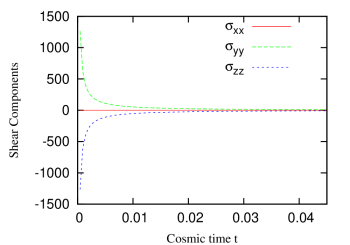
Figure 1: Shear Evolution for case $\Sigma_{1}=0$, $\Sigma_{2}=-\Sigma_{3}=0.05$.

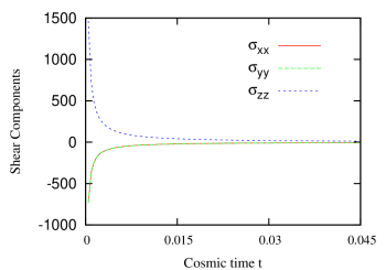
Figure 2: Shear Evolution for case $\Sigma_{1}=\Sigma_{2}=-0.05$, $\Sigma_{3}=0.1$.

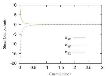
Figure 3: Shear Evolution for case $\Sigma_{1}=\Sigma_{2}=0.05$, $\Sigma_{3}=-0.1$.

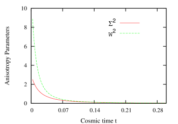
Figure 4: Anisotropy parameters $\Sigma^{2}$ and $\mathcal{W}^{2}$ for case $\Sigma_{1}=0$, $\Sigma_{2}=-\Sigma_{3}=0.05$

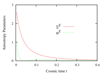
Figure 5: Anisotropy parameters $\Sigma^{2}$ and $\mathcal{W}^{2}$ for case $\Sigma_{1}=\Sigma_{2}=-0.05$, $\Sigma_{3}=0.1$

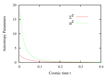
Figure 6: Anisotropy parameters $\Sigma^{2}$ and $\mathcal{W}^{2}$ for case $\Sigma_{1}=\Sigma_{2}=0.05$, $\Sigma_{3}=-0.1$

We conclude these components tend to zero, as we could expect from the equation for shear tensor we got before. However, the appropiate way to know if this model isotropize is to consider the evolution of two scalars $\Sigma^{2}$ and $\mathcal{W}^{2}$ [8] defined as:

$$\Sigma^{2}=\frac{\sigma_{\alpha\beta}\sigma^{\alpha\beta}}{6H^{2}},$$ (31)

$$\mathcal{W}^{2}=\frac{E_{\alpha\beta}E^{\alpha\beta}+H_{\alpha\beta}H^{\alpha\beta}}{6H^{4}}$$ (32)

These quantities are defined because the components of shear tensor are not dimensionless, they are normalized with the Hubble scalar $H$, and hence measuring the dynamical importance of the different variables with respect to the overall expansion of the universe.

When both parameters tend to zero we can say the model tends to isotropy. As was pointed out by [8], it was thought Bianchi $VII_{0}$ non-tilted dust model isotropize in the sense $\Sigma\rightarrow 0$ when $t\rightarrow\infty$. However, for $t\rightarrow\infty$ $\mathcal{W}\rightarrow\mathcal{W}_{0}$, where $\mathcal{W}_{0}$ is a constant whose value can be any positive number depending on the initial conditions [8]. On the contrary these two factors tend to zero for our three cases of Bianchi I model. We illustrate these behaviours in figures 4, 5 and 6.

We see these parameters tend to zero in the three cases we have considered, the model isotropize. In the first case, as the constant $\Sigma_{1}=0$, the shear component $\sigma_{xx}=0$. However, the electric component $E_{xx}$, which we have not plotted here but we showed in [14], is not identically zero, although it is very small, compared with the other Electric components. Both Electric and Shear tensors are diagonal. In the other cases, where there exists axial simmetry, it is reflected in the components of shear tensor.

3 Conclusions

We have shown the shear tensor in BI cosmology and we analized the solutions in the dust model. From our analysis it is clear is convenient to be careful when the covariant derivative is considered.

The anisotropy parameters show us that this model isotropize, for different cases. For late times $S(t)\alpha\ t^{2/3}$, $H\alpha\ t^{-1}$, $\sigma_{\alpha\beta}\sigma^{\alpha\beta}\alpha\ S(t)^{-6}\alpha\ t^{-4}$, so $\Sigma^{2}\alpha\ t^{-2}$, while $E_{\alpha\beta}E^{\alpha\beta}\alpha\ S(t)^{-12}$, so $\mathcal{W}^{2}\alpha\ t^{-8}$ and as we see in the plots, these parameters decay, given a well defined behavior of the kinematical quantities in BI cosmology.

References

• [1] G.F.R. Ellis and M.A.H. MacCallum. A class of homogeneous cosmological models, Commun. Math. Phys. 12 (1969) 108.
• [2] M.A.H. MacCallum and G.F.R. Ellis. A class of homogeneous cosmological models: II. Observations, Commun. Math. Phys. 19 (1970) 31.
• [3] G.F.R. Ellis and H. van Elst. Cosmological Models, in Carg se Lectures 1998, in Theoretical and Observational Cosmology, Ed. M. Lachi ze-Rey, Kluwer, Dordrecht 1999, 1. gr-qc/9812046.
• [4] H. van Elst Extensions and Applications of 1+3 Decomposition Methods in General Relativistic Cosmological Modelling, Ph.D. Thesis, Queen Mary and Westfield College, London, United Kingdom, 1996.
• [5] C.G. Tsagas, A. Challinor and R. Maartens. Relativistic Cosmology and Large Scale Structure, Phys. Rept. 465 (2008) 61, \arXivid0705.4397.
• [6] L. Campanelli, P. Cea and L. Tedesco. Phys. Rev. D 76 (2007) 063007, \arXivid0706.3802.
• [7] L. Campanelli, P. Cea and L. Tedesco. Ellipsoidal Universe Can Solve the Cosmic Microwave Background Quadrupole. Phys. Rev. Lett. 97 (2006) 131302; Phys. Rev. Lett. 97 (2006) 209903 (E).
• [8] U.S. Nilsson, C. Uggla, J. Wainwright and W.C. Lim. An Almost Isotropic Cosmic Microwave Temperature Does Not Imply an Almost Isotropic Universe, Astrophys. J. 521 (1999) L1-L3.
• [9] J. Wainwright and G.F.R. Ellis. Dynamical Systems in Cosmology, Cambridge University Press, Cambridge, 1997.
• [10] J. Ehlers. Akad. Wiss. Lit. Mainz. Abhandl. Math.-Nat. Kl. Nr. 11 (1961), in German. See english translation in Gen. Rel. Grav. 25 (1993) 1225.
• [11] K. Thorne. Primordial Element Formation, Primordial Magnetic Fields, and the Isotropy of the Universe, Astrophys. J. 148 (1967) 51.
• [12] S.W. Hawking and R.J. Tayler. Helium Production in an Anisotropic Big-Bang Cosmology Nature 209 (1966) 1278.
• [13] D.W. Olson. Helium Production and limits on the anisotropy of the Universe Astrophys. J. 219 (1978) 777.
• [14] Cáceres,D.L., Castaneda L. and Tejeiro J.M., Geodesic deviation equation in Bianchi Cosmologies, accepted for publication in Journal of Physics: Conference Series (JPCS), Spanish Relativity Meeting(ERE2009), \arXivid0912.4220.