Global Analysis of General $SU(2)\times SU(2)\times U(1)$ Models with Precision Data

Abstract

We present the results of a global analysis of a class of models with an extended electroweak gauge group of the form $SU(2)\times SU(2)\times U(1)$, often denoted as $G(221)$ models, which include as examples the left-right, the lepto-phobic, the hadro-phobic, the fermio-phobic, the un-unified, and the non-universal models. Using an effective Lagrangian approach, we compute the shifts to the coefficients in the electroweak Lagrangian due to the new heavy gauge bosons, and obtain the lower bounds on the masses of the $Z^{\prime}$ and $W^{\prime}$ bosons. The analysis of the electroweak parameter bounds reveals a consistent pattern of several key observables that are especially sensitive to the effects of new physics and thus dominate the overall shape of the respective parameter contours.

I Introduction

Despite the tremendous success of the Standard Model, there are still open questions that are unanswered and motivate further model-building. One of the most common model-building tools is to extend the gauge structure of the Standard Model. The simplest extension involves an additional $U(1)_{X}$ gauge symmetry (and thus an extra gauge boson $Z^{\prime}$). One of the next-simplest extensions involves an additional $SU(2)$, with the left-right model Mohapatra:1974gc Mohapatra:1974hk Mohapatra:1980yp being perhaps the most widely-studied case of such models. On the other hand, given the extended gauge group $SU(2)_{1}\times SU(2)_{2}\times U(1)_{X}$ in the electroweak sector, there are many other models besides the left-right model that can be constructed, and these models, despite having a common fundamental gauge group, may have very different low-energy phenomenology. In this paper we present a unified, systematic study of many such models, which are commonly called $G(221)$ models in the literature.

The most important feature of $G(221)$ models is the existence of new heavy gauge bosons, $W^{\prime}$ and $Z^{\prime}$. The existence of the gauge boson $Z^{\prime}$ has influences on the low-energy neutral-current processes, the $Z$-pole data at LEP-I and high energy LEP-II data Rizzo:2006nw Langacker:2008yv . The existence of the $W^{\prime}$ boson has implications to the search of new physics beyond the Standard Model (SM) via studying charged-current processes. In low energy experiments, the most sensitive probes of charged currents come from flavor physics, such as the $K\bar{K}$, $b\bar{b}$ mixing processes and semileptonic decays of the $b$ quark Langacker:1989xa Barenboim:1996nd . However, the low energy impact depends sensitively on the details of the flavor sectors, for which there is little experimental input Rizzo:1997ts . There is thus a large uncertainty on the constraints on $W^{\prime}$ and its interactions.

In this paper, we classify the $G(221)$ models by the patterns of symmetry breaking summarized in Table 2 (see section II). Our main goals are to obtain the bounds on the masses of the $W^{\prime}$ and $Z^{\prime}$ bosons for these various models, and, through the results of the global-fit analysis, to identify the key observables that are most sensitive to the new physics in these models. Our key results are that, at the 95% confidence level, the lower bounds on the masses of new heavy gauge bosons can be very light for breaking pattern I, which includes left-right, lepto-phobic, hadro-phobic and fermio-phobic models, for example, $M_{Z^{\prime}}\sim 1.6~{}\mbox{TeV}$ and $M_{W^{\prime}}\sim 0.3~{}\mbox{TeV}$ in the left-right model and hadro-phobic model; $M_{Z^{\prime}}\sim 1.7~{}\mbox{TeV}$ and $M_{W^{\prime}}\sim 0.7~{}\mbox{TeV}$ in the lepto-phobic and fermio-phobic models. In breaking pattern II, which includes un-unified and non-universial models, because of the degeneracy of the masses of the $W^{\prime}$ and $Z^{\prime}$, the lower bounds on their masses are quite heavy, for example, $M_{Z^{\prime}}=M_{W^{\prime}}\sim 2.5~{}\mbox{TeV}$ in the un-unified model.

We organize this paper as follows. In Section II, we lay out the various $G(221)$ models and discuss the results of the relevant literature. In Section III, we give the effective Lagrangians, both at the electroweak scale (obtained by integrating out $W^{\prime}$ and $Z^{\prime}$) and below the electroweak scale (by integrating out the $W$ and $Z$). In Section IV, we discuss the global-fit procedure and present our results obtained using the code Global Analysis for Particle Properties (GAPP) Erler:1999ug , a software that utilizes the CERN library MINUIT James:1975dr and was used for the Particle Data Group global analysis Amsler:2008zzb . We also discuss which observables are especially sensitive to the new physics contributions in these various models. We conclude in Section VI with a summary and outlook of our key findings. The Appendix contains the explicit effective Lagrangians for the $G(221)$ models.

II The $G(221)$ Models

We focus on the so-called $G(221)$ models having a $SU(2)_{1}\times SU(2)_{2}\times U(1)_{X}$ gauge structure that ultimately breaks to $U(1)_{\mbox{\tiny em}}$. Relative to the Standard Model, these models have three additional massive gauge bosons, and their phenomenology depends on the specific patterns of symmetry breaking as well as the charge assignments of the SM fermions. For our studies, we consider the following different $G(221)$ models: left-right (LR) Mohapatra:1974gc Mohapatra:1974hk Mohapatra:1980yp , lepto-phobic (LP), hadro-phobic (HP), fermio-phobic (FP) Chivukula:2006cg Barger:1980ix Barger:1980ti , un-unified (UU) Georgi:1989ic Georgi:1989xz , and non-universal (NU) Malkawi:1996fs Li:1981nk He:2002ha . The charge assignments of the SM fermions in these models are given in Table 1, and these models can be categorized by two patterns of symmetry breaking (summarized in Table 2):

• Breaking pattern I (the LR, LP, HP, and FP models):
  We identify $SU(2)_{1}$ as $SU(2)_{L}$ of the SM. The first stage of symmetry breaking then is $SU(2)_{2}\times U(1)_{X}\rightarrow U(1)_{Y}$, giving rise to three heavy gauge bosons $W^{\prime\pm}$ and $Z^{\prime}$ at the TeV-scale. The second stage is $SU(2)_{L}\times U(1)_{Y}\rightarrow U(1)_{\mbox{\tiny em}}$ at the electroweak scale.

• Breaking pattern II (the UU and NU models):
  We identify $U(1)_{X}$ as $U(1)_{Y}$ of the SM. The first stage of symmetry breaking is $SU(2)_{1}\times SU(2)_{2}\rightarrow SU(2)_{L}$. The second stage is $SU(2)_{L}\times U(1)_{Y}\rightarrow U(1)_{\mbox{\tiny em}}$ at the electroweak scale.

Table 1: The charge assignments of the SM fermions under the $G(221)$ gauge groups. Unless otherwise specified, the charge assignments apply to all three generations.

Model	$SU(2)_{1}$	$SU(2)_{2}$	$U(1)_{X}$
Left-right (LR)	$\begin{pmatrix}u_{\mbox{\tiny{$L$}}}\\ d_{\mbox{\tiny{$L$}}}\end{pmatrix},\begin{pmatrix}\nu_{\mbox{\tiny{$L$}}}\\ e_{\mbox{\tiny{$L$}}}\end{pmatrix}$	$\begin{pmatrix}u_{\mbox{\tiny{$R$}}}\\ d_{\mbox{\tiny{$R$}}}\end{pmatrix},\begin{pmatrix}\nu_{\mbox{\tiny{$R$}}}\\ e_{\mbox{\tiny{$R$}}}\end{pmatrix}$	$\begin{matrix}\tfrac{1}{6}\ \mbox{for quarks,}\\ -\tfrac{1}{2}\ \mbox{for leptons.}\end{matrix}$
Lepto-phobic (LP)	$\begin{pmatrix}u_{\mbox{\tiny{$L$}}}\\ d_{\mbox{\tiny{$L$}}}\end{pmatrix},\begin{pmatrix}\nu_{\mbox{\tiny{$L$}}}\\ e_{\mbox{\tiny{$L$}}}\end{pmatrix}$	$\begin{pmatrix}u_{\mbox{\tiny{$R$}}}\\ d_{\mbox{\tiny{$R$}}}\end{pmatrix}$	$\begin{matrix}\tfrac{1}{6}\ \mbox{for quarks,}\\ Y_{\mbox{\tiny SM}}\ \mbox{for leptons.}\end{matrix}$
Hadro-phobic (HP)	$\begin{pmatrix}u_{\mbox{\tiny{$L$}}}\\ d_{\mbox{\tiny{$L$}}}\end{pmatrix},\begin{pmatrix}\nu_{\mbox{\tiny{$L$}}}\\ e_{\mbox{\tiny{$L$}}}\end{pmatrix}$	$\begin{pmatrix}\nu_{\mbox{\tiny{$R$}}}\\ e_{\mbox{\tiny{$R$}}}\end{pmatrix}$	$\begin{matrix}Y_{\mbox{\tiny SM}}\ \mbox{for quarks,}\\ -\tfrac{1}{2}\ \mbox{for leptons.}\end{matrix}$
Fermio-phobic (FP)	$\begin{pmatrix}u_{\mbox{\tiny{$L$}}}\\ d_{\mbox{\tiny{$L$}}}\end{pmatrix},\begin{pmatrix}\nu_{\mbox{\tiny{$L$}}}\\ e_{\mbox{\tiny{$L$}}}\end{pmatrix}$		$\begin{matrix}Y_{\mbox{\tiny SM}}\ \mbox{for all fermions.}\end{matrix}$
Un-unified (UU)	$\begin{pmatrix}u_{\mbox{\tiny{$L$}}}\\ d_{\mbox{\tiny{$L$}}}\end{pmatrix}$	$\begin{pmatrix}\nu_{\mbox{\tiny{$L$}}}\\ e_{\mbox{\tiny{$L$}}}\end{pmatrix}$	$\begin{matrix}Y_{\mbox{\tiny SM}}\ \mbox{for all fermions.}\end{matrix}$
Non-universal (NU)	$\begin{pmatrix}u_{\mbox{\tiny{$L$}}}\\ d_{\mbox{\tiny{$L$}}}\end{pmatrix}_{1^{\mbox{\tiny st}},2^{\mbox{\tiny nd}}},\begin{pmatrix}\nu_{\mbox{\tiny{$L$}}}\\ e_{\mbox{\tiny{$L$}}}\end{pmatrix}_{1^{\mbox{\tiny st}},2^{\mbox{\tiny nd}}}$	$\begin{pmatrix}u_{\mbox{\tiny{$L$}}}\\ d_{\mbox{\tiny{$L$}}}\end{pmatrix}_{3^{\mbox{\tiny rd}}},\begin{pmatrix}\nu_{\mbox{\tiny{$L$}}}\\ e_{\mbox{\tiny{$L$}}}\end{pmatrix}_{3^{\mbox{\tiny rd}}}$	$\begin{matrix}Y_{\mbox{\tiny SM}}\ \mbox{for all fermions.}\end{matrix}$

Table 2: Summary of the two different breaking patterns and the two different stages of symmetry breaking in $G(221)$ models.

Pattern	Starting Point	First stage breaking	Second stage breaking
I	Identify $SU(2)_{1}$ as $SU(2)_{L}$	$SU(2)_{2}\times U(1)_{X}\rightarrow U(1)_{Y}$	$SU(2)_{L}\times U(1)_{Y}\rightarrow U(1)_{em}$
II	Identify $U(1)_{X}$ as $U(1)_{Y}$	$SU(2)_{1}\times SU(2)_{2}\rightarrow SU(2)_{L}$	$SU(2)_{L}\times U(1)_{Y}\rightarrow U(1)_{em}$

In addition to specifying the gauge group and the fermion charge assignments, a complete $G(221)$ model should also include the ingredients of the Higgs sectors and the Yukawa couplings. While the observed relationships between the masses of $W$ and $Z$ bosons leave little freedom in the Higgs representation used for electroweak symmetry breaking (EWSB), we have freedoms in the choices of the Higgs representation used to break the fundamental $G(221)$ gauge group to the SM gauge group. In breaking pattern I we assume the two simplest cases of symmetry breaking: via a doublet or a triplet Higgs. In the breaking pattern II we assume the simplest case of using a bi-doublet Higgs to achieve this symmetry breaking. The model-specific Higgs representations and vacuum expectation values (VEV’s) are given in Table 3. For heavy Higgs boson, Wang et al. Wang:2008nk used a non-linear effective theory approach to obtain an electroweak chiral Lagrangian for $W^{\prime}$. In our paper, by assuming a light Higgs, we analyze the low-energy constraints by using a linearlized effective Lagrangian approach.

First stage breaking
	Rep.	Multiplet and VEV
LR-D, LP-D HP-D, FP-D	$\Phi\sim(1,2,\tfrac{1}{2})$	$\Phi=\begin{pmatrix}\phi^{+}\\ \phi^{0}\end{pmatrix},\ \langle\Phi\rangle=\frac{\mbox{$1$}}{\mbox{$\sqrt{2}$}}\begin{pmatrix}0\\ \tilde{u}_{\mbox{\tiny D}}\end{pmatrix}$
LR-T, LP-T HP-T, FP-T	$\Phi\sim(1,3,1)$	$\Phi=\frac{1}{\sqrt{2}}\begin{pmatrix}\phi^{+}&\sqrt{2}\phi^{++}\\ \sqrt{2}\phi^{0}&-\phi^{+}\end{pmatrix},\ \langle\Phi\rangle=\frac{\mbox{$1$}}{\mbox{$\sqrt{2}$}}\begin{pmatrix}0&0\\ \tilde{u}_{\mbox{\tiny T}}&0\end{pmatrix}$
UU, NU	$\Phi\sim(2,\overline{2},0)$	$\Phi=\begin{pmatrix}\phi^{0}+\pi^{0}&\sqrt{2}\pi^{+}\\ \sqrt{2}\pi^{-}&\phi^{0}-\pi^{0}\end{pmatrix},\ \langle\Phi\rangle=\frac{\mbox{$1$}}{\mbox{$\sqrt{2}$}}\begin{pmatrix}\tilde{u}&0\\ 0&\tilde{u}\end{pmatrix}$

Second stage breaking
	Rep.	Multiplet and VEV
LR-D, LP-D HP-D, FP-D	$H\sim(2,\overline{2},0)$	$H=\begin{pmatrix}h_{1}^{0}&h_{1}^{+}\\ h_{2}^{-}&h_{2}^{0}\end{pmatrix}$, $\langle H\rangle=\frac{\mbox{$\tilde{v}$}}{\mbox{$\sqrt{2}$}}\begin{pmatrix}c_{\tilde{\beta}}&0\\ 0&s_{\tilde{\beta}}\end{pmatrix}$
LR-T, LP-T HP-T, FP-T	$H\sim(2,\overline{2},0)$	$H=\begin{pmatrix}h_{1}^{0}&h_{1}^{+}\\ h_{2}^{-}&h_{2}^{0}\end{pmatrix}$, $\langle H\rangle=\frac{\mbox{$\tilde{v}$}}{\mbox{$\sqrt{2}$}}\begin{pmatrix}c_{\tilde{\beta}}&0\\ 0&s_{\tilde{\beta}}\end{pmatrix}$
UU, NU	$H\sim(1,2,\tfrac{1}{2})$	$H=\begin{pmatrix}h^{+}\\ h^{0}\end{pmatrix}$, $\langle H\rangle=\frac{\mbox{$\tilde{v}$}}{\mbox{$\sqrt{2}$}}\begin{pmatrix}0\\ 1\end{pmatrix}$

Table 3: These tables display the model-specific Higgs representations and VEVs that achieve the symmetry breaking of $G(221)$ models.

The lepto-phobic, hadro-phobic, and un-unified models are, with the current set-up, incomplete because of gauge anomalies. It is entirely possible that the additional matter content used to address the anomalies can alter the low-energy phenomenologies and the results of our studies. Nevertheless, for completeness, we include these models with the current set-up in our studies, in which we focus on effects originated from the interactions of $W^{\prime}$ and $Z^{\prime}$ bosons to the SM fields. In the cases of the lepto-phobic and hadro-phobic models, one can view them as transitions between the left-right models (where both right-handed leptons and quarks are charged under $SU(2)_{2}$) and the fermio-phobic model (where neither are charged).

There have already been many theoretical and phenomenological studies of various $G(221)$ models, and we focus our brief literature review here mainly to those works that perform a global fitting in the same spirit as our work. In the symmetric left-right model (where the couplings of the $W^{\prime}$ are of the same strength as those of the $W$), Polak and Zralek obtained the constraints on parameters from the Z-pole data Polak:1991qw and low energy data Polak:1991pc , separately. While for the non-symmetric case, Chay, Lee and Nam Chay:1998hd considered phenomenological constraints on three parameters: the mass of the $Z^{\prime}$, the mixing angles $\tilde{\phi}$ (the analog of the Weinberg angle in the breaking of $SU(2)_{R}\times U(1)_{X}\rightarrow U(1)_{Y}$) and the $Z$-$Z^{\prime}$ mixing angle $\xi$, by combining the precision electroweak data from LEP I (through $\epsilon_{1},\epsilon_{2},\epsilon_{3}$) and the low-energy neutral-current experimental data. For the non-symmetric case, the combined bounds at the $95\%$ confidence level are $0.0028<\xi<0.0065$ and $M_{Z^{\prime}}\geq 400$ GeV for all $\tilde{\phi}$, while for the symmetric case, a more severe bound $M_{Z^{\prime}}\geq 1.6$ TeV is obtained.

In the fermio-phobic model, Donini et al. Donini:1997yu used the $Z$-pole and low-energy data, and the flavor physics data from flavor-changing neutral-current (FCNC) processes and $b\to s\gamma$, to put constraints on the parameter space ($W$-$W^{\prime}$ mixing angle $\alpha_{\pm}$, and $Z$-$Z^{\prime}$ mixing angle $\alpha_{0}$) by fixing several sets of representative values of $M_{W^{\prime}}$ and $x$ (strength of the coupling of the fermiophobic gauge group, relative to $SU(2)_{L}$ of the Standard Model). For the input parameters in the the ranges $100$ GeV $<M_{W^{\prime}}<1000$ GeV and $0.6<x<15$, and for a low Higgs mass of $100$ GeV, the best-fit values of $\left|\alpha_{0}\right|$ and $\left|\alpha_{\pm}\right|$ increases with increasing $x$, when holding $M_{W^{\prime}}$ fixed. On the other hand, when holding $x$ fixed, increasing $M_{W^{\prime}}$ leads to an increase in the best-fit values of $\left|\alpha_{0}\right|$ and a decrease in the best-fit values of $\left|\alpha_{\pm}\right|$. In the entire range of parameter space, the magnitude of the best-fit values of $\alpha_{0}$ and $\alpha_{\pm}$ are at the percent level.

In the non-unified model, Malkawi and Yuan Malkawi:1996fs performed a global fit of the parameter space $(x,\phi)$ using the Z-pole data, and found that the lower bound is $M_{Z^{\prime}}=M_{W^{\prime}}\geq 1.3\text{ TeV}$ if no flavor physics is included. Chivukula et. al Chivukula:1994qw used the data from precision electroweak measurements to put stringent bounds on the un-unified Standard Model Georgi:1989ic Georgi:1989xz . They found a lower bound on the masses of the heavy $W^{\prime}$ and $Z^{\prime}$ of approximately $2$ TeV at the $95\%$ confidence level.

III The Effective Lagrangian Approach

To analyze the low-energy constraints, we will take an effective Lagrangian approach, and follow the general procedures laid out by Burgess in Ref. Burgess:1993vc to extract the effects of new physics. Although the details of each of these models are different, we first perform a generic analysis that can be applied to any $G(221)$ model we consider in this work.

Per the convention in Burgess Burgess:1993vc , we denote the gauge couplings as $\tilde{g}_{1}$, $\tilde{g}_{2}$, and $\tilde{g}_{\mbox{\tiny{$X$}}}$ respectively for the gauge groups $SU(2)_{1}$, $SU(2)_{2}$, and $U(1)_{X}$. The tilde ($\tilde{\ }$) on the couplings and VEVs emphasizes the fact that these are model parameters, as opposed to quantities that can be directly measured in experiments, such as the physical mass of the $Z$ boson. As an extension to the convention in Burgess Burgess:1993vc , we also denote with tilde ($\tilde{\ }$) any combination constructed from the model parameters. We also abbreviate the trigonometric functions

$$c_{x}\equiv\cos(x),\ s_{x}\equiv\sin(x),\ \mbox{and}\ t_{x}\equiv\tan(x).$$ (1)

III.1 Mixing Angles and Gauge Couplings

We define the mixing angle $\tilde{\phi}$ at the first breaking stage as

$$t_{\tilde{\phi}}\left(=\tan\tilde{\phi}\right) \equiv\begin{cases}\tilde{g}_{\mbox{\tiny{$X$}}}/\tilde{g}_{2}&\mbox{(LR, LP, HP, FP models)}\\ \tilde{g}_{2}/\tilde{g}_{1}&\mbox{(UU, NU models)},\end{cases}$$ (2)

and define the couplings

$$\tilde{g}_{\mbox{\tiny{$L$}}} \equiv\begin{cases}\tilde{g}_{1},&\mbox{(LR, LP, HP, FP models)}\\ \left(\frac{\mbox{$1$}}{\mbox{$\tilde{g}_{1}^{2}$}}+\frac{\mbox{$1$}}{\mbox{$\tilde{g}_{2}^{2}$}}\right)^{-1/2}&\mbox{(UU, NU models)},\end{cases}$$

$$\tilde{g}_{\mbox{\tiny{$Y$}}} \equiv\begin{cases}\left(\frac{\mbox{$1$}}{\mbox{$\tilde{g}_{2}^{2}$}}+\frac{\mbox{$1$}}{\mbox{$\tilde{g}_{\mbox{\tiny{$X$}}}^{2}$}}\right)^{-1/2}&\mbox{(LR, LP, HP, FP models)}\\ \tilde{g}_{\mbox{\tiny{$X$}}},&\mbox{(UU, NU models)}.\end{cases}$$ (3)

The couplings $\tilde{g}_{\mbox{\tiny{$L$}}}$ and $\tilde{g}_{\mbox{\tiny{$Y$}}}$ are respectively the gauge couplings of the unbroken $SU(2)_{L}\times U(1)_{Y}$ gauge groups after the first stage of symmetry breaking. Similarly to the Standard Model, for both breaking patterns we define the weak mixing angle ($\tilde{\theta}$) as

$$t_{\tilde{\theta}}\left(=\tan\tilde{\theta}\right)\equiv\frac{\tilde{g}_{\mbox{\tiny{$Y$}}}}{\tilde{g}_{\mbox{\tiny{$L$}}}}.$$ (4)

For both breaking patterns, the electric charge ($\tilde{e}$) is given by

$$\frac{1}{\tilde{e}^{2}}=\frac{1}{\tilde{g}_{1}^{2}}+\frac{1}{\tilde{g}_{2}^{2}}+\frac{1}{\tilde{g}_{\mbox{\tiny{$X$}}}^{2}},$$ (5)

and we also define $\tilde{\alpha}_{e}\equiv\tilde{e}^{2}/4\pi$.

With the angles $\tilde{\theta}$ and $\tilde{\phi}$, the gauge couplings can be expressed as

$$\tilde{g}_{1} =\begin{cases}\tilde{e}/(s_{\tilde{\theta}}),&\mbox{(LR, LP, HP, FP models)}\\ \tilde{e}/(s_{\tilde{\theta}}s_{\tilde{\phi}}),&\mbox{(UU, NU models)}\end{cases}$$ (6)

$$\tilde{g}_{2} =\begin{cases}\tilde{e}/(c_{\tilde{\theta}}s_{\tilde{\phi}}),&\mbox{(LR, LP, HP, FP models)}\\ \tilde{e}/(s_{\tilde{\theta}}c_{\tilde{\phi}}),&\mbox{(UU, NU models)}\end{cases}$$ (7)

$$\tilde{g}_{\mbox{\tiny{$X$}}} =\begin{cases}\tilde{e}/(c_{\tilde{\theta}}c_{\tilde{\phi}}),&\mbox{(LR, LP, HP, FP models)}\\ \tilde{e}/(c_{\tilde{\theta}}).&\mbox{(UU, NU models)}\end{cases}$$ (8)

III.2 The Effective Lagrangian

III.2.1 Gauge Interactions of Fermions

In this sub-section we parameterize the gauge interactions of the fermions that is applicable to all the $G(221)$ models under considerations here. We will obtain both the SM-like effective theory applicable at the electroweak scale as well as the four-fermion effective theory below the electroweak scale. We do this by first building up the fundamental Lagrangian in stages, and then successively integrating out the massive gauge bosons. The $Z$-pole data measured at the electroweak scale, and measurements of the four-fermion neutral-current interactions are some of the most precise measurements to-date, and provide stringent bounds on new physics models.

As discussed earlier, we consider the symmetry breaking to take two stages:

$$SU(2)_{1}\times SU(2)_{2}\times U(1)_{X}\rightarrow SU(2)_{L}\times U(1)_{Y}\rightarrow U(1)_{\mbox{\tiny em}}.$$ (9)

We denote the gauge bosons of the $G(221)$ models as:

$$SU(2)_{1} :W_{1,\mu}^{\pm},W_{1,\mu}^{3},$$

$$SU(2)_{2} :W_{2,\mu}^{\pm},W_{2,\mu}^{3},$$

$$U(1)_{X} :X_{\mu}.$$ (10)

After the first-stage breaking, the neutral gauge eigenstates mix as follows

$$\hat{B}_{\mu} \equiv\begin{cases}s_{\tilde{\phi}}W^{3}_{2,\mu}+c_{\tilde{\phi}}X_{\mu}&\mbox{(LR, LP, HP, FP models)}\\ X_{\mu}&\mbox{(UU, NU models)}\end{cases}$$

$$\hat{W}^{3}_{\mu} \equiv\begin{cases}W_{1,\mu}^{3}&\mbox{(LR, LP, HP, FP models)}\\ s_{\tilde{\phi}}W^{3}_{1,\mu}+c_{\tilde{\phi}}W^{3}_{2,\mu}&\mbox{(UU, NU models)}\end{cases}$$

$$\hat{Z}^{\prime}_{\mu} \equiv\begin{cases}c_{\tilde{\phi}}W^{3}_{2,\mu}-s_{\tilde{\phi}}X_{\mu}&\mbox{(LR, LP, HP, FP models)}\\ c_{\tilde{\phi}}W^{3}_{1,\mu}-s_{\tilde{\phi}}W^{3}_{2,\mu},&\mbox{(UU, NU models)}\end{cases}$$ (11)

and for the charged gauge bosons, we have

$$\hat{W}_{\mu}^{\pm} \equiv\begin{cases}W^{\pm}_{1,\mu}&\mbox{(LR, LP, HP, FP models)}\\ s_{\tilde{\phi}}W^{\pm}_{1,\mu}+c_{\tilde{\phi}}W^{\pm}_{2,\mu},&\mbox{(UU, NU models)}\end{cases}$$

$$\hat{W}^{\prime\pm}_{\mu} \equiv\begin{cases}W^{\pm}_{2,\mu},&\mbox{(LR, LP, HP, FP models)}\\ c_{\tilde{\phi}}W^{\pm}_{1,\mu}-s_{\tilde{\phi}}W^{\pm}_{2,\mu}.&\mbox{(UU, NU models)}\end{cases}$$ (12)

After the first stage of symmetry breaking, there is still an unbroken $SU(2)_{L}\times U(1)_{Y}$, which may be identified as the Standard Model gauge group. The gauge bosons $\hat{W}^{\pm,3}$ and $\hat{B}$ are massless, and only $\hat{Z}^{\prime}$ and $\hat{W}^{\prime\pm}$ are massive, with TeV-scale masses. The Lagrangian representing the heavy gauge boson masses has the form

$$\mathcal{L}^{\mbox{\tiny stage-1}} =\frac{1}{2}\widetilde{M}^{2}_{Z^{\prime}}\hat{Z}^{\prime}_{\mu}\hat{Z}^{\prime\mu}+\widetilde{M}^{2}_{W^{\prime}}\hat{W}^{\prime+}_{\mu}\hat{W}^{\prime-\mu},$$ (13)

where $\widetilde{M}^{2}_{Z^{\prime}}$ and $\widetilde{M}^{2}_{W^{\prime}}$ are given in Table 6.

Before discussing the second stage of symmetry breaking, it is convenient to define, similarly to the Standard Model, $A_{\mu}$ (which will turn out to be the photon) and $\hat{Z}_{\mu}$ (approximately the physical $Z$-boson) in terms of the massless gauge bosons $\hat{W}^{3}_{\mu}$ and $\hat{B}_{\mu}$

$$A_{\mu} \equiv\left(\frac{\tilde{e}}{\tilde{g}_{1}}W^{3}_{1,\mu}+\frac{\tilde{e}}{\tilde{g}_{2}}W^{3}_{2,\mu}+\frac{\tilde{e}}{\tilde{g}_{\mbox{\tiny{$X$}}}}\hat{X}_{\mu}\right),$$

$$=s_{\tilde{\theta}}\hat{W}^{3}_{\mu}+c_{\tilde{\theta}}\hat{B}_{\mu},$$

$$\hat{Z}_{\mu} \equiv c_{\tilde{\theta}}\hat{W}^{3}_{\mu}-s_{\tilde{\theta}}\hat{B}_{\mu},$$ (14)

At the electroweak scale, the second stage of symmetry breaking takes place, breaking $SU(2)\times U(1)\rightarrow U(1)_{\mbox{\tiny em}}$. The Higgs vacuum expectation value (VEV) at the second stage not only gives masses to $\hat{Z}$ and $\hat{W}^{\pm}$, but also induces further mixing among the gauge bosons $\hat{W}^{\pm}$, $\hat{Z}$, $\hat{W}^{\prime}$ and $\hat{Z}^{\prime}$. The masses of the gauge bosons depend not only on the breaking pattern, but also on the group representations of the Higgs bosons whose VEV’s trigger the symmetry breaking. For simplicity, for breaking pattern I, we consider only models with either a doublet or triplet under $SU(2)_{2}$, and do not consider models with both doublets and triplets. Introducing additional Higgses and VEVs would modify the masses of the $W^{\prime}$ and $Z^{\prime}$ Polak:1991vf . For breaking pattern II, since the first stage of symmetry breaking breaks $SU(2)_{1}\times SU(2)_{2}$ to the diagonal subgroup, the masses of $W^{\prime}$ and $Z^{\prime}$ are degenerate at this stage, and we only consider the case of an $SU(2)_{1}\times SU(2)_{2}$ bi-doublet. For the convenience of typesetting, we also denote, for example, a left-right model with first-stage symmetry breaking triggered by an $SU(2)$-doublet(-triplet) as LR-D (LR-T).

Although different breaking patterns and different group representations of the Higgs bosons will lead to different Lagrangians, we can write down the Lagrangian involving the gauge boson masses and fermionic gauge interactions in a general form

$$\mathcal{L}_{\mbox{\tiny fund}} =\frac{1}{2}\widetilde{M}^{2}_{Z}\hat{Z}_{\mu}\hat{Z}^{\mu}+\frac{1}{2}(\widetilde{M}^{2}_{Z^{\prime}}+\Delta\widetilde{M}^{2}_{Z^{\prime}})\hat{Z}^{\prime}_{\mu}\hat{Z}^{\prime\mu}+\delta\widetilde{M}^{2}_{Z}\hat{Z}^{\prime}_{\mu}\hat{Z}^{\mu}$$

$$\ +\widetilde{M}^{2}_{W}\hat{W}^{+}_{\mu}\hat{W}^{-\mu}+(\widetilde{M}^{2}_{W^{\prime}}+\Delta\widetilde{M}^{2}_{W^{\prime}})\hat{W}^{\prime+}_{\mu}\hat{W}^{\prime-\mu}+\delta\widetilde{M}^{2}_{W}(\hat{W}^{\prime+}_{\mu}\hat{W}^{-\mu}+\hat{W}^{\prime-}_{\mu}\hat{W}^{+\mu})$$

$$\ +\hat{W}_{\mu}^{\prime+}K^{+\mu}+\hat{W}_{\mu}^{\prime-}K^{-\mu}+\hat{Z}_{\mu}^{\prime}K^{0\mu}$$

$$\ +\hat{W}_{\mu}^{+}J^{+\mu}+\hat{W}_{\mu}^{-}J^{-\mu}+\hat{Z}_{\mu}J^{0\mu}+A_{\mu}J^{\mu},$$ (15)

where we have denoted the currents that couple to the primed gauge bosons ($\hat{W}^{\prime}$ and $\hat{Z}^{\prime}$) as $K^{0}_{\mu}$ and $K_{\mu}^{\pm}$, and the currents that couple to the SM gauge bosons as $J_{\mu}$, $J^{0}_{\mu}$ and $J^{\pm}_{\mu}$. The SM-like currents have the familiar forms

$$J^{\mu} =\tilde{e}\sum\limits_{f}Q^{f}\overline{f}\gamma^{\mu}f,$$ (16)

$$J^{0}_{\mu} =\sqrt{\tilde{g}_{\mbox{\tiny{$L$}}}^{2}+\tilde{g}_{\mbox{\tiny{$Y$}}}^{2}}\ \sum\limits_{f}\left(T_{3L}^{f}\overline{f}_{\mbox{\tiny L}}\gamma_{\mu}P_{\mbox{\tiny L}}f_{\mbox{\tiny L}}-s_{\tilde{\theta}}^{2}Q^{f}\ \overline{f}\gamma_{\mu}f\right),$$ (17)

$$J^{+}_{\mu} =\frac{\tilde{g}_{\mbox{\tiny{$L$}}}}{\sqrt{2}}\left(\overline{d}_{\mbox{\tiny L}}\gamma_{\mu}P_{\mbox{\tiny L}}u_{\mbox{\tiny L}}+\overline{e}_{\mbox{\tiny L}}\gamma_{\mu}P_{\mbox{\tiny L}}\nu_{\mbox{\tiny L}}\right),$$ (18)

with an implicit sum over the three generations of fermions. The neutral currents ($K^{0}_{\mu}$) and charged currents ($K_{\mu}^{\pm}$), for the various models are summarized in Tables 4 and 5.

	$\overline{u}\gamma^{\mu}u$	$\overline{d}\gamma^{\mu}d$	$\overline{\nu}\gamma^{\mu}\nu$	$\overline{e}\gamma^{\mu}e$
LR	$\begin{matrix}(\tfrac{1}{2}c_{\tilde{\phi}}\tilde{g}_{2}-\tfrac{1}{6}s_{\tilde{\phi}}\tilde{g}_{\mbox{\tiny{$X$}}})P_{\mbox{\tiny R}}\\ -\frac{1}{6}s_{\tilde{\phi}}\tilde{g}_{\mbox{\tiny{$X$}}}P_{\mbox{\tiny L}}\end{matrix}$	$\begin{matrix}(-\tfrac{1}{2}c_{\tilde{\phi}}\tilde{g}_{2}-\tfrac{1}{6}s_{\tilde{\phi}}\tilde{g}_{\mbox{\tiny{$X$}}})P_{\mbox{\tiny R}}\\ -\frac{1}{6}s_{\tilde{\phi}}\tilde{g}_{\mbox{\tiny{$X$}}}P_{\mbox{\tiny L}}\end{matrix}$	$\begin{matrix}(\tfrac{1}{2}c_{\tilde{\phi}}\tilde{g}_{2}+\tfrac{1}{2}s_{\tilde{\phi}}\tilde{g}_{\mbox{\tiny{$X$}}})P_{\mbox{\tiny R}}\\ +\frac{1}{2}s_{\tilde{\phi}}\tilde{g}_{\mbox{\tiny{$X$}}}P_{\mbox{\tiny L}}\end{matrix}$	$\begin{matrix}(-\tfrac{1}{2}c_{\tilde{\phi}}\tilde{g}_{2}+\tfrac{1}{2}s_{\tilde{\phi}}\tilde{g}_{\mbox{\tiny{$X$}}})P_{\mbox{\tiny R}}\\ +\frac{1}{2}s_{\tilde{\phi}}\tilde{g}_{\mbox{\tiny{$X$}}}P_{\mbox{\tiny L}}\end{matrix}$
LP	$\begin{matrix}(\tfrac{1}{2}c_{\tilde{\phi}}\tilde{g}_{2}-\tfrac{1}{6}s_{\tilde{\phi}}\tilde{g}_{\mbox{\tiny{$X$}}})P_{\mbox{\tiny R}}\\ -\frac{1}{6}s_{\tilde{\phi}}\tilde{g}_{\mbox{\tiny{$X$}}}P_{\mbox{\tiny L}}\end{matrix}$	$\begin{matrix}(-\tfrac{1}{2}c_{\tilde{\phi}}\tilde{g}_{2}-\tfrac{1}{6}s_{\tilde{\phi}}\tilde{g}_{\mbox{\tiny{$X$}}})P_{\mbox{\tiny R}}\\ -\frac{1}{6}s_{\tilde{\phi}}\tilde{g}_{\mbox{\tiny{$X$}}}P_{\mbox{\tiny L}}\end{matrix}$	$\frac{1}{2}s_{\tilde{\phi}}\tilde{g}_{\mbox{\tiny{$X$}}}P_{\mbox{\tiny L}}$	$s_{\tilde{\phi}}\tilde{g}_{\mbox{\tiny{$X$}}}(\frac{1}{2}P_{\mbox{\tiny L}}+P_{\mbox{\tiny R}})$
HP	$-s_{\tilde{\phi}}\tilde{g}_{\mbox{\tiny{$X$}}}(\tfrac{1}{6}P_{\mbox{\tiny L}}+\frac{2}{3}P_{\mbox{\tiny R}})$	$-s_{\tilde{\phi}}\tilde{g}_{\mbox{\tiny{$X$}}}(\tfrac{1}{6}P_{\mbox{\tiny L}}-\frac{1}{3}P_{\mbox{\tiny R}})$	$\begin{matrix}(\tfrac{1}{2}c_{\tilde{\phi}}\tilde{g}_{2}+\tfrac{1}{2}s_{\tilde{\phi}}\tilde{g}_{\mbox{\tiny{$X$}}})P_{\mbox{\tiny R}}\\ +\frac{1}{2}s_{\tilde{\phi}}\tilde{g}_{\mbox{\tiny{$X$}}}P_{\mbox{\tiny L}}\end{matrix}$	$\begin{matrix}(-\tfrac{1}{2}c_{\tilde{\phi}}\tilde{g}_{2}+\tfrac{1}{2}s_{\tilde{\phi}}\tilde{g}_{\mbox{\tiny{$X$}}})P_{\mbox{\tiny R}}\\ +\frac{1}{2}s_{\tilde{\phi}}\tilde{g}_{\mbox{\tiny{$X$}}}P_{\mbox{\tiny L}}\end{matrix}$
FP	$-s_{\tilde{\phi}}\tilde{g}_{\mbox{\tiny{$X$}}}(\tfrac{1}{6}P_{\mbox{\tiny L}}+\frac{2}{3}P_{\mbox{\tiny R}})$	$-s_{\tilde{\phi}}\tilde{g}_{\mbox{\tiny{$X$}}}(\tfrac{1}{6}P_{\mbox{\tiny L}}-\frac{1}{3}P_{\mbox{\tiny R}})$	$\frac{1}{2}s_{\tilde{\phi}}\tilde{g}_{\mbox{\tiny{$X$}}}P_{\mbox{\tiny L}}$	$s_{\tilde{\phi}}\tilde{g}_{\mbox{\tiny{$X$}}}(\frac{1}{2}P_{\mbox{\tiny L}}+P_{\mbox{\tiny R}})$
UU	$\tfrac{1}{2}c_{\tilde{\phi}}\tilde{g}_{1}P_{\mbox{\tiny L}}$	$-\tfrac{1}{2}c_{\tilde{\phi}}\tilde{g}_{1}P_{\mbox{\tiny L}}$	$-\tfrac{1}{2}s_{\tilde{\phi}}\tilde{g}_{2}P_{\mbox{\tiny L}}$	$\tfrac{1}{2}s_{\tilde{\phi}}\tilde{g}_{2}P_{\mbox{\tiny L}}$
NU	$\frac{1}{2}\begin{pmatrix}c_{\tilde{\phi}}\tilde{g}_{1}\\ -s_{\tilde{\phi}}\tilde{g}_{2}\end{pmatrix}P_{\mbox{\tiny L}}$	$-\frac{1}{2}\begin{pmatrix}c_{\tilde{\phi}}\tilde{g}_{1}\\ -s_{\tilde{\phi}}\tilde{g}_{2}\end{pmatrix}P_{\mbox{\tiny L}}$	$\frac{1}{2}\begin{pmatrix}c_{\tilde{\phi}}\tilde{g}_{1}\\ -s_{\tilde{\phi}}\tilde{g}_{2}\end{pmatrix}P_{\mbox{\tiny L}}$	$-\frac{1}{2}\begin{pmatrix}c_{\tilde{\phi}}\tilde{g}_{1}\\ -s_{\tilde{\phi}}\tilde{g}_{2}\end{pmatrix}P_{\mbox{\tiny L}}$

Table 4: This table displays the couplings $\tilde{g}(\overline{f},f,\hat{Z}^{\prime})$ of the current $K^{0\mu}=\overline{f}\gamma^{\mu}\tilde{g}(\overline{f},f,\hat{Z}^{\prime})f$. For the top four models (LR, LP, HP, and FP), $\tan\phi\equiv\tilde{g}_{\mbox{\tiny{$X$}}}/\tilde{g}_{2}$. For the lower two models (UU and NU), $\tan\phi\equiv\tilde{g}_{2}/\tilde{g}_{1}$. For the NU model (last row), the top values denote the couplings to the first two generations of fermions, and the bottom values denote the couplings to the third generation.

	$\overline{d}\gamma^{\mu}u$	$\overline{e}\gamma^{\mu}\nu$
LR	$\frac{1}{\sqrt{2}}\tilde{g}_{2}P_{\mbox{\tiny R}}$	$\frac{1}{\sqrt{2}}\tilde{g}_{2}P_{\mbox{\tiny R}}$
LP	$\frac{1}{\sqrt{2}}\tilde{g}_{2}P_{\mbox{\tiny R}}$	0
HP	0	$\frac{1}{\sqrt{2}}\tilde{g}_{2}P_{\mbox{\tiny R}}$
FP	0	0
UU	$\tfrac{1}{\sqrt{2}}c_{\tilde{\phi}}\tilde{g}_{1}P_{\mbox{\tiny L}}$	$-\tfrac{1}{\sqrt{2}}s_{\tilde{\phi}}\tilde{g}_{2}P_{\mbox{\tiny L}}$
NU	$\frac{1}{\sqrt{2}}\begin{pmatrix}c_{\tilde{\phi}}\tilde{g}_{1}\\ -s_{\tilde{\phi}}\tilde{g}_{2}\end{pmatrix}P_{\mbox{\tiny L}}$	$\frac{1}{\sqrt{2}}\begin{pmatrix}c_{\tilde{\phi}}\tilde{g}_{1}\\ -s_{\tilde{\phi}}\tilde{g}_{2}\end{pmatrix}P_{\mbox{\tiny L}}$

Table 5: This table displays the couplings $\tilde{g}(\overline{\psi},\xi,\hat{W}^{\prime+})$ of the current $K^{+\mu}=\overline{\psi}\gamma^{\mu}\tilde{g}(\overline{\psi},\xi,\hat{W}^{\prime+})\xi$. For the top four models (LR, LP, HP, and FP), $\tan\phi\equiv\tilde{g}_{\mbox{\tiny{$X$}}}/\tilde{g}_{2}$. For the lower two models (UU and NU), $\tan\phi\equiv\tilde{g}_{2}/\tilde{g}_{1}$. For the NU model (last row), the top values denote the couplings to the first two generations of fermions, and the bottom values denote the couplings to the third generation.

We note the following features:

• The residual $SU(2)_{L}\times U(1)_{Y}$ is broken to the $U(1)_{\mbox{\tiny em}}$, and there are now mass terms for the $\hat{Z}$ and $\hat{W}$ bosons, denoted as $\widetilde{M}_{Z,W}^{2}$. These masses have the familiar form

  $$\widetilde{M}_{Z}^{2} =\frac{1}{4}({\tilde{g}_{\mbox{\tiny{$L$}}}}^{2}+{\tilde{g}_{\mbox{\tiny{$Y$}}}}^{2})\widetilde{v}^{2},$$ (19)

  $$\widetilde{M}_{W}^{2} =\frac{1}{4}{\tilde{g}_{\mbox{\tiny{$L$}}}}^{2}\widetilde{v}^{2},$$ (20)

  where the couplings $\tilde{g}_{\mbox{\tiny{$L$}}}$ and $\tilde{g}_{\mbox{\tiny{$Y$}}}$ are defined as in Eq. (3) for the two different breaking patterns.

• There are mass-mixing contributions $\delta\widetilde{M}^{2}_{Z,W}$ that induce $\hat{Z}-\hat{Z}^{\prime}$ and $\hat{W}-\hat{W}^{\prime}$ mixing. They are dependent on the breaking pattern and are given in Table 6.

• There are additional contributions to the masses of the $\hat{Z}^{\prime}$ and $\hat{W}^{\prime}$ after the second stage of symmetry breaking, which we denote as $\Delta\widetilde{M}^{2}_{Z^{\prime},W^{\prime}}$. They are also dependent on the breaking pattern and are given in Table 6.

	$\widetilde{M}^{2}_{Z^{\prime}}$	$\widetilde{M}^{2}_{W^{\prime}}$	$\Delta\widetilde{M}^{2}_{Z^{\prime}}$	$\Delta\widetilde{M}^{2}_{W^{\prime}}$	$\delta\widetilde{M}^{2}_{Z}$	$\delta\widetilde{M}^{2}_{W}$
LR-D, LP-D HP-D, FP-D	$\frac{\mbox{$1$}}{\mbox{$4$}}(\tilde{g}_{2}^{2}+\tilde{g}_{\mbox{\tiny{$X$}}}^{2})\tilde{u}_{\mbox{\tiny D}}^{2}$	$\frac{\mbox{$1$}}{\mbox{$4$}}\tilde{g}_{2}^{2}\tilde{u}_{\mbox{\tiny D}}^{2}$	$\frac{\mbox{$c^{2}_{\tilde{\phi}}$}}{\mbox{$4$}}\tilde{g}_{2}^{2}\tilde{v}^{2}$	$\frac{\mbox{$1$}}{\mbox{$4$}}\tilde{g}_{2}^{2}\tilde{v}^{2}$	$-\frac{\mbox{$c_{\tilde{\phi}}^{2}$}}{\mbox{$4\tilde{e}$}}\tilde{g}_{1}\tilde{g}_{2}\tilde{g}_{\mbox{\tiny{$X$}}}\tilde{v}^{2}$	$-\frac{\mbox{$1$}}{\mbox{$4$}}\tilde{g}_{1}\tilde{g}_{2}\tilde{v}^{2}s_{2\tilde{\beta}}$
LR-T, LP-T HP-T, FP-T	$(\tilde{g}_{2}^{2}+\tilde{g}_{\mbox{\tiny{$X$}}}^{2})\tilde{u}_{\mbox{\tiny T}}^{2}$	$\frac{\mbox{$1$}}{\mbox{$2$}}\tilde{g}_{2}^{2}\tilde{u}_{\mbox{\tiny T}}^{2}$	$\frac{\mbox{$c^{2}_{\tilde{\phi}}$}}{\mbox{$4$}}\tilde{g}_{2}^{2}\tilde{v}^{2}$	$\frac{\mbox{$1$}}{\mbox{$4$}}\tilde{g}_{2}^{2}\tilde{v}^{2}$	$-\frac{\mbox{$c_{\tilde{\phi}}^{2}$}}{\mbox{$4\tilde{e}$}}\tilde{g}_{1}\tilde{g}_{2}\tilde{g}_{\mbox{\tiny{$X$}}}\tilde{v}^{2}$	$-\frac{\mbox{$1$}}{\mbox{$4$}}\tilde{g}_{1}\tilde{g}_{2}\tilde{v}^{2}s_{2\tilde{\beta}}$
UU, NU	$\frac{\mbox{$1$}}{\mbox{$4$}}(\tilde{g}_{1}^{2}+\tilde{g}_{2}^{2})\tilde{u}^{2}$	$\frac{\mbox{$1$}}{\mbox{$4$}}(\tilde{g}_{1}^{2}+\tilde{g}_{2}^{2})\tilde{u}^{2}$	$\frac{\mbox{$s^{2}_{\tilde{\phi}}$}}{\mbox{$4$}}\tilde{g}_{2}^{2}\tilde{v}^{2}$	$\frac{\mbox{$s^{2}_{\tilde{\phi}}$}}{\mbox{$4$}}\tilde{g}_{2}^{2}\tilde{v}^{2}$	$-\frac{\mbox{$s_{\tilde{\phi}}^{2}$}}{\mbox{$4\tilde{e}$}}\tilde{g}_{1}\tilde{g}_{2}\tilde{g}_{\mbox{\tiny{$X$}}}\tilde{v}^{2}$	$-\frac{\mbox{$1$}}{\mbox{$4$}}\tilde{g}_{1}\tilde{g}_{2}\tilde{v}^{2}s^{2}_{\tilde{\phi}}$

Table 6: This table displays the model-dependent parameters $\widetilde{M}^{2}_{Z^{\prime},W^{\prime}}$ in Eq. (13), and $\Delta\widetilde{M}^{2}_{Z^{\prime},W^{\prime}}$ and $\delta\widetilde{M}^{2}_{Z,W}$ in Eq. (15).

Therefore, the gauge boson mass terms can be written as

$$\mathcal{L}_{\mbox{\tiny mass}} = \left(\begin{array}[]{cc}\hat{W}^{+}_{\mu}&\hat{W}^{\prime+}_{\mu}\end{array}\right)\left(\begin{array}[]{cc}\widetilde{M}^{2}_{W}&\delta\widetilde{M}^{2}_{W}\\ \delta\widetilde{M}^{2}_{W}&\widetilde{M}^{2}_{W^{\prime}}+\Delta\widetilde{M}^{2}_{W^{\prime}}\end{array}\right)\left(\begin{array}[]{c}\hat{W}^{-\mu}\\ \hat{W}^{\prime-\mu}\end{array}\right)$$ (26)

$$+ \frac{1}{2}\left(\begin{array}[]{ccc}A&\hat{Z}_{\mu}&\hat{Z}^{\prime}_{\mu}\end{array}\right)\left(\begin{array}[]{ccc}0&0&0\\ 0&\widetilde{M}^{2}_{Z}&\delta\widetilde{M}^{2}_{Z}\\ 0&\delta\widetilde{M}^{2}_{Z}&\widetilde{M}^{2}_{Z^{\prime}}+\Delta\widetilde{M}^{2}_{Z^{\prime}}\end{array}\right)\left(\begin{array}[]{c}A\\ \hat{Z}^{\mu}\\ \hat{Z}^{\prime\mu}\end{array}\right)\,.$$ (34)

In Table 3, we expect that the scale $\tilde{u}^{2}$ of the first-stage breaking is much larger than the electroweak scale $\tilde{v}^{2}$. We work to leading order in $\tilde{v}^{2}/\tilde{u}^{2}$, and so if we take the approximation

$$\widetilde{M}^{2}_{Z^{\prime},W^{\prime}}\gg\widetilde{M}^{2}_{Z,W},\delta\widetilde{M}^{2}_{Z,W},\Delta\widetilde{M}^{2}_{Z,W},$$ (35)

we can expand in large $\widetilde{M}^{2}_{Z^{\prime},W^{\prime}}$. To order $\mathcal{O}(\widetilde{M}^{-2}_{W^{\prime},Z^{\prime}})$, the mass eigenstates, denoted without the hats ($\hat{\ }$), are given by (similarly for the charged gauge bosons):

$$Z_{\mu} \equiv\hat{Z}_{\mu}-\frac{\delta\widetilde{M}^{2}_{Z}}{\widetilde{M}^{2}_{Z^{\prime}}-\widetilde{M}^{2}_{Z}}\hat{Z}^{\prime}_{\mu},$$ (36)

$$Z_{\mu}^{\prime} \equiv\frac{\delta\widetilde{M}^{2}_{Z}}{\widetilde{M}^{2}_{Z^{\prime}}-\widetilde{M}^{2}_{Z}}\hat{Z}_{\mu}+\hat{Z}^{\prime}_{\mu}.$$ (37)

Now we can rewrite the fundamental Lagrangian in terms of the mass eigenstates for both neutral and charged gauge bosons

$$\mathcal{L}^{\mbox{\tiny mass}}_{\mbox{\tiny fund}} =\frac{1}{2}\left(\widetilde{M}_{Z}^{2}-\frac{\delta\widetilde{M}^{4}_{Z}}{\widetilde{M}^{2}_{Z^{\prime}}}\right)Z_{\mu}Z^{\mu}+\left(\widetilde{M}^{2}_{W}-\frac{\delta\widetilde{M}^{4}_{W}}{\widetilde{M}^{2}_{W^{\prime}}}\right)W^{+\mu}W^{-}_{\mu}$$

$$\ +\frac{1}{2}\left(\widetilde{M}_{Z^{\prime}}^{2}+\Delta\widetilde{M}^{2}_{Z^{\prime}}+\frac{\delta\widetilde{M}^{4}_{Z}}{\widetilde{M}^{2}_{Z^{\prime}}}\right)Z^{\prime}_{\mu}Z^{\prime\mu}+\left(\widetilde{M}^{2}_{W^{\prime}}+\Delta\widetilde{M}^{2}_{W^{\prime}}+\frac{\delta\widetilde{M}^{4}_{W}}{\widetilde{M}^{2}_{W^{\prime}}}\right)W^{\prime+\mu}W^{\prime-}_{\mu}$$

$$\ +Z_{\mu}\left(J^{0\mu}-\frac{\delta\widetilde{M}^{2}_{Z}}{\widetilde{M}^{2}_{Z^{\prime}}}K^{0\mu}\right)+Z^{\prime}_{\mu}\left(K^{0\mu}+\frac{\delta\widetilde{M}^{2}_{Z}}{\widetilde{M}^{2}_{Z^{\prime}}}J^{0\mu}\right)+A_{\mu}J^{\mu}$$

$$\ +\left[W_{\mu}^{+}\left(J^{+\mu}-\frac{\delta\widetilde{M}^{2}_{W}}{\widetilde{M}^{2}_{W^{\prime}}}K^{+\mu}\right)+W_{\mu}^{\prime+}\left(K^{+\mu}+\frac{\delta\widetilde{M}^{2}_{W}}{\widetilde{M}^{2}_{W^{\prime}}}J^{+\mu}\right)+(+\leftrightarrow-)\right].$$ (38)

We can now obtain the effective Lagrangian by successively integrating out the massive gauge bosons. In the basis of the mass eigenstates, integrating out $Z^{\prime}$ and $W^{\prime}$ (whose masses are expected to be at or above the TeV scale) results in an effective Lagrangian valid at the electroweak scale:

$$\mathcal{L}^{\mbox{\tiny EW}}_{\mbox{\tiny eff}} =\frac{1}{2}\left(\widetilde{M}_{Z}^{2}-\frac{\delta\widetilde{M}^{4}_{Z}}{\widetilde{M}^{2}_{Z^{\prime}}}\right)Z_{\mu}Z^{\mu}+\left(\widetilde{M}^{2}_{W}-\frac{\delta\widetilde{M}^{4}_{W}}{\widetilde{M}^{2}_{W^{\prime}}}\right)W^{+\mu}W^{-}_{\mu}$$

$$\ +Z_{\mu}\left(J^{0\mu}-\frac{\delta\widetilde{M}^{2}_{Z}}{\widetilde{M}^{2}_{Z^{\prime}}}K^{0\mu}\right)+\left[W_{\mu}^{+}\left(J^{+\mu}-\frac{\delta\widetilde{M}^{2}_{W}}{\widetilde{M}^{2}_{W^{\prime}}}K^{+\mu}\right)+(+\leftrightarrow-)\right]$$

$$\ -\frac{1}{2\widetilde{M}^{2}_{Z^{\prime}}}K^{0\mu}K^{0}_{\mu}-\frac{1}{\widetilde{M}^{2}_{W^{\prime}}}K^{+\mu}K^{-}_{\mu}+A_{\mu}J^{\mu}.$$ (39)

From Eq. (39), we see that the low-energy effects of the heavy gauge bosons are parameterized by the shifts in the masses of the $W$ and $Z$ gauge bosons, and in the shifts of their couplings to the fermions, and additional four-fermion interactions.

We can further integrate out the $Z$ and $W^{\pm}$ gauge bosons (again to leading order in $\widetilde{M}_{W^{\prime},Z^{\prime}}^{-2}$). We then have the four-fermion interactions

$$\mathcal{L}^{4f}_{\mbox{\tiny eff}} =-\frac{1}{2\widetilde{M}^{2}_{Z}}\left[J^{0\mu}J^{0}_{\mu}+\frac{\widetilde{M}^{2}_{Z}}{\widetilde{M}^{2}_{Z^{\prime}}}\left(\frac{\delta\widetilde{M}^{4}_{Z}}{\widetilde{M}^{4}_{Z}}J^{0}_{\mu}J^{0\mu}-2\frac{\delta\widetilde{M}^{2}_{Z}}{\widetilde{M}^{2}_{Z}}J^{0}_{\mu}K^{0\mu}+K^{0}_{\mu}K^{0\mu}\right)\right]$$

$$-\frac{1}{\widetilde{M}^{2}_{W}}\left[J^{+\mu}J_{\mu}^{-}+\frac{\widetilde{M}^{2}_{W}}{\widetilde{M}^{2}_{W^{\prime}}}\left(\frac{\delta\widetilde{M}^{4}_{W}}{\widetilde{M}^{4}_{W}}J^{+}_{\mu}J^{-\mu}-\frac{\delta\widetilde{M}^{2}_{W}}{\widetilde{M}^{2}_{W}}(J^{+}_{\mu}K^{-\mu}+J^{-}_{\mu}K^{+\mu})\right.\right.$$

$$\left.\left.+K^{+}_{\mu}K^{-\mu}\right)\right].$$ (40)

Before we can compare the predictions of Eq. (40) with experimental results for the different $G(221)$ models, we first have to properly define some experimental input values (for example, the Fermi constant $G_{F}$) for the $G(221)$ models under study. We will discuss this in Section IV.

III.2.2 Triple Gauge Boson Couplings

In the basis defined through Eqs. (11), (12) and (14), the triple gauge boson couplings (TGCs) $g(\hat{Z}\hat{W}^{+}\hat{W}^{-})$ and $g(A\hat{W}^{+}\hat{W}^{-})$ have the standard forms

$$g(\hat{Z}\hat{W}^{+}\hat{W}^{-}) =-\tilde{g}_{\mbox{\tiny{$L$}}}\cos\tilde{\theta},$$ (41)

$$g(A\hat{W}^{+}\hat{W}^{-}) =\tilde{e}.$$ (42)

In the basis of mass eigenstates, however, we expect there to be a shift to these couplings because the mass eigenstate $Z$ ($W$) now is a mixture of $\hat{Z}$ ($\hat{W}$) and $\hat{Z}^{\prime}$ ($\hat{W}^{\prime}$). However, because of QED gauge invariance, the $AW^{+}W^{-}$ coupling does not receive a shift. On the other hand, the $ZW^{+}W^{-}$ coupling does shift, and we shall discuss in turn this shift for the two breaking patterns.

In breaking pattern I (LR, LP, HP, and FP models), in the hat ($\hat{\ }$) basis of the gauge bosons, the Lagrangian contains $\hat{Z}\hat{W}^{\prime}\hat{W}^{\prime}$ and $\hat{Z}^{\prime}\hat{W}^{\prime}\hat{W}^{\prime}$ vertices in addition to the typical $\hat{Z}\hat{W}\hat{W}$ vertex. Since the overlap between $\hat{W}^{\prime}$ and the light mass eigenstate $W$ is of order $\mathcal{O}(\widetilde{M}^{-2}_{W^{\prime}})$, contributions from $g\left(\hat{Z}\hat{W}^{\prime}\hat{W}^{\prime}\right)$ and $g\left(\hat{Z}^{\prime}\hat{W}^{\prime}\hat{W}^{\prime}\right)$ to $g\left(ZWW\right)$ are at least of order $\mathcal{O}(\widetilde{M}^{-4}_{W^{\prime}})$. As we are only working to leading order in $\mathcal{O}(\widetilde{M}^{-2}_{W^{\prime}})$, there is no shift due to these additional interactions at this order.

For breaking pattern II, the story is similar. There are no $\hat{Z}\hat{W}\hat{W}^{\prime}$ nor $\hat{Z}^{\prime}\hat{W}\hat{W}$ vertices, only $\hat{Z}\hat{W}^{\prime}\hat{W}^{\prime}$ and $\hat{Z}^{\prime}\hat{W}^{\prime}\hat{W}$ interactions. The contributions to the $ZWW$ coupling are suppressed by fourth powers of the heavy masses $\widetilde{M}^{-4}_{W^{\prime},Z^{\prime}}$, and thus of higher order than those kept in the effective theory.

In both breaking patterns, however, there will be a shift to the $ZWW$-vertex due to a shift in $\tilde{\theta}$ (cf. Eq. (60)) , the counterpart of the Standard Model weak mixing angle $\theta$ , as defined in our fitting scheme. The LEP-II experiments, however, do not directly probe the $ZWW$-vertex, but instead infer the $ZWW$-vertex through the process $e^{+}e^{-}\rightarrow W^{+}W^{-}$ assuming SM couplings for all other vertices. To properly compare the relationship between the experimental measurement of the $ZWW$-vertex and the theoretical shifts in the $G(221)$ models, we would have to take into account all the other shifts in the couplings that enter the process $e^{+}e^{-}\rightarrow W^{+}W^{-}$. We will discuss this in further detail in Section V.

III.2.3 The Yukawa and Higgs Sectors

We complete our discussion of the effective Lagrangians of the $G(221)$ models with a brief discussion of the Higgs sectors and the Yukawa interactions. It is important to stress, however, that despite the complexity of the Higgs sectors and Yukawa interactions, our results of the global analysis only depend on the gauge interactions of the fermions, and not on the details of the Yukawa interactions. This is because we work only with those observables involving gauge interactions (which excludes, for example, the branching ratio $\mbox{Br}(b\rightarrow s\gamma)$), and keep only tree-level contributions originated from the new physics.

We discuss the Higgs sectors of the two breaking patterns separately. In breaking pattern I, we take as an example the left-right model, where the electroweak symmetry is broken by a bi-doublet (LR-D). This is necessary because the VEV’s of the bi-doublet should generate the fermion masses, and the right-handed fermions now are doublets under the $SU(2)_{2}$. With the bi-doublet $H$ in Table 3, we may have Yukawa couplings (similarly for leptons) such as:

$$-\mathcal{L}\supset\overline{Q}_{\mbox{\tiny R}}\left(\mathcal{Y}_{Q}H+\tilde{\mathcal{Y}}_{Q}\tilde{H}\right)Q_{\mbox{\tiny L}}+\mbox{h.c.},$$ (43)

with $\tilde{H}=-i\tau_{2}H^{\ast}\tau_{2}$, and where $\mathcal{Y}_{Q}$ and $\tilde{\mathcal{Y}}_{Q}$ have flavor structures that may be related by imposing additional symmetries (for example, left-right parity) on the model. In any case, unlike the Standard Model where we can solve for Yukawa couplings in terms of fermion masses and the Higgs VEV, in $G(221)$ models there are more free parameters in the Yukawa sectors. These parameters can lead to interesting flavor phenomena, particularly in the arena of neutrino physics, and have been studied in detail in the literature (see, for example, Mohapatra et. al.  Mohapatra:2005wg ). On the other hand, the details of the Yukawa sectors do not affect the gauge couplings of the fermions at leading order and therefore do not affect the results of our analysis.

In breaking pattern II, in addition to those Higgs bosons that are required to break the electroweak symmetry, it may be the case that the Higgs sector needs to be extended to generate fermion masses. This is because, with the current set-up, the Higgs boson that generates EWSB can couple only to leptons (in the case of un-unified model) or fermions of the third generation (in the case of the non-universal model). With additional Higgs bosons, the structure of the Higgs potential may mimic that of the two-Higgs doublet models. Again, as with breaking pattern I, there are more degrees of freedom than can be determined from the fermion masses, but the details of the Yukawa interactions do not affect the results of our paper, which only depend on the fermionic gauge interactions.

IV The Global Fit Analysis

In this section we illustrate our procedure for performing the global-fit analysis to obtain constraints on new physics contributions. From Tables 3 and 4, we see that the $G(221)$ models contains six (five) parameters for the first (second) breaking pattern: three (two) VEV’s $\{\tilde{u}_{\mbox{\tiny D},\mbox{\tiny T}},\tilde{v}\sin\tilde{\beta},\tilde{v}\cos\tilde{\beta}\}$ in Table 3 and three gauge couplings $\{\tilde{g}_{1},\tilde{g}_{2},\tilde{g}_{\mbox{\tiny{$X$}}}\}$ in Table IV. (For breaking pattern II, there are only two VEV’s $\{\tilde{u},\tilde{v}\}$.) Compared to the gauge sector of the SM, which contains only three parameters (two gauge couplings and one VEV; $g_{\mbox{\tiny L}}$, $g_{\mbox{\tiny Y}}$ and $v$), there are three (two) additional parameters, and our goal is to:

• find a useful parameterization of these three additional parameters so as to parameterize the effects of new physics, and

• determine the constraints on these parameters from electroweak precision measurements through a global-fit analysis.

We discuss these two steps in detail in turn.

IV.1 Parameterization

As stated above, the $G(221)$ models contain six (five) parameters in the gauge sector:

$$\{\tilde{g}_{1},\ \tilde{g}_{2},\ \tilde{g}_{\mbox{\tiny{$X$}}},\ \tilde{u}_{\mbox{\tiny D}}(\tilde{u}_{\mbox{\tiny T}},\ \mbox{or}\ \tilde{u}),\ \tilde{v}^{2},\ \tilde{\beta}\},$$ (44)

where the parameter $\tilde{\beta}$ only exists in models with breaking pattern I. Using Eqs. (6),(7), and (8), an equivalent set of parameters is

$$\{\tilde{\alpha}_{e},\ \tilde{\theta},\ \tilde{\phi},\ \tilde{x},\ \tilde{v}^{2},\ s_{2\tilde{\beta}}\},$$ (45)

where $\tilde{x}$ is defined as

$$\tilde{x}\equiv\begin{cases}\tilde{u}_{\mbox{\tiny D}}^{2}/\tilde{v}^{2}\quad\mbox{for LR-D, LP-D, HP-D, and FP-D}\\ \tilde{u}_{\mbox{\tiny T}}^{2}/\tilde{v}^{2}\quad\mbox{for LR-T, LP-T, HP-T, and FP-T}\\ \tilde{u}^{2}/\tilde{v}^{2}\quad\mbox{for UU and NU}.\end{cases}$$ (46)

As we expect $\tilde{x}$ to be large ($\tilde{x}\gtrsim 100$), we work to leading order in $\tilde{x}^{-1}$.

In addition to these parameters, the loop-level predictions will require the values of the masses of the top quark ($m_{t}$) and the Higgs boson ($M_{H}$). For each $G(221)$ model, we perform two separate analyses with regard to these parameters. In one analysis, we fit these two parameters, $m_{t}$ and $M_{H}$, in addition to the model parameters. In a second analysis, we fix these two parameters at the best-fit SM values.

With regard to the parameters in Eq. (45), we will take three reference observables to constrain three combinations of the parameters and perform a global-fit over $\{\tilde{x},\ \tilde{\phi},\ s_{2\tilde{\beta}},\ \overline{m}_{t},\ M_{H}\}$. The bar ($\bar{\ }$) over $m_{t}$ indicates that we will use the top quark mass as defined in the $\overline{\mbox{\footnotesize{{MS}}}}$-scheme. We take as reference observables the experimental measurements of

• the mass of the $Z$ boson ($M_{Z}=91.1876$ GeV), determined from the $Z$-line shape at LEP-I.

• the Fermi constant ($G_{F}=1.16637\times 10^{-5}$ GeV^-2), determined from the lifetime of the muon,

• the fine structure constant ($\alpha_{e}^{-1}=127.918$ at the scale $M_{Z}$).

Our task then is to express the model parameters, cf Eq. (45)

$$\{\tilde{\alpha}_{e},\ \tilde{\theta},\ \tilde{v}^{2},\ \tilde{x},\ \tilde{\phi},\ s_{2\tilde{\beta}},\ \overline{m}_{t},\ M_{H}\},$$

in terms of the reference and fit parameters

$$\{\alpha_{e},\ M_{Z},\ G_{F},\ \tilde{x},\ \tilde{\phi},\ s_{2\tilde{\beta}},\ \overline{m}_{t},\ M_{H}\}.$$ (47)

That is, we want the relationships

$$\{\stackrel{{\scriptstyle\mbox{model parameters}}}{{\overbrace{\tilde{\alpha}_{e},\ \tilde{\theta},\ \tilde{v}^{2},\ \tilde{x},\ \tilde{\phi},\ s_{2\tilde{\beta}},\bar{m}_{t},M_{H}}}}\}\Leftrightarrow\{\stackrel{{\scriptstyle\mbox{reference parameters}}}{{\overbrace{\alpha_{e},\ M_{Z},\ G_{F},\ }}}\quad\stackrel{{\scriptstyle\mbox{fit parameters}}}{{\overbrace{\tilde{x},\ \tilde{\phi},\ s_{2\tilde{\beta}},\ \overline{m}_{t},\ M_{H}}}}\}$$ (48)

Since $\{\tilde{x},\tilde{\phi},\tilde{\beta},\ \overline{m}_{t},M_{H}\}$ appear in both the model and fit parameters (by construction), we only have to solve for $\{\tilde{\alpha}_{e},\tilde{\theta},\tilde{v}^{2}\}$ in terms of the reference and fit parameters. This can be done by analyzing how the reference parameters are related to the model parameters.

IV.1.1 Electric Charge

The electric charge in the $G(221)$ models is the gauge coupling of the unbroken $U(1)_{\mbox{\scriptsize em}}$ group, which we have parameterized as $\tilde{e}$ in Eq. (5). There are no tree-level modifications to the wavefunction renormalization of the photon, so we then simply have the relationship

$$\tilde{\alpha}_{e}=\alpha_{e}.$$ (49)

IV.1.2 The Fermi Constant

The Fermi constant, $G_{F}$, is experimentally determined from the muon lifetime as Amsler:2008zzb

$$\tau_{\mu}^{-1}=\frac{G_{F}^{2}m_{\mu}^{5}}{192\pi^{3}}\left[1+\mathcal{O}\left(\frac{m_{e}^{2}}{m_{\mu}^{2}}\right)\right]\left[1+\mathcal{O}\left(\frac{m_{\mu}^{2}}{M_{W}^{2}}\right)\right]\left[1+\mathcal{O}\left(\frac{1}{16\pi^{2}}\right)\right],$$ (50)

where the precise forms of the higher-order corrections are given in Ref. Amsler:2008zzb . Neglecting these higher-order corrections, the SM contribution to the muon lifetime is

$$\tau_{\mu}^{-1}=\frac{g_{L}^{4}}{192\cdot 32\pi^{3}M_{W}^{4}}m_{\mu}^{5},$$ (51)

and, using the SM relation $4M_{W}^{2}=g_{L}^{2}v^{2}$, we obtain

$$G_{F}=\frac{1}{\sqrt{2}v^{2}}.$$ (52)

In the $G(221)$ models, we have extra contributions to the four-fermion charged-current effective theory below the electroweak scale, cf Eq. (40),

$$\mathcal{L}_{\mbox{\tiny eff}}^{CC,4f} =-\frac{1}{\widetilde{M}^{2}_{W}}J^{+}J^{-}-\frac{1}{\widetilde{M}^{2}_{W^{\prime}}}\left(K^{+}K^{-}-\frac{\delta\widetilde{M}^{2}_{W}}{\widetilde{M}^{2}_{W}}(J^{+}K^{-}+K^{-}J^{+})+\frac{\delta\widetilde{M}^{4}_{W}}{\widetilde{M}^{4}_{W}}J^{+}J^{-}\right),$$

and these contributions will modify the SM relation in Eq. (52). In principle, the fermionic contributions to $K^{+}_{\mu}$ can have both left- and right-handed components and differ among the different generations. However, for the $G(221)$ models we consider here, $K^{\pm}_{\mu}$ couples universally to the first two generations. Furthermore, $K^{\pm}_{\mu}$ is either purely right-handed (the LR, HP, LP, FP models) or purely left-handed (the UU and NU models). We therefore focus on these special cases instead of performing the general analysis.

We first consider the case that $K^{\pm}_{\mu}$ is purely right-handed. The contributions to the amplitude come from $JJ$, $JK$, and $KK$ operators that do not interfere with one another in the limit of neglecting the masses of electrons and neutrinos. The squared-amplitudes from the $JK$ and $KK$ operators are of order $\mathcal{O}(M^{-4}_{W^{\prime}})\sim\mathcal{O}(x^{-2})$ at leading order, and we do not keep these contributions. The Fermi constant is then given by

$$\frac{G_{F}}{\sqrt{2}}=\frac{\tilde{g}_{\mbox{\tiny{$L$}}}^{2}}{8\widetilde{M}_{W}^{2}}\left(1+\frac{\delta\widetilde{M}^{4}_{W}}{\widetilde{M}^{2}_{W}\widetilde{M}^{2}_{W^{\prime}}}\right)\,,\,\,\mbox{(for breaking pattern I)},$$ (53)

independent of the details of $K_{\mu}^{\pm}$. The expression of $G_{F}$, which depends on the details of the Higgs representation, is written in terms of model parameters as

$$G_{F}=\begin{cases}\frac{\mbox{$1$}}{\mbox{$\sqrt{2}\tilde{v}^{2}$}}\left(1+\frac{\mbox{$s^{2}_{2\tilde{\beta}}$}}{\mbox{$\tilde{x}$}}\right),\quad\mbox{(for LR-D, LP-D, HP-D, and FP-D)}\\ \frac{\mbox{$1$}}{\mbox{$\sqrt{2}\tilde{v}^{2}$}}\left(1+\frac{\mbox{$s^{2}_{2\tilde{\beta}}$}}{\mbox{$2\tilde{x}$}}\right),\quad\mbox{(for LR-T, LP-T, HP-T, and FP-T)}\end{cases}$$ (54)

Though the left-right and right-right current operators do not contribute to the total muon decay rate at the order ${\cal O}(\tilde{x}^{-1})$ , they do contribute at leading order to the Michel parameters (for a detailed discussion of the Michel parameters, see the Muon Decay Parameters article in the Particle Data Group (PDG) Amsler:2008zzb ).

In the case that $K^{\pm}_{\mu}$ is purely left-handed, all the charged-current operators in Eq. (40) contribute, and $G_{F}$ is given by

$$\frac{G_{F}}{\sqrt{2}}=\frac{\tilde{g}_{\mbox{\tiny{$L$}}}^{2}}{8\widetilde{M}_{W}^{2}}\left[1+\frac{\widetilde{M}^{2}_{W}}{M^{2}_{W^{\prime}}}\left(\frac{\tilde{g}_{W^{\prime}}^{2}}{\tilde{g}_{\mbox{\tiny{$L$}}}^{2}}-2\frac{\delta\widetilde{M}^{2}_{W}}{M^{2}_{W}}\frac{\tilde{g}_{W^{\prime}}}{\tilde{g}_{\mbox{\tiny{$L$}}}}+\frac{\delta\widetilde{M}^{4}_{W}}{M^{4}_{W}}\right)\right],\quad\mbox{(for UU and NU)}$$ (55)

where $\tilde{g}_{W^{\prime}}$ can be looked up in Table 5. For the UU and NU models, these contributions cancel each other, and we are simply left with

$$G_{F}=\frac{1}{\sqrt{2}\tilde{v}^{2}}\quad\mbox{(for UU and NU)}.$$ (56)

We can rewrite our results in a more suggestive manner by defining the SM VEV ($v^{2}$ without tilde $\tilde{\ }$) through the Fermi constant

$$v^{2}\equiv\frac{1}{\sqrt{2}G_{F}}.$$ (57)

We then have

$$\tilde{v}^{2}=\begin{cases}v^{2}\left(1+\frac{\mbox{$s^{2}_{2\tilde{\beta}}$}}{\mbox{$\tilde{x}$}}\right),\quad\mbox{(for LR-D, LP-D, HP-D, and FP-D)}\\ v^{2}\left(1+\frac{\mbox{$s^{2}_{2\tilde{\beta}}$}}{\mbox{$2\tilde{x}$}}\right),\quad\mbox{(for LR-T, LP-T, HP-T, and FP-T)}\\ v^{2}.\quad\mbox{(for UU and NU)}\end{cases}$$ (58)

IV.1.3 $Z$-Mass

In our effective theory approach, the mass eigenvalue of the $Z$-boson is given by (using Eq. (38), Table 6, and $\tilde{\alpha}_{e}=\alpha_{e}$)

$$M^{2}_{Z} =\widetilde{M}_{Z}^{2}-\frac{\delta\widetilde{M}^{4}_{Z}}{\widetilde{M}^{2}_{Z^{\prime}}}\ \begin{pmatrix}\mbox{general form from the}\\ \mbox{fundamental $G(221)$ Lagrangian}\end{pmatrix}$$

$$=\begin{cases}\frac{\mbox{$\alpha_{e}\pi\tilde{v}^{2}$}}{\mbox{$s^{2}_{\tilde{\theta}}c^{2}_{\tilde{\theta}}$}}\left(1-\frac{\mbox{$c_{\tilde{\phi}}^{4}$}}{\mbox{$\tilde{x}$}}\right),\quad\mbox{(for LR-D, LP-D, HP-D, and FP-D)}\\ \frac{\mbox{$\alpha_{e}\pi\tilde{v}^{2}$}}{\mbox{$s^{2}_{\tilde{\theta}}c^{2}_{\tilde{\theta}}$}}\left(1-\frac{\mbox{$c_{\tilde{\phi}}^{4}$}}{\mbox{$4\tilde{x}$}}\right),\quad\mbox{(for LR-T, LP-T, HP-T, and FP-T)}\\ \frac{\mbox{$\alpha_{e}\pi\tilde{v}^{2}$}}{\mbox{$s^{2}_{\tilde{\theta}}c^{2}_{\tilde{\theta}}$}}\left(1-\frac{\mbox{$s_{\tilde{\phi}}^{4}$}}{\mbox{$\tilde{x}$}}\right),\quad\mbox{(for UU and NU)}\end{cases}.$$ (59)

Solving Eq. (59) for $c^{2}_{\tilde{\theta}}s^{2}_{\tilde{\theta}}$, and using Eqs. (54) and (56), we can solve for $\tilde{\theta}$ in terms of the reference and fit parameters

$$s_{\tilde{\theta}}^{2}c_{\tilde{\theta}}^{2}=\begin{cases}s_{\theta}^{2}c_{\theta}^{2}\left[1-\frac{\mbox{$1$}}{\mbox{$x$}}\left(c^{4}_{\tilde{\phi}}-s^{2}_{2\tilde{\beta}}\right)\right],\mbox{(for LR-D, LP-D, HP-D, and FP-D)}\\ s_{\theta}^{2}c_{\theta}^{2}\left[1-\frac{\mbox{$1$}}{\mbox{$x$}}\left(\tfrac{1}{4}c^{4}_{\tilde{\phi}}-\tfrac{1}{2}s^{2}_{2\tilde{\beta}}\right)\right],\mbox{(for LR-T, LP-T, HP-T, and FP-T)}\\ s_{\theta}^{2}c_{\theta}^{2}\left[1-\frac{\mbox{$s^{4}_{\tilde{\phi}}$}}{\mbox{$x$}}\right],\mbox{(for UU and NU)},\end{cases}$$ (60)

where $\theta$ (without a tilde $\tilde{\ }$) is defined in terms of the reference parameters

$$\sin^{2}\theta\cos^{2}\theta \equiv\frac{\pi\alpha_{e}}{\sqrt{2}M_{Z}^{2}G_{F}}.$$ (61)

Eqs. (49), (58), and (60) then enable us to translate all the model parameters to reference and fit parameters.

IV.2 Corrections to Observables

In this subsection we illustrate the corrections to several example observables that we include in our global analysis. These examples elucidate the procedures we had outlined earlier, and we will refer to these results when we discuss the observables included in our global analysis.

IV.2.1 The $Z$-Partial Widths $\Gamma(Z\rightarrow f\overline{f})$

As a first example, we can then consider the $Z\rightarrow f\overline{f}$ partial width, which at tree-level has the expression in the Standard Model

$$\Gamma(Z\rightarrow f\overline{f})=\frac{n_{c}}{12\pi}M_{Z}\left(g_{V}^{2}+g_{A}^{2}\right),$$ (62)

where $n_{c}=3$ if $f$ is s quark, and $n_{c}=1$ for leptons, and

$$g_{V} =\frac{e}{2s_{\theta}c_{\theta}}\left(T_{3L}^{f}-2Q^{f}\sin^{2}\theta\right),$$ (63)

$$g_{A} =\frac{e}{2s_{\theta}c_{\theta}}T_{3L}^{f},$$ (64)

where $T_{3L}^{f}$ and $Q^{f}$ are respectively the weak-isospin and electric charge of the fermion $f$.

In the $G(221)$ models, the partial decay width can be written in terms of model parameters as

$$\Gamma(Z\rightarrow f\overline{f})=\frac{n_{c}}{12\pi}\widetilde{M}_{Z}\left(1-\frac{\delta\widetilde{M}_{Z}^{4}}{2\widetilde{M}^{2}_{Z}\widetilde{M}^{2}_{Z^{\prime}}}\right)\left(\left[\tilde{g}_{\mbox{\tiny{$V$}}}^{\mbox{\tiny{$Z$}}}(f)\right]^{2}+\left[\tilde{g}_{\mbox{\tiny{$A$}}}^{\mbox{\tiny{$Z$}}}(f)\right]^{2}\right),$$ (65)

where $\delta\widetilde{M}_{Z}^{2},\widetilde{M}^{2}_{Z^{\prime}},\tilde{g}_{\mbox{\tiny{$V$}}}^{\mbox{\tiny{$Z$}}}(f)$, and $\tilde{g}_{\mbox{\tiny{$A$}}}^{\mbox{\tiny{$Z$}}}(f)$ depend on the details of the model. For models that follow the breaking pattern I (LR-D, LP-D, HP-D, FP-D), the couplings have the form (to order $\mathcal{O}(\tilde{x}^{-1})$)

$$\tilde{g}_{\mbox{\tiny{$V$}}}^{\mbox{\tiny{$Z$}}}(f) =\frac{e}{2s_{\tilde{\theta}}c_{\tilde{\theta}}}\left((T_{3L}^{f}-2Q^{f}s^{2}_{\tilde{\theta}})+\frac{c^{2}_{\tilde{\phi}}}{2\tilde{x}}\left[T_{3R}^{f}c^{2}_{\tilde{\phi}}-(X_{L}^{f}+X_{R}^{f})s^{2}_{\tilde{\phi}}\right]\right),$$ (66)

$$\tilde{g}_{\mbox{\tiny{$A$}}}^{\mbox{\tiny{$Z$}}}(f) =\frac{e}{2s_{\tilde{\theta}}c_{\tilde{\theta}}}\left(T_{3L}^{f}-\frac{c^{2}_{\tilde{\phi}}}{2\tilde{x}}\left[T_{3R}^{f}c^{2}_{\tilde{\phi}}-(X_{R}^{f}-X_{L}^{f})s^{2}_{\tilde{\phi}}\right]\right),$$ (67)

where $X_{L}^{f}$, and $X_{R}^{f}$, and $T_{3R}$ are respectively the left- and right-handed fermion charges under the $U(1)_{X}$, and the $z$-component isospin under the $SU(2)_{2}$ (which is identified as $SU(2)_{R}$ in left-right models). Expressing $\tilde{\theta}$ in terms of the reference and the model parameters through Eq. (60) and collecting terms of $\mathcal{O}(\tilde{x}^{-1})$, we have (in units of GeV)

$$\Gamma(Z\rightarrow f\overline{f})=\Gamma(Z \rightarrow f\overline{f})_{\mbox{\scriptsize SM}}$$

$$+\frac{n_{f}}{\tilde{x}} \left[s^{4}_{\tilde{\theta}}\left(-0.446\ (Q^{f})^{2}+1.773\ Q^{f}T_{3L}^{f}-0.310\ Q^{f}T_{3R}^{f}\right.\right.$$

$$\left.\left.-0.310\ Q^{f}X_{R}^{f}-0.664\ (T_{3L}^{f})^{2}\right)\right.$$

$$+s^{2}_{\tilde{\theta}}\left(0.582\ (Q^{f})^{2}-1.91\ Q^{f}T_{3L}^{f}+0.620\ Q^{f}T_{3R}^{f}+0.310\ Q^{f}X_{R}^{f}\right)$$

$$+s^{2}_{2\tilde{\beta}}\left(0.136\ (Q^{f})^{2}-0.136\ Q^{f}T_{3L}^{f}-0.664\ (T_{3L}^{f})^{2}\right)$$

$$\left.-0.136\ (Q^{f})^{2}+0.136\ Q^{f}T_{3L}^{f}-0.310\ Q^{f}T_{3R}^{f}+0.664\ (T_{3L}^{f})^{2}\right],$$

(for LR-D, LP-D, HP-D, and FP-D) (68)

where $\Gamma(Z\rightarrow\overline{f}f)_{\mbox{\scriptsize SM}}$ is given by Eq. (62), and we have used the numerical values of the reference parameters.

IV.2.2 The Mass of the $W$-boson

As a second example, we compute the mass of the $W$-boson in the $G(221)$ models. The SM expression, for the same set of reference parameters $\{\alpha,\ M_{Z},\ G_{F}\}$, is given by

$$M_{W}=M_{Z}c_{\theta},$$ (69)

where $\theta$ is defined in terms of the reference parameters in Eq. (61). In the $G(221)$ models, the mass of the $W$-boson has the general form

$$M_{W}=\widetilde{M}_{W}\left(1-\frac{\delta\widetilde{M}^{4}_{W}}{2\widetilde{M}^{2}_{W}\widetilde{M}^{2}_{W^{\prime}}}\right).$$ (70)

More specifically, in terms of the model parameters for the individual models, we have

$$M_{W}=\begin{cases}\frac{\mbox{$\tilde{e}\tilde{v}$}}{\mbox{$2s_{\tilde{\theta}}$}}\left(1-\frac{\mbox{$s_{\tilde{\beta}}^{2}$}}{\mbox{$2\tilde{x}$}}\right)\quad\mbox{(for LR-D, LP-D, HP-D, FP-D)},\\ \frac{\mbox{$\tilde{e}\tilde{v}$}}{\mbox{$2s_{\tilde{\theta}}$}}\left(1-\frac{\mbox{$s_{\tilde{\beta}}^{2}$}}{\mbox{$4\tilde{x}$}}\right)\quad\mbox{(for LR-T, LP-T, HP-T, FP-T)},\\ \frac{\mbox{$\tilde{e}\tilde{v}$}}{\mbox{$2s_{\tilde{\theta}}$}}\left(1-\frac{\mbox{$s_{\tilde{\phi}}^{4}$}}{\mbox{$2\tilde{x}$}}\right)\quad\mbox{(for UU, NU)}.\end{cases}$$ (71)

Using Eqs. (49), (58), and (60), we can convert all the model parameters to reference and fit parameters

$$M_{W}=\begin{cases}M_{Z}\cos\theta\left[1+\frac{\mbox{$1$}}{\mbox{$2\tilde{x}$}}\frac{\mbox{$c^{2}_{\theta}$}}{\mbox{$c^{2}_{\theta}-s^{2}_{\theta}$}}\left(c^{4}_{\tilde{\phi}}-s^{2}_{2\tilde{\beta}}\right)\right]\quad\mbox{(for LR-D, LP-D, HP-D, FP-D)},\\ M_{Z}\cos\theta\left[1+\frac{\mbox{$1$}}{\mbox{$2\tilde{x}$}}\frac{\mbox{$c^{2}_{\theta}$}}{\mbox{$c^{2}_{\theta}-2s^{2}_{\theta}$}}\left(\frac{c^{4}_{\tilde{\phi}}}{4}-\frac{s^{2}_{2\tilde{\beta}}}{2}\right)\right]\quad\mbox{(for LR-T, LP-T, HP-T, FP-T)},\\ M_{Z}\cos\theta\left[1+\frac{\mbox{$1$}}{\mbox{$2\tilde{x}$}}\frac{\mbox{$s^{2}_{\theta}$}}{\mbox{$c^{2}_{\theta}-s^{2}_{\theta}$}}s^{4}_{\tilde{\phi}}\right]\quad\mbox{(for UU, NU)}.\end{cases}$$ (72)

IV.3 Implementation of the Global Fit and List of Observables

For a measured observable $O^{\mbox{\tiny exp}}$, the SM prediction can be broken down into the tree- and loop-level components

$$O^{\mbox{\tiny th}}_{\mbox{\tiny SM}}=O^{\mbox{\tiny th,tree}}_{\mbox{\tiny SM}}+O^{\mbox{\tiny th,loop}}_{\mbox{\tiny SM}}(\overline{m}_{t},M_{H}),$$ (73)

where $O^{\mbox{\tiny th}}$ is expressed in terms of the reference parameters. Since the top quark mass ($\overline{m}_{t}$) and the mass of the Higgs boson ($M_{H}$) enter into the loop-calculations in the SM, a global analysis of precision data and direct detection data can be used to constrain $M_{H}$. In the $G(221)$ models, we can express the theoretical prediction as

$$O^{\mbox{\tiny th}}=O^{\mbox{\tiny th,tree}}_{\mbox{\tiny SM}}+O^{\mbox{\tiny th,loop}}_{\mbox{\tiny SM}}(\overline{m}_{t},M_{H})+O^{\mbox{\tiny th,tree}}_{\mbox{\tiny NP}}(\tilde{x},\tilde{\phi},\tilde{\beta}),$$ (74)

where $O^{\mbox{\tiny th,tree}}_{\mbox{\tiny NP}}$ is of the order $\mathcal{O}(1/\tilde{x})$, and we assume that

$$\tilde{x}^{-1}\sim\frac{1}{16\pi^{2}}\sim O^{\mbox{\tiny th,loop}}_{\mbox{\tiny SM}}.$$ (75)

That is, the Born-level new physics contributions from the $G(221)$ models are numerically of one-loop order, and loop corrections involving new physics are of two-loop order $\mathcal{O}\left(\frac{1}{16\pi^{2}\tilde{x}}\right)$, which we discard in our analysis.

To compare with precision data (from LEP-1 and SLD) and low-energy observables, we calculate the shifts in observables $O^{\mbox{\tiny th,tree}}_{\mbox{\tiny NP}}(\tilde{x},\tilde{\phi},\tilde{\beta})$, as in the previous examples of the partial decay widths of the $Z$-boson and the mass of the $W$-boson, and we adapt these corrections into a numerical package GAPP Erler:1999ug . GAPP then computes $O^{\mbox{\tiny th,tree}}_{\mbox{\tiny SM}}$ and $O^{\mbox{\tiny th,loop}}_{\mbox{\tiny SM}}(\bar{m}_{t},M_{H})$, together with the $O^{\mbox{\tiny th,tree}}_{\mbox{\tiny NP}}(\tilde{x},\tilde{\phi},\tilde{\beta})$ to find the best-fit values of the fit parameters and the confidence level contours using the CERN library MINUIT James:1975dr .

We perform a global fit over the following classes of observables

• LEP-I $Z$-pole observables: the total $Z$-width ($\Gamma_{Z}$), left-right asymmetries ($A_{LR}$), and related observables.

• the mass ($M_{W}$) and decay width ($\Gamma_{W}$) of the $W$-boson,

• the tau lifetime $\tau_{\tau}$,

• the ratios of neutral-to-charged current cross sections measured from neutrino-hadron deep-inelastic scattering (DIS) experiments ($R_{\nu}\equiv\sigma^{\mbox{\tiny NC}}_{\nu N}/\sigma^{\mbox{\tiny CC}}_{\nu N}$ and similarly defined for $\overline{\nu}$),

• effective vector and axial-vector neutrino-electron couplings ($g_{V}^{\nu e}$ and $g_{A}^{\nu e}$),

• weak charges ($Q_{W}$) of atoms and the electron measured from atomic parity experiments.

Detailed information on these observables can be found in PDG Amsler:2008zzb , and here we only briefly summarize the observables. The set of the observables included in our analysis is the same as that used in the PDG analysis Amsler:2008zzb , with two exceptions.

• First, we do not include the anomalous magnetic moment of the muon and the decay branching ratio $b\rightarrow s\gamma$. At leading order, these observables are of one-loop order, and they depend on the details of the extended flavor structure of the $G(221)$ models. In this work, we assume $W^{\prime}$ bosons only couple to fermions in the same generation.

• Second, we include the measurements of the decay width of the $W$-boson, which are not included in the PDG analysis. However, because of the comparatively low precision of these measurements, this observable turns out to be insensitive to the new physics contributions from the $G(221)$ models.

In total, we include a set of 37 experimental observables in our global-fit analysis.

Before we give a brief discussion on each of these classes of observables, we note that for some low-energy observables, such as the measurements from the atomic parity violation and neutrino-neucleus DIS experiments, we implement the shifts in the coefficients of the relevant four-fermion interactions, and rely on GAPP to compute the theoretical predictions based on these modified coefficients. The expressions of the coefficients of the four-fermion interactions are given in the Appendix.

For the ease of typesetting in the following subsections, we introduce the abbreviation for the various forms of the fermionic currents

$$\big{(}\bar{f_{1}}f_{2}\big{)}_{\mbox{\tiny{$L$}}}^{\mu} \equiv\bar{f_{1}}\gamma^{\mu}\left(1-\gamma_{5}\right)f_{2},$$

$$\big{(}\bar{f_{1}}f_{2}\big{)}_{\mbox{\tiny{$R$}}}^{\mu} \equiv\bar{f_{1}}\gamma^{\mu}\left(1+\gamma_{5}\right)f_{2},$$

$$\big{(}\bar{f_{1}}f_{2}\big{)}_{\mbox{\tiny{$V$}}}^{\mu} \equiv\bar{f_{1}}\gamma^{\mu}f_{2},$$

$$\big{(}\bar{f_{1}}f_{2}\big{)}_{\mbox{\tiny{$A$}}}^{\mu} \equiv\bar{f_{1}}\gamma^{\mu}\gamma_{5}f_{2}.$$ (76)

IV.3.1 Precision Measurements at the $Z$-Pole

The precision measurements at the $Z$-pole (including LEP-1 and SLD experiments) fall into two broad classes: observables that can be constructed from the partial widths (for example, in Eq. (68)) and the asymmetry (constructed from the couplings in Eq. (63) and (64)). We discuss these two classes in turn.

In addition to the total width $\Gamma_{Z}$, there are also the following measurements:

$$\sigma_{\mbox{\tiny had}} =\frac{12\pi}{M_{Z}^{2}\Gamma_{Z}^{2}}\cdot\Gamma_{Z}\left(e^{-}e^{+}\right)\Gamma_{Z}\left(\mbox{had.}\right),$$ (77)

$$R(\ell) =\frac{\Gamma_{Z}\left(\mbox{had.}\right)}{\Gamma_{Z}\left(\ell\bar{\ell}\right)}\,,\,\quad\mbox{for}\ \ell=e,\mu,\tau,$$ (78)

$$R(q) =\frac{\Gamma_{Z}\left(q\bar{q}\right)}{\Gamma_{Z}\left(\mbox{had.}\right)}\,,\,\quad\mbox{for}\ q=u,d,c,s,b,$$ (79)

$$\mathcal{R}(s) =\frac{R(s)}{R(u)+R(d)+R(s)},$$ (80)

where $\Gamma_{Z}(f\overline{f})$ is the partial decay width $\Gamma(Z\rightarrow f\overline{f})$, and

$$\Gamma_{Z}\left(\mbox{had.}\right)=\sum\limits_{q=u,d,c,s,b}\Gamma_{Z}(q\overline{q}).$$ (81)

The left-right asymmetry $A_{LR}(f)$ is defined as

$$A_{LR}(f)\equiv\frac{\left[g_{\mbox{\tiny{$L$}}}^{\mbox{\tiny{$Z$}}}(f)\right]^{2}-\left[g_{\mbox{\tiny{$R$}}}^{\mbox{\tiny{$Z$}}}(f)\right]^{2}}{\left[g_{\mbox{\tiny{$L$}}}^{\mbox{\tiny{$Z$}}}(f)\right]^{2}+\left[g_{\mbox{\tiny{$R$}}}^{\mbox{\tiny{$Z$}}}(f)\right]^{2}},$$ (82)

where $g_{\mbox{\tiny{$L$}}}^{\mbox{\tiny{$Z$}}}(f)$ and $g_{\mbox{\tiny{$R$}}}^{\mbox{\tiny{$Z$}}}(f)$ are the couplings of the fermion $f$ to the $Z$-boson:

$$\mathcal{L}\supset Z_{\mu}(g_{\mbox{\tiny L}}^{Z}(f)\overline{f}_{\mbox{\tiny L}}\gamma^{\mu}f_{\mbox{\tiny L}}+g_{\mbox{\tiny R}}^{Z}(f)\overline{f}_{\mbox{\tiny R}}\gamma^{\mu}f_{\mbox{\tiny R}}).$$ (83)

From the quark branching ratios $R(q)$ defined above, the hadronic left-right asymmetry $Q_{LR}$ can be defined as Erler:1999ug :2005ema

$$Q_{LR}\equiv\sum_{q=d,s,b}R(q)A_{LR}(q)-\sum_{q=u,c}R(q)A_{LR}(q).$$ (84)

A second class of asymmetries, the forward-backward asymmetries $A_{FB}(f)$, emerges from the convolution of the $A_{LR}(f)$ asymmetries with the polarization asymmetry $A_{LR}(e)$ of the electron. The hadronic charge asymmetry $Q_{FB}$ is defined accordingly Erler:1999ug :2005ema

$$A_{FB}(f) \equiv\frac{3}{4}A_{LR}(e)A_{LR}(f),$$ (85)

$$Q_{FB} \equiv\frac{3}{4}A_{LR}(e)Q_{LR}.$$ (86)

IV.3.2 The Tau Lifetime

In terms of model parameters, the expression of the tau ($\tau$) lifetime is similar to the muon ($\mu$) lifetime in the $G(221)$ models, cf. Eq.(51), with the obvious replacement of $m_{\mu}$ in the $\mu$ lifetime by $m_{\tau}$ in the $\tau$ lifetime. This is true even in the non-universal (NU) model, in which third generation fermions transform under a different gauge group compared to the first two generations. In the four-fermion effective theory of the NU model, only interactions involving two pairs of third-generation fermions receive new physics contributions, and the interactions involving one pair of third-generation fermions with one pair of light-flavor fermions (those responsible for the decay of the $\tau$) are the same as those between two pairs of first two generations of fermions (those responsible for the decay of $\mu$). This is similar to the case of the un-unified model, where only interactions involving two pairs of quarks $(\overline{q}q)(\overline{q}q)$ receive new physics contributions, while the $(\overline{q}q)(\overline{\ell}\ell)$ interactions are the same as the $(\overline{\ell}\ell)(\overline{\ell}\ell)$. The lifetime $\tau_{\tau}$ can be calculated at tree level as

$$\tau_{\tau}^{-1}\simeq\frac{G_{F}^{2}m_{\tau}^{5}}{192\pi^{3}}\left(1+3\frac{m_{\tau}^{2}}{M_{W}^{2}}\right),$$ (87)

in the SM. The dominant new physics contribution from $G(221)$ models can be captured in the shift of $M_{W}$ as shown in Eq. (72).

IV.3.3 $\nu N$ Deep Inelastic Scattering

The $\nu N$ deep inelastic scattering experiments probe the coefficients $\varepsilon_{\mbox{\tiny{$L$}}}\left(q\right)$ and $\varepsilon_{\mbox{\tiny{$R$}}}\left(q\right)$ (for $q$ being $u$ or $d$) that parameterize the neutral current $\overline{\nu}\nu\overline{q}q$ interactions below the electroweak scale

$$\mathcal{L}\supset-\frac{G_{F}}{\sqrt{2}}\big{(}\bar{\nu}\nu\big{)}_{\mbox{\tiny{$L$}},\mu}\sum_{q=u,d}\left[\varepsilon_{\mbox{\tiny{$L$}}}\left(q\right)\big{(}\bar{q}q\big{)}_{\mbox{\tiny{$L$}}}^{\mu}+\varepsilon_{\mbox{\tiny{$R$}}}\left(q\right)\big{(}\bar{q}q\big{)}_{\mbox{\tiny{$R$}}}^{\mu}\right].$$ (88)

The DIS experiments measure the ratios of neutral-to-charged current cross sections

$$R_{\nu}\equiv\sigma^{\mbox{\tiny NC}}_{\nu N}/\sigma^{\mbox{\tiny CC}}_{\nu N},\,\,\,\,\,R_{\overline{\nu}}\equiv\sigma^{\mbox{\tiny NC}}_{\overline{\nu}N}/\sigma^{\mbox{\tiny CC}}_{\overline{\nu}N},$$ (89)

which can be written in terms of $\varepsilon_{\mbox{\tiny{$L$}}}\left(q\right)$ and $\varepsilon_{\mbox{\tiny{$R$}}}\left(q\right)$ as

$$R_{\nu} =\left(1-\delta\right)\left[a_{\mbox{\tiny{$L$}}}(u)\varepsilon_{\mbox{\tiny{$L$}}}^{2}\left(u\right)+a_{\mbox{\tiny{$L$}}}(d)\varepsilon_{\mbox{\tiny{$L$}}}^{2}\left(d\right)+a_{\mbox{\tiny{$R$}}}(u)\varepsilon_{\mbox{\tiny{$R$}}}^{2}\left(u\right)+a_{\mbox{\tiny{$R$}}}(u)\varepsilon_{\mbox{\tiny{$R$}}}^{2}\left(d\right)\right],$$ (90)

$$R_{\bar{\nu}} =\left(1-\bar{\delta}\right)\left[\bar{a}_{\mbox{\tiny{$L$}}}(u)\varepsilon_{\mbox{\tiny{$L$}}}^{2}\left(u\right)+\bar{a}_{\mbox{\tiny{$L$}}}(d)\varepsilon_{\mbox{\tiny{$L$}}}^{2}\left(d\right)+\bar{a}_{\mbox{\tiny{$R$}}}(u)\varepsilon_{\mbox{\tiny{$R$}}}^{2}\left(u\right)+\bar{a}_{\mbox{\tiny{$R$}}}(u)\varepsilon_{\mbox{\tiny{$R$}}}^{2}\left(d\right)\right].$$ (91)

The coefficients $\delta$ and $a_{\mbox{\tiny{$L$}},\mbox{\tiny{$R$}}}$ are related to the nuclei form factors that are experiment specific. These coefficients are included in GAPP, and we implement only the corrections to $\varepsilon_{\mbox{\tiny{$L$}}}\left(q\right)$ and $\varepsilon_{\mbox{\tiny{$R$}}}\left(q\right)$.

IV.3.4 $\nu e$ Scattering

The most precise data on neutrino-electron scattering comes from the CHARM II Vilain:1996yf experiment at CERN that utilized $\nu_{\mu}$ and $\overline{\nu}_{\mu}$. The relevant parameters $\varepsilon_{\mbox{\tiny{$L$}}}\left(e\right)$ and $\varepsilon_{\mbox{\tiny{$R$}}}\left(e\right)$ are defined similarly as in the $\nu N$ scattering

$$\mathcal{L}\supset-\frac{G_{F}}{\sqrt{2}}\big{(}\bar{\nu}\nu\big{)}_{\mbox{\tiny{$L$}},\mu}\left[\varepsilon_{\mbox{\tiny{$L$}}}\left(e\right)\big{(}\bar{e}e\big{)}_{\mbox{\tiny{$L$}}}^{\mu}+\varepsilon_{\mbox{\tiny{$R$}}}\left(e\right)\big{(}\bar{e}e\big{)}_{\mbox{\tiny{$R$}}}^{\mu}\right].$$ (92)

We can further define

$$g_{\mbox{\tiny{$V$}}}^{\mbox{\tiny{$\nu e$}}} \equiv\varepsilon_{\mbox{\tiny{$R$}}}\left(e\right)+\varepsilon_{\mbox{\tiny{$L$}}}\left(e\right),$$ (93)

$$g_{\mbox{\tiny{$A$}}}^{\mbox{\tiny{$\nu e$}}} \equiv\varepsilon_{\mbox{\tiny{$R$}}}\left(e\right)-\varepsilon_{\mbox{\tiny{$L$}}}\left(e\right),$$ (94)

which are related to the measured total cross sections $\sigma_{\mbox{\tiny{$\nu e$}}}^{\mbox{\tiny NC}}$ and $\sigma_{\mbox{\tiny{$\bar{\nu}e$}}}^{\mbox{\tiny NC}}$ or their ratio $\sigma_{\mbox{\tiny{$\nu e$}}}^{\mbox{\tiny NC}}/\sigma_{\mbox{\tiny{$\bar{\nu}e$}}}^{\mbox{\tiny NC}}$. In the limit of large incident neutrino energies, $E_{\nu}\gg m_{e}$, the cross sections are given as

$$\sigma_{\mbox{\tiny{$\nu e$}}}^{\mbox{\tiny NC}}\; =\>\frac{G_{F}^{2}m_{e}E_{\nu}}{2\pi}\left[\left(g_{\mbox{\tiny{$V$}}}^{\mbox{\tiny{$\nu e$}}}+g_{\mbox{\tiny{$A$}}}^{\mbox{\tiny{$\nu e$}}}\right)^{2}+\frac{1}{3}\left(g_{\mbox{\tiny{$V$}}}^{\mbox{\tiny{$\nu e$}}}-g_{\mbox{\tiny{$A$}}}^{\mbox{\tiny{$\nu e$}}}\right)^{2}\right],$$ (95)

$$\sigma_{\mbox{\tiny{$\bar{\nu}e$}}}^{\mbox{\tiny NC}}\; =\>\frac{G_{F}^{2}m_{e}E_{\nu}}{2\pi}\left[\left(g_{\mbox{\tiny{$V$}}}^{\mbox{\tiny{$\nu e$}}}-g_{\mbox{\tiny{$A$}}}^{\mbox{\tiny{$\nu e$}}}\right)^{2}+\frac{1}{3}\left(g_{\mbox{\tiny{$V$}}}^{\mbox{\tiny{$\nu e$}}}+g_{\mbox{\tiny{$A$}}}^{\mbox{\tiny{$\nu e$}}}\right)^{2}\right].$$ (96)

We implement corrections to the couplings due to new physics in GAPP and compute the cross sections that are used in the global-fit analysis.

IV.3.5 Parity Violation Experiments

We consider observables from three different measurements: atomic parity violation (APV), Møller scattering ($e^{-}e^{-}\rightarrow e^{-}e^{-}$) Anthony:2005pm , and $eN$ DIS. These experiments measure the weak charge ($Q_{W}$) of the electron Anthony:2005pm , caesium-133 Wood:1997zq Guena:2004sq and thallium-205 nuclei Vetter:1995vf Edwards-ThAPV . Before defining the weak charge, it is useful to parameterize the coefficients of the $(\overline{e}e)(\overline{q}q)$ and $(\overline{e}e)(\overline{e}e)$ interactions in terms of $C_{1q}$, $C_{2q}$, and $C_{1e}$ as

$$\mathcal{L}\supset-\frac{G_{F}}{\sqrt{2}}\sum_{q}\left[C_{1q}\big{(}\bar{e}e\big{)}_{\mbox{\tiny{$A$}},\mu}\big{(}\bar{q}q\big{)}_{\mbox{\tiny{$V$}}}^{\mu}+C_{2q}\big{(}\bar{e}e\big{)}_{\mbox{\tiny{$V$}},\mu}\big{(}\bar{q}q\big{)}_{\mbox{\tiny{$A$}}}^{\mu}\right]-\frac{G_{F}}{\sqrt{2}}C_{1e}\big{(}\bar{e}e\big{)}_{\mbox{\tiny{$A$}},\mu}\big{(}\bar{e}e\big{)}_{\mbox{\tiny{$V$}}}^{\mu}$$ (97)

The weak charges of the quark and electron are defined as

$$Q_{W}(q)=2C_{1q},\,\,\quad Q_{W}(e)=2C_{1e}.$$ (98)

We can express the SM tree-level couplings of quarks to the $Z$-boson as $\mathcal{L}\supset Z^{\mu}J^{Z}_{\mu}$, where

$$J^{Z}_{\mu}=\left|g_{\mbox{\tiny{$A$}}}^{\mbox{\tiny{$Z$}}}(q)\right|\cdot\left[Q_{W}(q)\big{(}\bar{q}q\big{)}_{\mbox{\tiny{$V$}},\mu}\pm\big{(}\bar{q}q\big{)}_{\mbox{\tiny{$A$}},\mu}\right],$$ (99)

and the $\pm$ on the axial-vector term is the opposite sign of the $T_{L}^{3q}$. Hence $Q_{W}(q)$ can be interpreted as the ratio of the vector current to axial-vector current coupling of quark q to the $Z$-boson:

$$Q_{W,\mbox{\tiny SM}}(q)=\frac{g_{\mbox{\tiny{$V$}}}^{\mbox{\tiny{$Z$}}}(q)}{\left|g_{\mbox{\tiny{$A$}}}^{\mbox{\tiny{$Z$}}}(q)\right|}.$$ (100)

The weak charges of the nucleons and nuclei can be built up from those of the quarks

$$Q_{W}(p) =2Q_{W}(u)+Q_{W}(d),$$ (101)

$$Q_{W}(n) =Q_{W}(u)+2Q_{W}(d),$$ (102)

and for nucleus ${}^{A}\mbox{Z}$ (with atomic number $Z$ and mass number $A$), which contains $Z$ protons and $N$($=A-Z$) neutrons,

$$Q_{W}\left({}^{A}\mbox{Z}\right) =Z\cdot Q_{W}(p)+N\cdot Q_{W}(n)$$ (103)

$$=2\left[(Z+A)\cdot C_{1u}+(2A-Z)\cdot C_{1d}\right].$$ (104)

There are also measurements of certain linear combinations of the coupling coefficients $C_{1u}$ and $C_{1d}$ from polarized electron-hadron scattering data Young:2007zs . The particular linear combinations, determined by the experimental data,

$$\mathcal{C}_{1} =9C_{1u}+4C_{1d},$$

$$\mathcal{C}_{2} =-4C_{1u}+9C_{1d},$$ (105)

are included in our global analysis.

V Results

V.1 Global Analysis

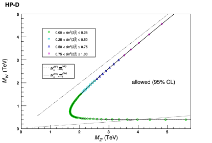
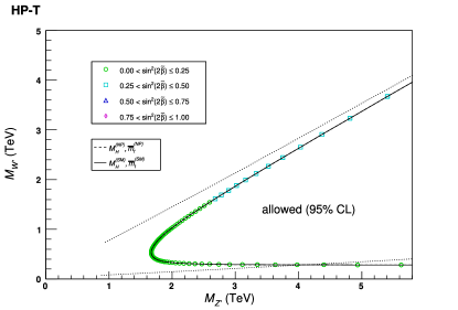
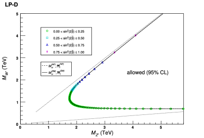
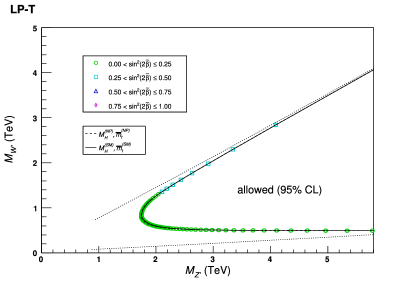
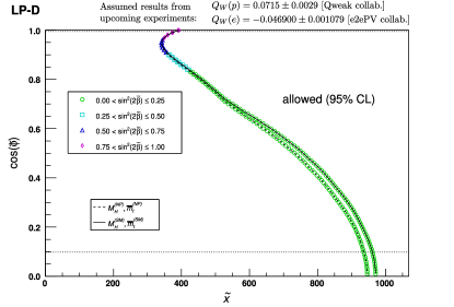
In this section, we present the allowed regions of parameter space based on the global-fit analysis. A testament to the success of the SM is that, for all the $G(221)$ models, the global fitting pushes $\tilde{x}$ to large values, decoupling the effects of the new physics. This is presented in Figs. 1 and 2, where we show the 95% confidence level (C.L.) contours on the $\tilde{x}-c_{\tilde{\phi}}$ plane.

Figure 1: The 95% confidence contours of the various models on the $\tilde{x}$-$\cos\phi$ plane, with $M_{H}$ and $\overline{m}_{t}$ either fixed as SM best-fit values (solid) or allowed to be re-fitted (dashed). The area to the right of each curve (large $\tilde{x}$ value) is allowed by the global-fit analysis.

Figure 2: Same as Fig. 1, but for the models that follow the breaking pattern II. The solid and dashed lines are almost indistinguishable.

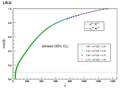
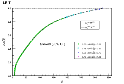
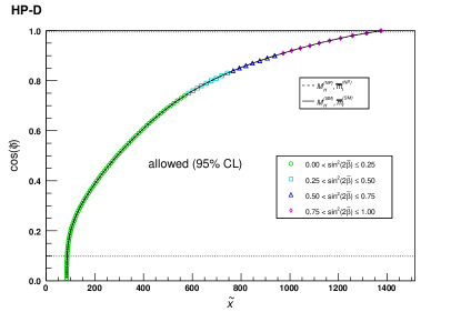
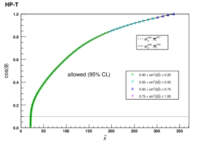
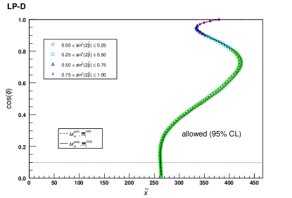
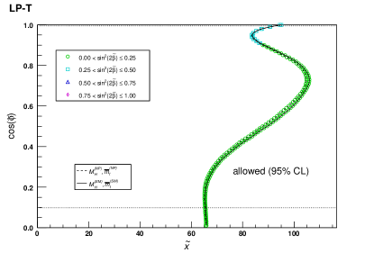
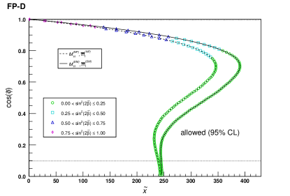
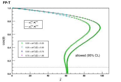
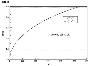
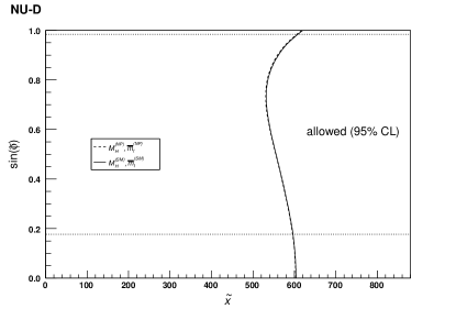
In addition to the constraints from the precision and low-energy data, we also require $\cos\phi$ ($\sin\phi$) to be greater than 0.1 (0.18) for the first (second) breaking pattern so that all the gauge couplings in Eq. (6), (7) and (8) are perturbative and do not exceed $\sqrt{4\pi}$. These constraints are shown as horizontal dotted lines in the figures.

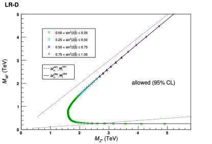
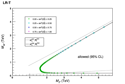
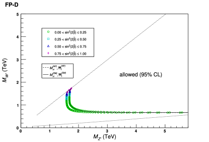
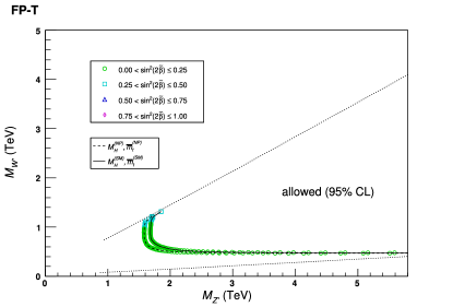
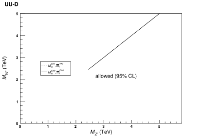
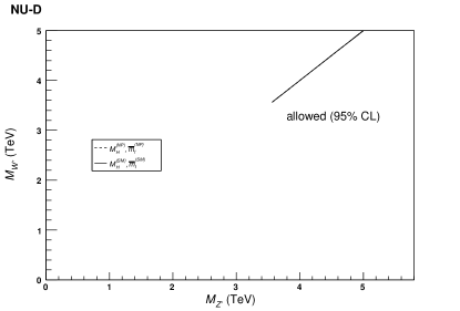
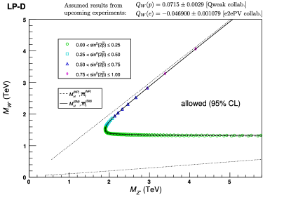
Since $\tilde{x}$ and $\tilde{\phi}$ are defined in a model-dependent manner, it is also useful to show the corresponding contours on the $M_{Z^{\prime}}$-$M_{W^{\prime}}$ plane to compare different $G(221)$ models. We translate the constraints on the parameter space of $\tilde{x}$ and $\tilde{\phi}$ to constraints on the masses of the new heavy gauge bosons, and plot these bounds on the $M_{Z^{\prime}}$-$M_{W^{\prime}}$ plane in Figs. 3 and 4. From these plots, we can read off the lower bounds on the masses of the $Z^{\prime}$ and the $W^{\prime}$ in these models, which are presented in Table 7. In the UU-D and the NU-D models, the masses of the $Z^{\prime}$ and the $W^{\prime}$ bosons are nearly degenerate, as shown in Fig. 4. In these two models, the minimum masses of the $Z^{\prime}$ and the $W^{\prime}$ consistent with the current experimental data are respectively $2.48~{}\mbox{TeV}$ and $3.56~{}\mbox{TeV}$.

Table 7: Lower bounds on the masses of the new heavy gauge bosons. The superscripts SM or NP indicate whether $M_{H}$ and $\bar{m}_{t}$ were set to their SM best-fit values or fitted with rest of new physics parameters. Compare with the plots of the $M_{Z^{\prime}}$–$M_{W^{\prime}}$ plane in Fig. 3.

	$M_{Z^{\prime}}^{\mbox{\tiny(SM)}}$ [TeV]	$M_{Z^{\prime}}^{\mbox{\tiny(NP)}}$ [TeV]	$M_{W^{\prime}}^{\mbox{\tiny(SM)}}$ [TeV]	$M_{W^{\prime}}^{\mbox{\tiny(NP)}}$ [TeV]
LR-D	1.602	1.602	0.269	0.269
LP-D	1.752	1.742	0.697	0.695
HP-D	1.674	1.673	0.403	0.403
FP-D	1.685	1.583	0.673	0.665
LR-T	1.607	1.607	0.197	0.197
LP-T	1.753	1.745	0.495	0.493
HP-T	1.680	1.679	0.289	0.289
FP-T	1.687	1.587	0.478	0.472
UU-D	2.479	2.474	2.479	2.474
NU-D	3.562	3.558	3.562	3.558

Figure 3: The 95% confidence contours of the various models on the $M_{Z^{\prime}}$-$M_{W^{\prime}}$ plane, with $M_{H}$ and $\overline{m}_{t}$ either fixed as SM best-fit values (solid) or allowed to be re-fitted (dashed). The dotted lines represent lines of constant $\cos\phi$ and $\sin\phi$ at fixed values of 0.1 (0.18) for the first (second) breaking pattern. Outside the cone surrounded by these regions, one of the gauge couplings becomes non-perturbative.

Figure 4: Same as Fig. 3, but for the models that follow the breaking pattern II. The contours appear as lines because in these models, $Z^{\prime}$ and $W^{\prime}$ are highly degenerate due to the pattern of symmetry breaking.

V.2 Key Observables and Their Impacts

For the models that follow the first pattern of symmetry breaking, we see that models in which Higgs triplets break $SU(2)_{2}\times U(1)_{X}$ lead to smaller bounds on $\tilde{x}$ compared to models where Higgs doublets break the symmetry. This is not surprising given Eqs. (54),(59) , where we see that, in the triplet models, the corrections to the definitions of the reference parameters are suppressed compared to the doublet models. However, the bounds on $M_{W^{\prime}}$ and $M_{Z^{\prime}}$ are comparable.

According to how the contours in parameter space are shaped, the considered $G(221)$ models can be separated into three classes:

• In the LR, HP, and UU models, large values of $c_{\tilde{\phi}}$ ($s_{\tilde{\phi}}$ for UU) are ruled out at small $\tilde{x}$. At small $c_{\tilde{\phi}}$ ($s_{\tilde{\phi}}$), the parameter contours, however, extend to relatively low $\tilde{x}$ values.

• The contours of the LP and FP models are, by contrast, located at comparatively larger $\tilde{x}$ values for small $c_{\tilde{\phi}}$. Increasing the values of $c_{\tilde{\phi}}$ to about 0.8, the contours of these models curve to the right (towards higher $\tilde{x}$). However, increasing $c_{\tilde{\phi}}$ further beyond about 0.8, the FP contours bend towards lower $\tilde{x}$, while the LP contours towards higher $\tilde{x}$.

• The parameter contour of the NU model is unique as it is the only curve that bends to the left with smaller $\tilde{x}$ value when going up along the vertical axis with increasing $s_{\tilde{\phi}}$ value.

The similarities and differences between the parameter plots can be traced back to certain key observables. That is, in the excluded regions of parameter spaces we consistently observe a pattern that several key observables contribute with especially large pulls to $\chi^{2}$, and it is these observables that drive the overall shapes of the curves in Fig. 1.

Table 8: Overview of the observables that drive the parameter plots. The most and second most important observables are respectively marked with the symbols ➀ and ➁. In the UU-D and NU-D models only one observable significantly contributes to $\chi^{2}$.

Model	$\sigma_{\mbox{\tiny had}}$	$A_{FB}(b)$	$\left(g_{\mbox{\tiny{$L$}}}^{\mbox{\tiny{$\nu N$}}}\right)^{2}$	$Q_{W}({}^{133}\mbox{Cs})$	Set of other obs.
LR, HP	➀	➁
LP, FP			➁	➀
UU	➀				➁
NU			➀		➁

In Table 8 we give an overview of these observables that effectively drive the results in Fig. 1. For each model in the breaking pattern I, we list the two most important observables. For the models of the breaking pattern II, we give only one such observable. It is important to note that Table 8 only presents qualitative observations that indicate tendencies, and it may be the case that some particular points of the parameter spaces have other observables that contribute with larger pulls than the ones we indicate here. Nevertheless, the patterns we give here are useful in indicating qualitatively which observables are likely to be sensitive to new physics contributions from the $G(221)$ models.

The explicit expressions for the new physics corrections to these key observables, are listed in Tables 9 and 10. At the $95\%$ C.L., the set of observables ($\sigma_{\mbox{\tiny had}}$, $A_{FB}(b)$, $A_{LR}(e)$, $\left(g_{\mbox{\tiny{$L$}}}^{\mbox{\tiny{$\nu N$}}}\right)^{2}$, $Q_{W}({}^{133}\mbox{Cs})$) is respectively measured with a precision at the ($0.18,3.16,2.80,0.90,1.24$) percent level.

Table 9: Fractional new physics corrections to the observables $\sigma_{\mbox{\tiny had}}$, $A_{FB}(b)$ and $Q_{W}\left({}^{133}\mbox{Cs}\right)$ relative to the corresponding SM predictions. To obtain the new physics shifts in the triplet versions of the LR, LP, HP and FP models, the prefactors of $s_{2\tilde{\beta}}^{2}$ need to be multiplied by $\frac{1}{2}$, all other terms by $\frac{1}{4}$.

	$\tilde{x}\ \delta\sigma_{\mbox{\tiny had}}/\sigma_{\mbox{\tiny had,SM}}$	$\tilde{x}\ \delta A_{FB}(b)/A_{FB,\mbox{\tiny SM}}(b)$
LR-D	$-1.13\ c_{\tilde{\phi}}^{2}-0.142\ c_{\tilde{\phi}}^{4}+0.0432\ s_{2\tilde{\beta}}^{2}$	$-30.0\ c_{\tilde{\phi}}^{2}+67.6\ c_{\tilde{\phi}}^{4}-20.6\ s_{2\tilde{\beta}}^{2}$
LP-D	$+0.346\ c_{\tilde{\phi}}^{2}-0.142\ c_{\tilde{\phi}}^{4}+0.0432\ s_{2\tilde{\beta}}^{2}$	$-46.1\ c_{\tilde{\phi}}^{2}+67.6\ c_{\tilde{\phi}}^{4}-20.6\ s_{2\tilde{\beta}}^{2}$
HP-D	$-1.38\ c_{\tilde{\phi}}^{2}-0.142\ c_{\tilde{\phi}}^{4}+0.0432\ s_{2\tilde{\beta}}^{2}$	$-30.9\ c_{\tilde{\phi}}^{2}+67.6\ c_{\tilde{\phi}}^{4}-20.6\ s_{2\tilde{\beta}}^{2}$
FP-D	$+0.0985\ c_{\tilde{\phi}}^{2}-0.142\ c_{\tilde{\phi}}^{4}+0.0432\ s_{2\tilde{\beta}}^{2}$	$-47.0\ c_{\tilde{\phi}}^{2}+67.6\ c_{\tilde{\phi}}^{4}-20.6\ s_{2\tilde{\beta}}^{2}$
UU	$-0.889\ s_{\tilde{\phi}}^{2}-0.0132\ s_{\tilde{\phi}}^{4}$	$+0.161\ s_{\tilde{\phi}}^{2}+6.29\ s_{\tilde{\phi}}^{4}$
NU	$+0.583\ s_{\tilde{\phi}}^{2}-0.0132\ s_{\tilde{\phi}}^{4}$	$+14.2\ s_{\tilde{\phi}}^{2}+6.29\ s_{\tilde{\phi}}^{4}$

	$\tilde{x}\ \delta Q_{W}\left({}^{133}\mbox{Cs}\right)/Q_{W,\mbox{\tiny SM}}\left({}^{133}\mbox{Cs}\right)$
LR-D	$-0.855\ c_{\tilde{\phi}}^{4}-0.145\ s_{2\tilde{\beta}}^{2}$
LP-D	$+3.35-1.95\ c_{\tilde{\phi}}^{2}-0.855\ c_{\tilde{\phi}}^{4}-0.145\ s_{2\tilde{\beta}}^{2}$
HP-D	$-0.855\ c_{\tilde{\phi}}^{4}-0.145\ s_{2\tilde{\beta}}^{2}$
FP-D	$+2.95-1.95\ c_{\tilde{\phi}}^{2}-0.855\ c_{\tilde{\phi}}^{4}-0.145\ s_{2\tilde{\beta}}^{2}$
UU	$-0.855\ s_{\tilde{\phi}}^{4}$
NU	$+0.406+0.594\ s_{\tilde{\phi}}^{2}-0.855\ s_{\tilde{\phi}}^{4}$

Table 10: New physics corrections to the observable $\left(g_{\mbox{\tiny{$L$}}}^{\mbox{\tiny{$\nu N$}}}\right)^{2}$ relative to the prediction of the SM.

	$\tilde{x}\ \delta\left(g_{\mbox{\tiny{$L$}}}^{\mbox{\tiny{$\nu N$}}}\right)^{2}/\left(g_{\mbox{\tiny{$L$}},\mbox{\tiny SM}}^{\mbox{\tiny{$\nu N$}}}\right)^{2}$
LR-D, LP-D, HP-D, FP-D	$0.0875+1.91\ c_{\tilde{\phi}}^{2}+0.839\ c_{\tilde{\phi}}^{4}-2.84\ s_{2\tilde{\beta}}^{2}$
LR-T, LP-T, HP-T, FP-T	$0.0219+0.478\ c_{\tilde{\phi}}^{2}+0.210\ c_{\tilde{\phi}}^{4}-1.42\ s_{2\tilde{\beta}}^{2}$
UU-D	$0.839\ s_{\tilde{\phi}}^{4}$
NU-D	$2.58-0.583\ s_{\tilde{\phi}}^{2}+0.839\ s_{\tilde{\phi}}^{4}$

Based on these expressions we can roughly reconstruct the respective shapes of the contours, and in Fig. 5 we illustrate our argumentation.

Figure 5: Sketches illustrating the influences of some key observables on the parameter bounds for the models of the first breaking pattern. The UU-D parameter contour is driven by $\sigma_{\mbox{\tiny had}}$ as well. In the NU-D model $\left(g_{\mbox{\tiny{$L$}}}^{\mbox{\tiny{$\nu N$}}}\right)^{2}$ is the most important observable.

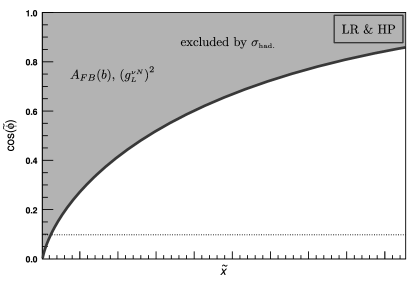
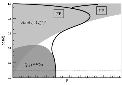
We find that the shapes of the contours for LR, HP and UU models are driven by $\sigma_{\mbox{\tiny had}}$. For the LR and HP models, $A_{FB}(b)$ and $A_{LR}(e)$ also play an important role. Since $A_{FB}(b)$ is defined as $A_{FB}(b)\equiv\frac{3}{4}A_{LR}(e)A_{FB}(b)$, the large coefficients in $x\delta A_{FB}^{b}/A_{FB}^{b}$ (See Table 9) originate from the smallness of the SM value of $A_{LR}^{e}$. The combination $x\delta A_{FB}^{b}/A_{FB}^{b}$ imposes about the same constraints as those derived from $x\delta A_{LR}^{e}/A_{LR}^{e}$. Since they are strongly correlated, we only list the observable $A_{FB}(b)$. In the LP and FP models, with low $c_{\tilde{\phi}}$ values, $Q_{W}\left({}^{133}\mbox{Cs}\right)$ is the most important observable, because of the large constant terms independent of $\tilde{\phi}$ or $\tilde{\beta}$ in $Q_{W}$, as shown in Table 9. The constant term for either the LR-D or the HP-D model vanishes because it is proportional to $(T_{L}^{3}-T^{3}_{R})$ of the electron with the quantum number assignment $T_{L}^{3}=T^{3}_{R}=-1/2$. With high $c_{\tilde{\phi}}$ values, the observable $\left(g_{\mbox{\tiny{$L$}}}^{\mbox{\tiny{$\nu N$}}}\right)^{2}$ determines the shape of the parameter contours. The NU contour is mainly driven by the pull of $\left(g_{\mbox{\tiny{$L$}}}^{\mbox{\tiny{$\nu N$}}}\right)^{2}$. ( We note that, $A_{FB}(b)$ has a similar effect on the LP and FP contours as on the LR and HP contours, though subdominant compared to the other observables. The same applies to $\left(g_{\mbox{\tiny{$L$}}}^{\mbox{\tiny{$\nu N$}}}\right)^{2}$ for the LR and HP models.)

The starting point of our discussion is that the SM represents the best description of the present experimental data, and the $G(221)$ parameters have to be chosen such that they minimize the new physics shifts. We first focus on models in the breaking pattern I, the LR, LP, HP, and FP models, and note the following points:

• The observables $A_{FB}(b)$ and $\left(g_{\mbox{\tiny{$L$}}}^{\mbox{\tiny{$\nu N$}}}\right)^{2}$ prefer small $c_{\tilde{\phi}}$. In $\delta\left(g_{\mbox{\tiny{$L$}}}^{\mbox{\tiny{$\nu N$}}}\right)^{2}$, the $c_{\tilde{\phi}}^{2}$ and $c_{\tilde{\phi}}^{4}$ terms have the same sign so that they cannot cancel each other. $A_{FB}(b)$ has the largest effect on the allowed parameter space in the LR and HP models as the coefficients of $c_{\tilde{\phi}}^{2}$ and $c_{\phi}^{4}$ are large in magnitude.

• In the case of the LR and HP models the $c_{\tilde{\phi}}^{2}$ and $c_{\tilde{\phi}}^{4}$ contributions to $\delta\sigma_{\mbox{\tiny had}}$ have the same sign and the $s_{2\tilde{\beta}}^{2}$ term is suppressed by a small prefactor. The pull of $\sigma_{\mbox{\tiny had}}$ therefore represents the hindrance for the LR and HP models to accommodate large values of $c_{\tilde{\phi}}$ at smaller $\tilde{x}$.

• The large impact of $Q_{W}\left({}^{133}\mbox{Cs}\right)$ on the LP and FP bounds is due to the large constant term in $\delta Q_{W}\left({}^{133}\mbox{Cs}\right)$. The only way to make $\delta Q_{W}\left({}^{133}\mbox{Cs}\right)$ small (other than simply raising $\tilde{x}$) is to have large $c_{\tilde{\phi}}$ so that the negative contributions from the $c_{\tilde{\phi}}^{2}$ and $c_{\tilde{\phi}}^{4}$ terms can compete with the positive constant term. Consequently, the low-$c_{\tilde{\phi}}$ region is ruled out in the LP and FP models and the parameter contours start at higher $\tilde{x}$ values than in the LR and HP models.

• In the $\sigma_{had.}$, $A_{FB}(b)$ and $(g^{\nu N}_{L})^{2}$ observables, the $s_{2\tilde{\beta}}^{2}$ and $c_{\tilde{\phi}}^{4}$ terms always have opposite sign. The LP and FP parameter plots suggest that, depending on the exact interplay between $s_{2\tilde{\beta}}^{2}$ and $c_{\tilde{\phi}}$, the $s_{2\tilde{\beta}}^{2}$ terms may be able to overcome the $c_{\tilde{\phi}}^{4}$ contributions such that the contours are pulled back towards lower $\tilde{x}$ values. Note, however, that the expressions given in Table 9 cannot explain the branching between the LP and FP contours. To account for that effect we certainly would have to extend our discussion to a larger set of observables.

After these comments on the models of the breaking pattern I, it is easy to understand the shape of the UU and NU contours. In the UU model all shifts that we present in Tables 9 and 10 favor small $s_{\tilde{\phi}}$ values. Especially the fact that the $s_{\tilde{\phi}}^{2}$ and $s_{\tilde{\phi}}^{4}$ terms in $\delta\sigma_{\mbox{\tiny had}}$ have the same sign leads to the exclusion of the high-$s_{\tilde{\phi}}$ region. For that reason the UU plot looks similar to the plots of the LR and HP models. The contour of the NU-D model is mainly influenced by the correction to $\left(g_{\mbox{\tiny{$L$}}}^{\mbox{\tiny{$\nu N$}}}\right)^{2}$. Since $\delta\left(g_{\mbox{\tiny{$L$}}}^{\mbox{\tiny{$\nu N$}}}\right)^{2}$ is small if $s_{\tilde{\phi}}$ takes some intermediate value we observe a bump in the NU-D contour towards lower $\tilde{x}$ values for $s_{\tilde{\phi}}$ values around $0.7$.

An important consequence of identifying these observables is that we may anticipate the future impact that the upcoming measurements, with greater precision, may have on the global analysis. For example, the Q-weak collaboration VanOers:2007zz and the e2ePV collaboration Mack:2006 at Jefferson Lab are expected to have ultra-high precision measurements of the weak charge of the proton $Q_{W}(p)$ and the electron $Q_{W}(e)$ (with a fractional uncertainties of respectively 4% and 2.5%). As $Q_{W}(\ ^{133}\mbox{Cs})$ is a key observable in driving the results for the lepto-phobic (LP) and fermio-phobic (FP) models, we would expect that the future measurements of $Q_{W}(e)$ and $Q_{W}(p)$ would have a great impact on the global-fit analysis. This is demonstrated in Fig. 6, where we perform the global-fit analysis with the expected future uncertainty of $Q_{W}(p)$ and $Q_{W}(e)$. We find that the LP-D contour is drastically different than those presented in Fig. 1. As a result of these further constraints from the $Q_{W}(p)$ and $Q_{W}(e)$, the allowed region in the $M_{Z^{\prime}}-M_{W^{\prime}}$ plane shrinks as well. The lower bounds for the $W^{\prime}$ mass increase, for instance in LP-D model, from about $0.7~{}\mbox{TeV}$ to $1.3\ \mbox{TeV}$.

Figure 6: The $\tilde{x}-\cos(\tilde{\phi})$ and $M_{Z^{\prime}}$-$M_{W^{\prime}}$ contours for the LP-D model with an expected uncertainty in the Q-weak data and the e2ePV data. These plots should be compared with the corresponding plots in Figs. 1 and 3,and demonstrate that, since $Q_{W}(e)$ is a key observable for the LP model, an increase of precision in its measurement has a large impact on the global analysis. In particular, at low $c_{\tilde{\phi}}$, the lower bound on $\tilde{x}$ is substantially increased.

V.3 Constraints from Triple Gauge Boson Couplings

Though we do not include the shifts to the triple gauge boson couplings (TGC) in our global analysis, they are nonetheless precise measurements at LEP-II that can be used to constrain models of new physics. In particular, the $ZWW$ vertex is measured to a precision of about 2% and may be used to constrain models of new physics Amsler:2008zzb . In this subsection, we compute the shift to the $ZWW$ vertex, and use it as a complementary constraint when we discuss the results of our global analysis.

The shift in the $ZWW$ vertex can be parameterized by the Hagiwara’s parameterization Hagiwara:1986vm

$$g_{\mbox{\tiny ZWW}}=g^{\mbox{\tiny SM}}_{\mbox{\tiny ZWW}}\left(g_{1}^{Z}\right),$$ (106)

where the SM value of $g_{1}^{Z}$ is unity. At LEP-II, using a partial waves analysis, the measured $ZWW$ vertex is Schael:2004tq

$$g_{1}^{Z}=1.001\pm 0.027\pm 0.013,$$ (107)

where the uncertainties are respectively the 1$\sigma$ statistical and systematic uncertainties. Adding these uncertainties in quadrature, we have

$$g_{1}^{Z}=1.001\pm 0.030.$$ (108)

It is important to note, however, that the measurement of the $ZWW$ vertex is extracted from the process $e^{+}e^{-}\rightarrow W^{+}W^{-}$ using an event shape analysis (including angular distributions) assuming SM couplings for all other vertices. Thus, to properly use the experimental results, we have to compute the entire $e^{+}e^{-}\rightarrow W^{+}W^{-}$ amplitude and attribute all the shifts in the amplitude to $\Delta g_{1}^{Z}$.

The full amplitude of the tree-level process $e^{+}e^{-}\rightarrow W^{+}W^{-}$ is the sum of three diagrams: $s$-channel $\gamma$-exchange, $s$-channel $Z$-exchange, and $t$-channel $\nu$-exchange. We denote these three amplitudes respectively as $\mathcal{A}_{\gamma}$, $\mathcal{A}_{Z}$, and $\mathcal{A}_{\nu}$. Even though the LEP experiments utilize unpolarized $e^{\pm}$ beams, it is useful to consider amplitudes with specific helicities for both $e^{\pm}$ and $W^{\pm}$ and employ the helicity amplitude method Xu:1986xb to analyze the amplitudes. The individual amplitudes are computed in Hagiwara et al. Hagiwara:1986vm , and here we only note the key features of the dependence in the polar angle $\theta$. For a given configuration of incoming and outgoing particle helicities, all three amplitudes $\mathcal{A}_{\gamma,Z,\nu}$ are proportional to the Wigner’s $d$- matrix elements. For the $s$-channel amplitudes, this is the only dependence in the scattering angle $\theta$ (not to be confused with the weak mixing angle)

$$\mathcal{A}_{\gamma,Z}\propto d^{\Delta\sigma,\Delta\lambda}_{\Delta J}(\theta).$$ (109)

For the $t$-channel, $\nu$-exchange, we have additional $\theta$ dependence from the $\nu$-propagator

$$\mathcal{A}_{\nu}\propto\left(B-\frac{C}{1+\beta^{2}-2\beta\cos\theta}\right)d^{\Delta\sigma,\Delta\lambda}_{\Delta J}(\theta),$$ (110)

where $B$ and $C$ depend on the helicity configuration, but are independent of $\theta$. Thus, for a fixed helicity configuration of $e^{+}e^{-}\rightarrow W^{+}W^{-}$, we can perform a partial wave analysis to project out the $d^{\Delta\sigma,\Delta\lambda}_{\Delta J}(\theta)$ component of the amplitudes

$$\tilde{\mathcal{A}}_{\gamma,Z,\nu}\equiv\int\limits_{0}^{\pi}\mathcal{A}_{\gamma,Z,\nu}d^{\Delta\sigma,\Delta\lambda}_{\Delta J}(\theta)d(\cos\theta)$$ (111)

The uncertainties in $g_{1}^{Z}$ (which we denote as $\Delta g_{Z}^{1}$) can be used to constrain the $G(221)$ models by first identifying

$$\tilde{\mathcal{A}}_{\gamma}^{G(221)}+\tilde{\mathcal{A}}_{Z}^{G(221)}+\tilde{\mathcal{A}}_{\nu}^{G(221)}=\tilde{\mathcal{A}}_{\gamma}^{\mbox{\scriptsize SM}}+\left(1+\Delta g_{1}^{Z}\right)\tilde{\mathcal{A}}_{Z}^{\mbox{\scriptsize SM}}+\tilde{\mathcal{A}}_{\nu}^{\mbox{\scriptsize SM}},$$ (112)

and then express each amplitude in the $G(221)$ model in terms of the reference and fit parameters

$$\tilde{\mathcal{A}}_{\gamma,Z,\nu}^{G(221)}=\tilde{\mathcal{A}}_{\gamma,Z,\nu}^{\mbox{\scriptsize SM}}\left(1+\frac{1}{\tilde{x}}\delta\tilde{\mathcal{A}}_{\gamma,Z,\nu}\right),$$ (113)

where the fractional shifts in the amplitudes $\delta\tilde{\mathcal{A}}_{\gamma,Z,\nu}$ are functions of $\tilde{\phi}$ and $\tilde{\beta}$. For a fixed helicity configuration of $e^{+}e^{-}\rightarrow W^{+}W^{-}$, we can compute $\tilde{\mathcal{A}}_{\gamma,Z,\nu}$ for both the SM and $G(221)$ models and obtain an excluded region on the $\tilde{x}$-$\cos\phi$ plane. The regions that are allowed by all the helicity combinations are shown in Fig. 7.

Figure 7: The regions on the $\tilde{x}$-$\cos\phi$ plane excluded by experimental measurements of $\Delta g_{1}^{Z}$ (in grey) for models in the breaking pattern I, for the cases $\sin^{2}2\tilde{\beta}=0$ and $1$.

We note that, generally, the bounds given by $\Delta g_{1}^{Z}$ are more relaxing than those obtained from the global-fit analysis earlier. In fact, for small values of $\tilde{\beta}$, the regions excluded by $\Delta g_{1}^{Z}$ are already excluded by the global-fit analysis presented in the previous subsection.

VI Conclusions

In this work we analyze the constraints on the masses of the heavy gauge bosons of the $G(221)$ (including the left-right (LR), leptophobic (LP), hadrophobic (HP) and fermiophobic (FP) as well as the ununified (UU) and non-universal (NU)) models in a unified view based on the classification of the $G(221)$ models in terms of the patterns of symmetry breaking and the gauge couplings of fermions. Adapting the framework of effective field theory, we give the effective Lagrangians at the electroweak scale and low energy scale , applicable to any $G(221)$ model, and perform a global-fit analysis about a set of $37$ electroweak observables, including $Z$ pole data, the mass and the width of the $W^{\pm}$ boson, and various low-energy observables. The experimental precision with which these observables have been measured allows us to put strong bounds on the parameter space of the $G(221)$ models and to constrain the masses of the $Z^{\prime}$ and $W^{\prime\pm}$ bosons. At the same time, we show that the bounds from the triple gauge boson couplings on the parameters do not affect the result of the global-fit analysis. We present our key results in terms of 95% C.L. contours of the allowed regions both on the $\tilde{x}$-$\cos\tilde{\phi}$ plane, as well as on the $M_{Z^{\prime}}$-$M_{W^{\prime}}$ plane, from which we can readily give the lower bounds on the masses of the $W^{\prime}$ and $Z^{\prime}$, which are presented in Table 7, which can be used as a guide for future collider search. We show that, in the first breaking pattern, although the mass of $Z^{\prime}$ is about $1.7$ TeV, the mass of the $W^{\prime}$ in some models can be relatively light (of a few hundreds of GeV), particularly in the left-right (LR), hadrophobic (HP) models. In the case of the second breaking pattern, due the near-degeneracy between the masses of the $Z^{\prime}$ and the $W^{\prime\pm}$, the $W^{\prime}$ is necessarily heavy.

In addition to the constraints on the parameters and bounds on the extra gauge boson masses, we also find associations between certain key observables and the $G(221)$ models discussed in this paper. As these observables are responsible for ‘driving’ the shape of the 95% contour plots, future measurements on these particular observables would have a tremendous impact on our results. We demonstrate such an example in Fig. 6, showing that an anticipated precision on the measurement of $Q_{W}(e)$ could largely increase the lower bound on the $W^{\prime}$ mass from the current value of $0.7~{}\mbox{TeV}$ to $1.3\ \mbox{TeV}$ in the LP-D model.

In this work, we focus on the interactions of the heavy $W^{\prime}$ and $Z^{\prime}$ bosons to fermions. To extend our results to include flavor-dependent observables, such as the branching ratio $\mbox{Br}(b\rightarrow s\gamma)$ and the anomalous magnetic moment of the muon, requires a detailed specification of the flavor sectors of the $G(221)$ models. Though it is difficult to enumerate the many models in the literature, in the advent of the Large Hadron Collider (LHC), it would be useful to extend to the flavor sector the insights provided in this work. Moreover, the direct search of the $W^{\prime}$ and $Z^{\prime}$ bosons at the Fermilab Tevatron could further constrain the $G(221)$ model parameter space. The potential of the Tevatron and LHC to observe the $W^{\prime}$ and $Z^{\prime}$ bosons will be presented in a separate work.

Appendix A Effective Lagrangians

In this appendix we show how to obtain the coulping coefficients in the effective Lagrangian. There are two effective Lagrangians in our framework. The first effective Lagrangian is SM-like, and is applicable at the electroweak scale after integrating out $Z^{\prime}$ and $W^{\prime}$, we parameterize this Lagrangian as

$$\mathcal{L}_{\mbox{\tiny eff}}^{\mbox{\tiny ew}} =g^{\mbox{\tiny L}}_{Z\overline{f}f}Z_{\mu}\overline{f}\gamma^{\mu}P_{\mbox{\tiny L}}f+g^{\mbox{\tiny R}}_{Z\overline{f}f}Z_{\mu}\overline{f}\gamma^{\mu}P_{\mbox{\tiny R}}f+\left(g^{\mbox{\tiny L}}_{W\overline{f_{1}}f_{2}}W^{+}_{\mu}\overline{f}_{1}\gamma^{\mu}P_{\mbox{\tiny L}}f_{2}+g^{\mbox{\tiny R}}_{W\overline{f_{1}}f_{2}}W^{+}_{\mu}\overline{f}_{1}\gamma^{\mu}P_{\mbox{\tiny R}}f_{2}+\mbox{h.c.}\right)$$

$$-B\left(\left(\overline{f}_{1}f_{2}\right)_{\mbox{\tiny L,R}},\left(\overline{f}_{3}f_{4}\right)_{\mbox{\tiny L,R}}\right)\frac{G_{F}}{\sqrt{2}}\left(\overline{f}_{1}f_{2}\right)_{\mbox{\tiny L,R}}\left(\overline{f}_{3}f_{4}\right)_{\mbox{\tiny L,R}}.$$ (114)

Except for the non-universal (NU) model, the couplings $g^{\mbox{\tiny L,R}}_{Z\overline{f}f}$, $g^{\mbox{\tiny L,R}}_{Z\overline{f}f}$ and $B\left(\left(\overline{f}_{1}f_{2}\right)_{\mbox{\tiny L,R}},\left(\overline{f}_{3}f_{4}\right)_{\mbox{\tiny L,R}}\right)$ are all flavor-universal. The second effective Lagrangian is Fermi’s theory of four-fermion interactions. It is obtained upon further integrating out $Z$ and $W$ bosons, and is applicable below the electroweak scale. We parameterize this Lagrangian as

$$\mathcal{L}_{\mbox{\tiny eff}}^{\mbox{\tiny 4-fermion}} =-C\left(\left(\overline{f}_{1}f_{2}\right)_{\mbox{\tiny L,R}},\left(\overline{f}_{3}f_{4}\right)_{\mbox{\tiny L,R}}\right)\frac{G_{F}}{\sqrt{2}}\left(\overline{f}_{1}f_{2}\right)_{\mbox{\tiny L,R}}\left(\overline{f}_{3}f_{4}\right)_{\mbox{\tiny L,R}}.$$ (115)

The above coefficient functions $g^{\mbox{\tiny L,R}}_{Z\overline{f}f}$, $g^{\mbox{\tiny L,R}}_{W\overline{f_{1}}f_{2}}$ and $C\left(\left(\overline{f}_{1}f_{2}\right)_{\mbox{\tiny L,R}},\left(\overline{f}_{3}f_{4}\right)_{\mbox{\tiny L,R}}\right)$ can be obtained by the following steps:

• write down the specific form of the effective Lagrangians at the electroweak scale and low energy scale by plugging the formulae in Tables 4 and 5 into the Eqs. (39) and (40);

• extract the coulpings $g^{\mbox{\tiny L,R}}_{Z\overline{f}f}$, $g^{\mbox{\tiny L,R}}_{W\overline{f_{1}}f_{2}}$ and $C$ by comparing the parametrized Lagrangians in Eqs. (114) and (115) with the specific form of the effective Lagrangians;

• replace all the model parameters $\tilde{e}$, $\tilde{v}$, and $\tilde{\theta}$ in the expressions of $g^{\mbox{\tiny L,R}}_{Z\overline{f}f}$, $g^{\mbox{\tiny L,R}}_{W\overline{f_{1}}f_{2}}$, and $C$ by reference parameters $\alpha$, $G_{F}$ and $M_{Z}$, using the relations in Eqs. (59), (58) and (60).

For future reference, we list below the coefficient functions $g^{\mbox{\tiny L,R}}_{Z\overline{f}f}$, $g^{\mbox{\tiny L,R}}_{W\overline{f_{1}}f_{2}}$ and $C\left(\left(\overline{f}_{1}f_{2}\right)_{\mbox{\tiny L,R}},\left(\overline{f}_{3}f_{4}\right)_{\mbox{\tiny L,R}}\right)$ in terms of the model parameters. We also give some examples of the final form of the coefficients in terms of the fit parameters.

A.1 The LR-D, LP-D, HP-D, and FP-D Models

For the four models that follow the first breaking pattern with a doublet (LR-D, LP-D, HP-D, and FP-D models), the difference in the coefficient functions is originated from the quantum numbers of the fermions. In Table 11, we give the quantum numbers of the fermions, and present the coefficients of the effective Lagrangian in terms of these quantum numbers.

Table 11: The charge assignments of the SM fermions for the first breaking patter. $T_{3L}^{f}$ and $T_{3R}^{f}$ are respectively the third component of the isospin for the $SU(2)_{1}$ and $SU(2)_{2}$ gauge groups (which are conventionally called $SU(2)_{L}$ and $SU(2)_{R}$ in left-right models). These charge assignments apply to all three generations.

		$T_{L}^{3}$	$T_{R}^{3}$	$X^{f}$			$T_{L}^{3}$	$T_{R}^{3}$	$X^{f}$			$T_{L}^{3}$	$T_{R}^{3}$	$X^{f}$			$T_{L}^{3}$	$T_{R}^{3}$	$X^{f}$
LR	$\nu_{\mbox{\tiny L}}$	$+\tfrac{1}{2}$	0	$-\tfrac{1}{2}$	LP	$\nu_{\mbox{\tiny L}}$	$+\tfrac{1}{2}$	0	$-\tfrac{1}{2}$	HP	$\nu_{\mbox{\tiny L}}$	$+\tfrac{1}{2}$	0	$-\tfrac{1}{2}$	FP	$\nu_{\mbox{\tiny L}}$	$+\tfrac{1}{2}$	0	$-\tfrac{1}{2}$
	$e_{\mbox{\tiny L}}$	$-\tfrac{1}{2}$	0	$-\tfrac{1}{2}$		$e_{\mbox{\tiny L}}$	$-\tfrac{1}{2}$	0	$-\tfrac{1}{2}$		$e_{\mbox{\tiny L}}$	$-\tfrac{1}{2}$	0	$-\tfrac{1}{2}$		$e_{\mbox{\tiny L}}$	$-\tfrac{1}{2}$	0	$-\tfrac{1}{2}$
	$u_{\mbox{\tiny L}}$	$+\tfrac{1}{2}$	0	$+\tfrac{1}{6}$		$u_{\mbox{\tiny L}}$	$+\tfrac{1}{2}$	0	$+\tfrac{1}{6}$		$u_{\mbox{\tiny L}}$	$+\tfrac{1}{2}$	0	$+\tfrac{1}{6}$		$u_{\mbox{\tiny L}}$	$+\tfrac{1}{2}$	0	$+\tfrac{1}{6}$
	$d_{\mbox{\tiny L}}$	$-\tfrac{1}{2}$	0	$+\tfrac{1}{6}$		$d_{\mbox{\tiny L}}$	$-\tfrac{1}{2}$	0	$+\tfrac{1}{6}$		$d_{\mbox{\tiny L}}$	$-\tfrac{1}{2}$	0	$+\tfrac{1}{6}$		$d_{\mbox{\tiny L}}$	$-\tfrac{1}{2}$	0	$+\tfrac{1}{6}$
	$\nu_{\mbox{\tiny R}}$	$0$	$+\tfrac{1}{2}$	$-\tfrac{1}{2}$		$\nu_{\mbox{\tiny R}}$	$0$	$0$	$0$		$\nu_{\mbox{\tiny R}}$	$0$	$+\tfrac{1}{2}$	$-\tfrac{1}{2}$		$\nu_{\mbox{\tiny R}}$	$0$	$0$	$0$
	$e_{\mbox{\tiny R}}$	$0$	$-\tfrac{1}{2}$	$-\tfrac{1}{2}$		$e_{\mbox{\tiny R}}$	$0$	$0$	$-1$		$e_{\mbox{\tiny R}}$	$0$	$-\tfrac{1}{2}$	$-\tfrac{1}{2}$		$e_{\mbox{\tiny R}}$	$0$	$0$	$-1$
	$u_{\mbox{\tiny R}}$	$0$	$-\tfrac{1}{2}$	$+\tfrac{1}{6}$		$u_{\mbox{\tiny R}}$	$0$	$-\tfrac{1}{2}$	$+\tfrac{1}{6}$		$u_{\mbox{\tiny R}}$	$0$	$0$	$+\tfrac{2}{3}$		$u_{\mbox{\tiny R}}$	$0$	$0$	$+\tfrac{2}{3}$
	$d_{\mbox{\tiny R}}$	$0$	$-\tfrac{1}{2}$	$+\tfrac{1}{6}$		$d_{\mbox{\tiny R}}$	$0$	$-\tfrac{1}{2}$	$+\tfrac{1}{6}$		$d_{\mbox{\tiny R}}$	$0$	$0$	$-\tfrac{1}{3}$		$d_{\mbox{\tiny R}}$	$0$	$0$	$-\tfrac{1}{3}$

Performing the above procedure, we obtain

$$g^{\mbox{\tiny L}}_{W\overline{f_{1}}f_{2}} =\frac{\mbox{$\tilde{e}$}}{\mbox{$\sqrt{2}s_{\tilde{\theta}}$}},$$ (116)

$$g^{\mbox{\tiny R}}_{W\overline{f_{1}}f_{2}} =\begin{cases}\frac{\mbox{$\tilde{e}$}}{\mbox{$\sqrt{2}s_{\tilde{\theta}}$}}\frac{\mbox{$s_{2\tilde{\beta}}$}}{\mbox{$\tilde{x}$}},&\mbox{(for $f_{1,2}$ as quarks in LR and LP, and leptons in LR and HP)}\\ 0,&\mbox{(for $f_{1,2}$ as quarks in HP and FP, and leptons in LP and FP)}\end{cases}$$ (117)

$$g^{\mbox{\tiny L}}_{Z\overline{f}f} =\frac{\mbox{$\tilde{e}$}}{\mbox{$s_{\tilde{\theta}}c_{\tilde{\theta}}$}}\left(T^{3}_{L}-s_{\tilde{\theta}}^{2}Q+\frac{\mbox{$s_{\tilde{\phi}}^{2}c_{\tilde{\phi}}^{2}$}}{\mbox{$\tilde{x}$}}(T^{3}_{L}-Q)\right),$$ (118)

$$g^{\mbox{\tiny R}}_{Z\overline{f}f} =\frac{\mbox{$\tilde{e}$}}{\mbox{$s_{\tilde{\theta}}c_{\tilde{\theta}}$}}\left(-s_{\tilde{\theta}}^{2}Q+\frac{\mbox{$c_{\tilde{\phi}}^{2}$}}{\mbox{$\tilde{x}$}}(T^{3}_{R}-s_{\tilde{\phi}}^{2}Q)\right),$$ (119)

and the neutral-current four-fermion coupling coefficients

$$\frac{\mbox{$1$}}{\mbox{$2$}}C\left(\left(\overline{f}f\right)_{\mbox{\tiny L}},\left(\overline{f}^{\prime}f^{\prime}\right)_{\mbox{\tiny L}}\right) =(1+\frac{\mbox{$c_{\tilde{\phi}}^{4}$}}{\mbox{$\tilde{x}$}}-\frac{\mbox{$s_{2\tilde{\beta}}^{2}$}}{\mbox{$\tilde{x}$}})(T^{3}_{L}-s_{\tilde{\theta}}^{2}Q)(T^{\prime 3}_{L}-s_{\tilde{\theta}}^{2}Q^{\prime})$$

$$+\frac{\mbox{$s_{\tilde{\phi}}^{2}c_{\tilde{\phi}}^{2}$}}{\mbox{$\tilde{x}$}}\left[(T^{3}_{L}-s_{\tilde{\theta}}^{2}Q)(T^{\prime 3}_{L}-Q^{\prime})+(T^{3}_{L}-Q)(T^{\prime 3}_{L}-s_{\tilde{\theta}}^{2}Q^{\prime})\right]$$

$$+\frac{\mbox{$s_{\tilde{\phi}}^{4}$}}{\mbox{$\tilde{x}$}}(T^{3}_{L}-Q)(T^{\prime 3}_{L}-Q^{\prime}),$$ (120)

$$\frac{\mbox{$1$}}{\mbox{$2$}}C\left(\left(\overline{f}f\right)_{\mbox{\tiny R}},\left(\overline{f}^{\prime}f^{\prime}\right)_{\mbox{\tiny R}}\right) =(1+\frac{\mbox{$c_{\tilde{\phi}}^{4}$}}{\mbox{$\tilde{x}$}}-\frac{\mbox{$s_{\tilde{\beta}}^{2}$}}{\mbox{$\tilde{x}$}})(-s_{\tilde{\theta}}^{2}Q)(-s_{\tilde{\theta}}^{2}Q^{\prime})$$

$$+\frac{\mbox{$c_{\tilde{\phi}}^{2}$}}{\mbox{$\tilde{x}$}}\left[(T^{3}_{R}-s_{\tilde{\phi}}^{2}Q)(-s_{\tilde{\theta}}^{2}Q^{\prime})+(-s_{\tilde{\theta}}^{2}Q)(T^{\prime 3}_{R}-s_{\tilde{\phi}}^{2}Q^{\prime})\right]$$

$$+\frac{\mbox{$1$}}{\mbox{$\tilde{x}$}}(T^{3}_{R}-s_{\tilde{\phi}}^{2}Q)(T^{\prime 3}_{R}-s_{\tilde{\phi}}^{2}Q^{\prime}),$$ (121)

$$\frac{\mbox{$1$}}{\mbox{$2$}}C\left(\left(\overline{f}f\right)_{\mbox{\tiny L}},\left(\overline{f}^{\prime}f^{\prime}\right)_{\mbox{\tiny R}}\right) =(1+\frac{\mbox{$c_{\tilde{\phi}}^{4}$}}{\mbox{$\tilde{x}$}}-\frac{\mbox{$s_{\tilde{\beta}}^{2}$}}{\mbox{$\tilde{x}$}})(T^{3}_{L}-s_{\tilde{\theta}}^{2}Q)(-s_{\tilde{\theta}}^{2}Q^{\prime})$$

$$+\frac{\mbox{$s_{\tilde{\phi}}^{2}c_{\tilde{\phi}}^{2}$}}{\mbox{$\tilde{x}$}}(T^{3}_{L}-Q)(-s_{\tilde{\theta}}^{2}Q^{\prime})+\frac{\mbox{$c_{\tilde{\phi}}^{2}$}}{\mbox{$\tilde{x}$}}(T^{3}_{L}-s_{\tilde{\theta}}^{2}Q)(T^{\prime 3}_{R}-s_{\tilde{\phi}}^{2}Q^{\prime})$$

$$+\frac{\mbox{$s_{\tilde{\phi}}^{2}$}}{\mbox{$\tilde{x}$}}(T^{3}_{L}-Q)(T^{\prime 3}_{R}-s_{\tilde{\phi}}^{2}Q^{\prime}),$$ (122)

where $T^{3}_{L,R}$ and $Q$ are the isospin charge and electric charge of the fermion $f$, and $T^{\prime 3}_{L,R}$ and $Q^{\prime}$ are the isospin charge and electric charge for the fermion $f^{\prime}$, respectively. To obtain $C\left(\left(\overline{f}f\right)_{\mbox{\tiny R}},\left(\overline{f}^{\prime}f^{\prime}\right)_{\mbox{\tiny L}}\right)$, we need to exchange $Q$ with $Q^{\prime}$ and $T^{3}_{L}$ with $T^{\prime 3}_{R}$ in the coefficient function $C\left(\left(\overline{f}f\right)_{\mbox{\tiny L}},\left(\overline{f}^{\prime}f^{\prime}\right)_{\mbox{\tiny R}}\right)$. For the charged-current four-fermion coupling coefficients, we only list the results for LR-D models as follows:

$$C\left(\left(\overline{f}_{1}f_{2}\right)_{\mbox{\tiny L}},\left(\overline{f}^{\prime}_{3}f^{\prime}_{4}\right)_{\mbox{\tiny L}}\right) =1,$$ (123)

$$C\left(\left(\overline{f}_{1}f_{2}\right)_{\mbox{\tiny L}},\left(\overline{f}^{\prime}_{3}f^{\prime}_{4}\right)_{\mbox{\tiny R}}\right) =C\left(\left(\overline{f}_{1}f_{2}\right)_{\mbox{\tiny R}},\left(\overline{f}^{\prime}_{3}f^{\prime}_{4}\right)_{\mbox{\tiny L}}\right)=\frac{\mbox{$s_{2\tilde{\beta}}$}}{\mbox{$x$}},$$ (124)

$$C\left(\left(\overline{f}_{1}f_{2}\right)_{\mbox{\tiny R}},\left(\overline{f}^{\prime}_{3}f^{\prime}_{4}\right)_{\mbox{\tiny R}}\right) =\frac{\mbox{$1$}}{\mbox{$x$}},$$ (125)

The final form of $g^{\mbox{\tiny L,R}}_{Z\overline{f}f}$ and $C$ can be obtained by replacing the model parameters $\tilde{\theta}$ by the reference parameters $\alpha$, $G_{F}$ and $M_{Z}$. Below we only list the results for $C\left(\left(\overline{u}u\right)_{\mbox{\tiny L}},\left(\overline{e}e\right)_{\mbox{\tiny L}}\right)$ in the LR-D model:

$$g^{\mbox{\tiny L}}_{Z\overline{e}e} =g^{\mbox{\tiny L,SM}}_{Z\overline{e}e}+\delta g^{\mbox{\tiny L}}_{Z\overline{e}e}=-0.197+\frac{\mbox{$1$}}{\mbox{$x$}}\left(-0.348+0.348s_{2\tilde{\beta}}^{2}+1.07s_{\tilde{\phi}}^{2}-0.718s_{\tilde{\phi}}^{4}\right),$$ (126)

$$C\left(\left(\overline{u}u\right)_{\mbox{\tiny L}},\left(\overline{e}e\right)_{\mbox{\tiny L}}\right) =C^{\mbox{\tiny SM}}\left(\left(\overline{u}u\right)_{\mbox{\tiny L}},\left(\overline{e}e\right)_{\mbox{\tiny L}}\right)+\delta C\left(\left(\overline{u}u\right)_{\mbox{\tiny L}},\left(\overline{e}e\right)_{\mbox{\tiny L}}\right)$$

$$=-0.183+\frac{\mbox{$1$}}{\mbox{$x$}}\left(-0.534+0.534s_{2\tilde{\beta}}^{2}+1.50s_{\tilde{\phi}}^{2}-1.13s_{\tilde{\phi}}^{4}\right).$$ (127)

A.2 The LR-T, LP-T, HP-T, and FP-T Models

The coefficients of the effective operators in the LR-T, LP-T, HP-T, and FP-T models take a similar form as those presented above for the LR-D, LP-D, HP-D, and FP-D models respectively, with the following replacements after applying the identity $c_{\tilde{\phi}}^{2}=1-s_{\tilde{\phi}}^{2}$:

$$s_{\tilde{\phi}}^{2} \rightarrow\frac{1}{4}s_{\tilde{\phi}}^{2},$$ (128)

$$s_{\tilde{\phi}}^{4} \rightarrow\frac{1}{4}s_{\tilde{\phi}}^{4},$$ (129)

$$s_{2\tilde{\beta}}^{2} \rightarrow\frac{1}{2}s_{2\tilde{\beta}}^{2},$$ (130)

and terms that are suppressed by $1/\tilde{x}$, but without the factors listed above, are further divided by a factor of 4. For example, for the LR-T model, we have

$$g^{\mbox{\tiny L}}_{Z\overline{e}e} =-0.197+\frac{\mbox{$1$}}{\mbox{$x$}}\left(-0.087+0.174s_{2\tilde{\beta}}^{2}+0.268s_{\tilde{\phi}}^{2}-0.180s_{\tilde{\phi}}^{4}\right).$$ (131)

A.3 The UU and NU Models

For the un-unified and non-universal models, we classify the fermions as

UU $$:\begin{cases}f\equiv\ \mbox{leptons}\\ F\equiv\ \mbox{quarks},\end{cases},$$ (132)

NU $$:\begin{cases}f\equiv\ \mbox{fermions of the third generation},\\ F\equiv\ \mbox{fermions of the first two generation}.\end{cases}$$ (133)

We denote the coefficients of the effective Lagrangians with the notations in Eqs. (114) and (115). Compared to the first breaking pattern presented earlier, there are considerably less coefficients because there are no right-handed charged currents in the NU and UU models.

Similar to the LR-D model, we obtain the electroweak couplings:

$$g^{\mbox{\tiny L}}_{W\overline{f}_{1}f_{2}} =\frac{\mbox{$\tilde{e}$}}{\mbox{$\sqrt{2}s_{\tilde{\theta}}$}}\left(1-\frac{\mbox{$s_{\tilde{\phi}}^{4}$}}{\mbox{$\tilde{x}$}}\right),$$ (134)

$$g^{\mbox{\tiny L}}_{W\overline{F}_{1}F_{2}} =\frac{\mbox{$\tilde{e}$}}{\mbox{$\sqrt{2}s_{\tilde{\theta}}$}}\left(1+\frac{\mbox{$s_{\tilde{\phi}}^{2}c_{\tilde{\phi}}^{2}$}}{\mbox{$\tilde{x}$}}\right),$$ (135)

$$g^{\mbox{\tiny L}}_{Z\overline{f}f} =\frac{\mbox{$\tilde{e}$}}{\mbox{$s_{\tilde{\theta}}c_{\tilde{\theta}}$}}\left(T^{3}-s_{\tilde{\theta}}^{2}Q-\frac{\mbox{$s_{\tilde{\phi}}^{4}$}}{\mbox{$\tilde{x}$}}T^{3}\right),$$ (136)

$$g^{\mbox{\tiny L}}_{Z\overline{F}F} =\frac{\mbox{$\tilde{e}$}}{\mbox{$s_{\tilde{\theta}}c_{\tilde{\theta}}$}}\left(T^{3}-s_{\tilde{\theta}}^{2}Q+\frac{\mbox{$s_{\tilde{\phi}}^{2}c_{\tilde{\phi}}^{2}$}}{\mbox{$\tilde{x}$}}T^{3}\right),$$ (137)

$$g^{\mbox{\tiny R}}_{Z\overline{f}f} =g^{\mbox{\tiny R}}_{Z\overline{F}F}=\frac{\mbox{$\tilde{e}$}}{\mbox{$s_{\tilde{\theta}}c_{\tilde{\theta}}$}}\left(-s_{\tilde{\theta}}^{2}Q\right),$$ (138)

and the neutral-current four-fermion coupling coefficients

$$\frac{\mbox{$1$}}{\mbox{$2$}}C\left(\left(\overline{f}f\right)_{\mbox{\tiny L}},\left(\overline{f}^{\prime}f^{\prime}\right)_{\mbox{\tiny L}}\right) =(1+\frac{\mbox{$s_{\tilde{\phi}}^{4}$}}{\mbox{$\tilde{x}$}})(T^{3}-s_{\tilde{\theta}}^{2}Q)(T^{\prime 3}-s_{\tilde{\theta}}^{2}Q^{\prime})$$

$$-\frac{\mbox{$s_{\tilde{\phi}}^{4}$}}{\mbox{$\tilde{x}$}}\left((T^{3}-s_{\tilde{\theta}}^{2}Q)T^{\prime 3}+T^{3}(T^{\prime 3}-s_{\tilde{\theta}}^{2}Q^{\prime})-T^{3}T^{\prime 3}\right),$$ (139)

$$\frac{\mbox{$1$}}{\mbox{$2$}}C\left(\left(\overline{f}f\right)_{\mbox{\tiny R}},\left(\overline{f}^{\prime}f^{\prime}\right)_{\mbox{\tiny R}}\right) =(1+\frac{\mbox{$s_{\tilde{\phi}}^{4}$}}{\mbox{$\tilde{x}$}})(-s_{\tilde{\theta}}^{2}Q)(-s_{\tilde{\theta}}^{2}Q^{\prime}),$$ (140)

$$\frac{\mbox{$1$}}{\mbox{$2$}}C\left(\left(\overline{f}f\right)_{\mbox{\tiny L}},\left(\overline{f}^{\prime}f^{\prime}\right)_{\mbox{\tiny R}}\right) =(1+\frac{\mbox{$s_{\tilde{\phi}}^{4}$}}{\mbox{$\tilde{x}$}})(T^{3}-s_{\tilde{\theta}}^{2}Q)(-s_{\tilde{\theta}}^{2}Q^{\prime})-\frac{\mbox{$s_{\tilde{\phi}}^{4}$}}{\mbox{$\tilde{x}$}}T^{3}(-s_{\tilde{\theta}}^{2}Q^{\prime}),$$ (141)

$$\frac{\mbox{$1$}}{\mbox{$2$}}C\left(\left(\overline{F}F\right)_{\mbox{\tiny L}},\left(\overline{F}^{\prime}F^{\prime}\right)_{\mbox{\tiny L}}\right) =(1+\frac{\mbox{$s_{\tilde{\phi}}^{4}$}}{\mbox{$\tilde{x}$}})(T^{3}-s_{\tilde{\theta}}^{2}Q)(T^{\prime 3}-s_{\tilde{\theta}}^{2}Q^{\prime})$$

$$+\frac{\mbox{$s_{\tilde{\phi}}^{2}c_{\tilde{\phi}}^{2}$}}{\mbox{$\tilde{x}$}}\left[T^{3}(T^{\prime 3}-s_{\tilde{\theta}}^{2}Q^{\prime})+(T^{3}-s_{\tilde{\theta}}^{2}Q)T^{\prime 3}\right]+\frac{\mbox{$c_{\tilde{\phi}}^{4}$}}{\mbox{$\tilde{x}$}}T^{3}T^{\prime 3},$$ (142)

$$\frac{\mbox{$1$}}{\mbox{$2$}}C\left(\left(\overline{F}F\right)_{\mbox{\tiny R}},\left(\overline{F}^{\prime}F^{\prime}\right)_{\mbox{\tiny R}}\right) =(1+\frac{\mbox{$s_{\tilde{\phi}}^{4}$}}{\mbox{$\tilde{x}$}})(-s_{\tilde{\theta}}^{2}Q)(-s_{\tilde{\theta}}^{2}Q^{\prime}),$$ (143)

$$\frac{\mbox{$1$}}{\mbox{$2$}}C\left(\left(\overline{F}F\right)_{\mbox{\tiny L}},\left(\overline{F}^{\prime}F^{\prime}\right)_{\mbox{\tiny R}}\right) =(1+\frac{\mbox{$s_{\tilde{\phi}}^{4}$}}{\mbox{$\tilde{x}$}})(T^{3}-s_{\tilde{\theta}}^{2}Q)(-s_{\tilde{\theta}}^{2}Q^{\prime})+\frac{\mbox{$s_{\tilde{\phi}}^{2}c_{\tilde{\phi}}^{2}$}}{\mbox{$\tilde{x}$}}T^{3}(-s_{\tilde{\theta}}^{2}Q^{\prime}),$$ (144)

and

$$\frac{\mbox{$1$}}{\mbox{$2$}}C\left(\left(\overline{F}F\right)_{\mbox{\tiny L}},\left(\overline{f}^{\prime}f^{\prime}\right)_{\mbox{\tiny L}}\right) =(1+\frac{\mbox{$s_{\tilde{\phi}}^{4}$}}{\mbox{$\tilde{x}$}})(T^{3}-s_{\tilde{\theta}}^{2}Q)(T^{\prime 3}-s_{\tilde{\theta}}^{2}Q^{\prime})$$

$$-\frac{\mbox{$s_{\tilde{\phi}}^{4}$}}{\mbox{$\tilde{x}$}}(T^{3}-s_{\tilde{\theta}}^{2}Q)T^{\prime 3}+\frac{\mbox{$s_{\tilde{\phi}}^{2}c_{\tilde{\phi}}^{2}$}}{\mbox{$\tilde{x}$}}T^{3}(T^{\prime 3}-s_{\tilde{\theta}}^{2}Q^{\prime})-\frac{\mbox{$s_{\tilde{\phi}}^{2}c_{\tilde{\phi}}^{2}$}}{\mbox{$\tilde{x}$}}T^{3}T^{\prime 3},$$ (145)

$$\frac{\mbox{$1$}}{\mbox{$2$}}C\left(\left(\overline{F}F\right)_{\mbox{\tiny R}},\left(\overline{f}^{\prime}f^{\prime}\right)_{\mbox{\tiny R}}\right) =(1+\frac{\mbox{$s_{\tilde{\phi}}^{4}$}}{\mbox{$\tilde{x}$}})(-s_{\tilde{\theta}}^{2}Q)(-s_{\tilde{\theta}}^{2}Q^{\prime}),$$ (146)

$$\frac{\mbox{$1$}}{\mbox{$2$}}C\left(\left(\overline{F}F\right)_{\mbox{\tiny L}},\left(\overline{f}^{\prime}f^{\prime}\right)_{\mbox{\tiny R}}\right) =(1+\frac{\mbox{$s_{\tilde{\phi}}^{4}$}}{\mbox{$\tilde{x}$}})(T^{3}-s_{\tilde{\theta}}^{2}Q)(-s_{\tilde{\theta}}^{2}Q^{\prime})+\frac{\mbox{$s_{\tilde{\phi}}^{2}c_{\tilde{\phi}}^{2}$}}{\mbox{$\tilde{x}$}}T^{3}(-s_{\tilde{\theta}}^{2}Q^{\prime}),$$ (147)

$$\frac{\mbox{$1$}}{\mbox{$2$}}C\left(\left(\overline{F}F\right)_{\mbox{\tiny L}},\left(\overline{f}^{\prime}f^{\prime}\right)_{\mbox{\tiny R}}\right) =(1+\frac{\mbox{$s_{\tilde{\phi}}^{4}$}}{\mbox{$\tilde{x}$}})(T^{3}-s_{\tilde{\theta}}^{2}Q)(-s_{\tilde{\theta}}^{2}Q^{\prime})-\frac{\mbox{$s_{\tilde{\phi}}^{4}$}}{\mbox{$\tilde{x}$}}(-s_{\tilde{\theta}}^{2}Q)T^{\prime 2}.$$ (148)

We can get $C\left(\left(\overline{f}f\right),\left(\overline{F}^{\prime}F^{\prime}\right)\right)$ by exchanging $Q\leftrightarrow Q^{\prime}$ and $T^{3}\leftrightarrow T^{\prime 3}$ in the expresion $C\left(\left(\overline{F}F\right),\left(\overline{f}^{\prime}f^{\prime}\right)\right)$. For the charged-current four-fermion coupling coefficients, we only list the results for UU-D:

$$C\left(\left(\overline{f}_{1}f_{2}\right)_{\mbox{\tiny L}},\left(\overline{f}_{3}f_{4}\right)_{\mbox{\tiny L}}\right) =1,$$ (149)

$$C\left(\left(\overline{F}_{1}F_{2}\right)_{\mbox{\tiny L}},\left(\overline{f}_{3}f_{4}\right)_{\mbox{\tiny L}}\right) =C\left(\left(\overline{f}_{1}f_{2}\right)_{\mbox{\tiny L}},\left(\overline{F}_{3}F_{4}\right)_{\mbox{\tiny L}}\right)=1,$$ (150)

$$C\left(\left(\overline{F}_{1}F_{2}\right)_{\mbox{\tiny L}},\left(\overline{F}_{3}F_{4}\right)_{\mbox{\tiny L}}\right) =1+\frac{\mbox{$1$}}{\mbox{$x$}},$$ (151)

For the final forms in terms of fit parameters, we only list the results for $g^{\mbox{\tiny L}}_{Z\overline{e}e}$ and $C\left(\left(\overline{u}u\right)_{\mbox{\tiny L}},\left(\overline{e}e\right)_{\mbox{\tiny L}}\right)$ in the UU-D model:

$$g^{\mbox{\tiny L}}_{Z\overline{e}e} =g^{\mbox{\tiny L,SM}}_{Z\overline{e}e}+\delta g^{\mbox{\tiny L}}_{Z\overline{e}e}=-0.197+0.0227\frac{\mbox{$s_{\tilde{\phi}}^{4}$}}{\mbox{$x$}},$$ (152)

$$C\left(\left(\overline{u}u\right)_{\mbox{\tiny L}},\left(\overline{e}e\right)_{\mbox{\tiny L}}\right) =C^{\mbox{\tiny SM}}\left(\left(\overline{u}u\right)_{\mbox{\tiny L}},\left(\overline{e}e\right)_{\mbox{\tiny L}}\right)+\delta C\left(\left(\overline{u}u\right)_{\mbox{\tiny L}},\left(\overline{e}e\right)_{\mbox{\tiny L}}\right)$$

$$=-0.183+\frac{\mbox{$1$}}{\mbox{$x$}}\left(0.234s_{\tilde{\phi}}^{2}-0.424s_{\tilde{\phi}}^{4}\right).$$ (153)