Forward-Backward Asymmetry of Top Quark Pair Production
Abstract
We adopt a Markov Chain Monte Carlo method to examine various new physics models which can generate the forward-backward asymmetry in top quark pair production observed at the Tevatron by the CDF Collaboration. We study the following new physics models: (1) exotic gluon , (2) extra boson with flavor-conserving interaction, (3) extra with flavor-violating -- interaction, (4) extra with flavor-violating -- interaction, and (5) extra scalars and with flavor-violating -- and -- interactions. After combining the forward-backward asymmetry with the measurement of the top pair production cross section and the invariant mass distribution at the Tevatron, we find that an axial vector exotic gluon of mass about or or a of mass about offer an improvement over the Standard Model. The other models considered do not fit the data significantly better than the Standard Model. We also emphasize a few points which have been long ignored in the literature for new physics searches: (1) heavy resonance width effects, (2) renormalization scale dependence, and (3) NLO corrections to the invariant mass spectrum. We argue that these three effects are crucial to test or exclude new physics effects in the top quark pair asymmetry.
I Introduction
The CDF Collaboration has observed a deviation in the forward-backward (F-B) asymmetry of top quark pair production at the Tevatron, using a data sample with integrated luminosity CDF:public :
| (1) |
This measurement improves the previous CDF result based on Aaltonen:2008hc ,
where the results given in the lab () and the center-of-mass (c.m.) frame of the top quark pair () are consistent with the theoretically expected dilution of in passing from to Antunano:2007da . It is also consistent with the D0 result based on Abazov:2007qb :
for exclusive 4-jet events and inclusive 4-jet events, respectively. Although the value is still consistent at a confidence level of with the SM prediction, which is Kuhn:1998jr ; Kuhn:1998kw
| (2) |
it is interesting to ask whether or not the large central value can be explained by new physics (NP) after one takes into account other Tevatron experimental measurements of top quark pair production. There has been recent excitement among theorists for this measurement at the Tevatron Djouadi:2009nb ; Jung:2009jz ; Cheung:2009ch ; Frampton:2009rk ; Shu:2009xf ; Arhrib:2009hu ; Ferrario:2009ee ; Dorsner:2009mq ; Jung:2009pi ; Cao:2009uz ; Barger:2010mw .
In this work we point out that a strong correlation exists between and measurements and further derive the bounds on NP from both measurements under the interpretation of a variety of models.
One should also keep in mind that, thanks to collisions, the Tevatron offers the best opportunity for measuring the asymmetry of top quark pair production, because of the basic asymmetry of the production process. At the Large Hadron Collider (LHC), the asymmetry of top quark pair production is an odd function of the pseudorapidity of the pair, due to the lack of definition of the forward direction. Hence the LHC will improve the measurement of the total cross section of top quark pairs, but has very limited reach for studying the asymmetry. In this sense the Tevatron plays a unique role for testing top quark interactions, and it would provide more accurate measurements with future accumulated data. Projected bounds on both and at the Tevatron with integrated luminosity are also presented.
The paper is organized as follows. In Sec. II we examine the correlation between and based on the recent Tevatron measurement, using the Markov Chain Monte Carlo method. We then give examples of a few interesting NP models generating the asymmetry, e.g., an exotic gluon (Sec. III), a model-independent effective field theory approach (Sec. IV), a flavor-conserving boson (Sec. V), a flavor-violating or (Sec. VI), and a new scalar (Sec. VII). We then conclude in Sec. VIII.
II Correlation of and
The asymmetry in the top quark pair production can be parameterized as follows:
| (3) | |||||
| (4) | |||||
| (5) |
where
| (6) |
is the asymmetry induced by the NP, the asymmetry in the SM, and the fraction of the NP contribution to the total cross section, respectively. In this work we consider the case that the NP contribution to occurs in the process , for which the SM contributions do not generate any asymmetry at all at LO. However, at NLO a nonzero is generated.
It is worth while emphasizing the factorization of and in Eq. (5), as it clearly reveals the effects of NP on both the asymmetry and the top quark pair production cross section. For example, when NP effects generate a negative forward-backward asymmetry, they still produce a positive observed asymmetry as long as they give rise to a negative contribution to . This is important when the effects of interference between the SM QCD channel and the NP channel dominate. Moreover, the possibility of negative contributions to or means that can exceed 1.
Recently, the CDF collaboration CDF:summer2009 has published new results on the cross section in the lepton plus jet channels using a neural network analysis, based on an integrated luminosity of ,
| (7) |
and also an analysis combining leptonic and hadronic channels with an integrated luminosity of up to CDF:9913 ,
| (8) |
Note that the theory uncertainty is derived from the ratio with respect to the cross section and the central value is quoted after reweighting to the central values of the CTEQ6.6M PDF Nadolsky:2008zw . By means of the ratio with respect to the cross section, the luminosity-dependence of the theoretical cross section is replaced with the uncertainty in the theoretical boson production cross section. That reduces the total uncertainty to , greatly surpassing the Tevatron Run II goal of .
In this work we fix the top quark mass to be 175 GeV as we also include the the CDF measurement of the invariant mass spectrum of top quark pairs in our study, which is based on . We rescale the combined CDF measurements at (cf. Eq. 8) to which we estimate to be
| (9) |
on the basis of the approximate behavior of Eqs. 7 and 8 and the theoretical calculation by Langenfeld, Moch, and Uwer Langenfeld:2009wd . It yields at the level. Any asymmetry induced by the NP () is highly suppressed by the SM cross section due to the small fraction ; see Eq. (5).
II.1 Parameter estimation
In this work we utilize a Markov Chain Monte Carlo (MCMC) to examine the correlation of and . The MCMC approach is based on Bayesian methods to scan over specified input parameters given constraints on an output set. In Bayes’ rule, the posterior probability of the model parameters, , given the data, , and model, , is given by
| (10) |
where is known as the prior on the model parameters which contains information on the parameters before unveiling the data. The term is the likelihood and is given below in Eq. 11. The term is called the evidence, but is often ignored as the probabilities are properly normalized to sum to unity. In using the MCMC, we follow the Metropolis-Hastings algorithm, in which a random point, , is chosen in a model’s parameter space and has an associated likelihood, , based on the applied constraints. A collection of these points, , constructs the chain. The probability of choosing another point that is different than the current one is given by the ratio of their respective likelihoods: . Therefore, the next proposed point is chosen if the likelihood of the next point is higher than the current. Otherwise, the current point is repeated in the chain. The advantage of a MCMC approach is that in the limit of large chain length the distribution of points, , approaches the posterior distribution of the modeling parameters given the constraining data. In addition, the set formed by a function of the points in the chain, , also follows the posterior distribution of that function of the parameters given the data. How well the chain matches the posterior distribution may be determined via convergence criteria. We follow the method outlined in Ref. Barger:2008qd to verify convergence after generating 25000 unique points in the chain.
We adopt the likelihood
| (11) |
where are the observables calculated from the input parameters of the chain, are the values of the experimental and theoretical constraints and are the associated uncertainties. In our case, the input parameter set is taken to be . We scan with flat priors for the unknown inputs with a range of
| (12) |
(recall that as a result of its definition, may exceed 1), while the known inputs are scanned with normal distributions about their calculated central values,
| (13) |
The calculated total production cross section at NLO for has been taken as Kidonakis:2008mu ; Nason:1987xz ; Beenakker:1988bq
| (14) |
where the PDF uncertainty is evaluated using the CTEQ6.6M PDF Nadolsky:2008zw . The fully NNLO QCD correction to top pair production is highly desirable to make a more reliable prediction on the asymmetry. Since it is still not clear how the asymmetry will be affected by the complete NNLO QCD corrections, we consider the NLO QCD corrections to the top quark pair production throughout this work without including the partial NNLO QCD corrections computed in Cacciari:2008zb ; Moch:2008ai ; Langenfeld:2009wd .
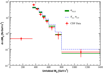
While both CDF and D0 have measurements of the invariant mass distribution Aaltonen:2009iz ; D0:winter2009 , only CDF presents an unfolded differential cross section. Therefore, we inspected the invariant mass spectra reported by CDF; see Fig. 1. We take the 7 bins with GeV in our fit and weight their by the number of included bins. This assigns an equal weight between the measurement and the and measurements.
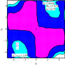
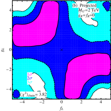
The observables are in addition to the binned data and define the output set. We use the combined cross section of Eq. (9). We therefore assign and in our implementation of the likelihood defined above for the case we denote as “Current” ( for , for , and for ) while and for the case we denote as “Projected,” where of integrated luminosity is used for each measurement, in which we assume the central values are fixed and the uncertainties are scaled by a factor . We combine the chains to form iso-contours of , , and significance via their respective -values.
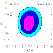
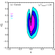
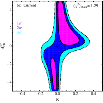
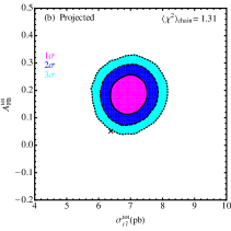
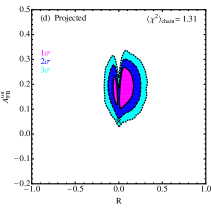
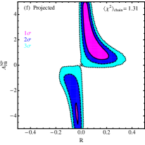
For illustration, we plot these contours in the plane of and in Figs. 2(a). We note that the current average values of and are consistent with the SM within the level. With an upgraded integrated luminosity of at the Tevatron, the statistical uncertainty would be reduced significantly; see Fig. 2(b). The deviation of from zero is then larger than . Note that we also allow negative values of in this work, though they are not preferred. Taking the SM theory prediction, we translate into defined in Eq. (6). The correlation of and is shown in Figs. 2(c) and (d). Finally, using Eq. (5), we obtain the correlation between and shown in Figs. 2(e) and (f). Clearly, the smaller the larger ; see the contour (solid black).
Note that since the MCMC is sensitive to the relative likelihood change in going between two points, it is sensitive to only the values. Therefore, the iso-contours of the -values for 1, 2, and assume the given model. To obtain an overall indication of how well the model in question fits the data, we quote , the per degree of freedom values averaged over the entire chain. In cases where we include the constraint, , otherwise . This quantity is an overall estimate of the model’s consistency with the data. Generally, values of are considered fairly good fits, while values much beyond that are not considered very good.
One might be tempted to search for the parameter set that yields the best fit to the given data. However, this is doing so without regard to the level of fine-tuning required to find such a point. Explicitly, this can be seen as a set of points in parameter space by which the value is minimized, ideally to zero. However, if a small deviation from these points provides a large increase in , this particular set of points that provide a good fit can be seen as more fine-tuned compared with another solution set without such a steep increase in . Therefore, the MCMC approach does take into account the parameter space available that affords a good fit, preferentially solutions with low fine-tuning.
To compare the MCMC results of Fig. 2 and subsequent Figures, we ran a MCMC with a pure SM explanation by explicitly setting and to zero and scanning over Eq. 13 with gaussian priors. We find that
| (15) |
where “Current Luminosity” refers to the measurement of with an integrated luminosity of 4.6 fb-1 and the measurement of with an integrated luminosity of 3.2 fb-1. For the projected integrated luminosity of 10 fb-1, we assume the central values of and remain unchanged from the values taken in Eqs. 2 and 9 while the uncertainties reduce by a scale factor . When we examine specific models that could give rise to a larger than the SM, we must also take into account the distribution measurement. To compare these models against the SM, we again run a MCMC with a pure SM explanation scanning over and as above while also scanning over our NLO prediction (seen in Fig. 1) with gaussian priors for the last seven bins of the CDF distribution. The bin nearest threshold accounts for the majority of the total cross section. Since we already include the total cross section in our fit, we do not include this bin in our fit of the distribution so that we do not weight the total cross section too heavily. If we include the measurement of the distribution and perform a MCMC scan over the SM, we find
| (16) |
Here, “Current Luminosity” refers to the above values of integrated luminosity for the and measurements and 2.7 fb-1 for the measurement of the distribution. For the projected luminosity of 10 fb-1, we again assume that the central values of all measurements remain the same while their errors scale as . We note that the values of in Eq. (16) are less than those in Eq. (15). This is because is a per degree of freedom. There are two degrees of freedom in Eq. (15) and three in Eq. (16) with the addition of the distribution. The good agreement of the distribution in the SM with data (seen in Fig. 1) causes the per degree of freedom to decrease when it is included in the fit. When comparing models, we can say that if the value for a given model is less than that for the SM with the appropriate data into account, the model will provide a better overall fit to the data than the SM.
The forward-backward asymmetry, defined in terms of a ratio of cross sections, is very sensitive to the renormalization and factorization scales, and respectively, at which the cross sections are evaluated. The uncertainties in the cross section associated with those scales can be considered as an estimate of the size of unknown higher order contributions. In this study, we set and vary it around the central value of , where is the mass of the top quark. Typically, a factor of 2 is used as a rule of thumb. Large scale dependence in the LO cross section can be significantly improved by including the higher order QCD and EW corrections. In this work we calculate the SM top pair production cross section with the NLO QCD corrections. Unfortunately, the QCD corrections to the induced top pair production are not available yet. Therefore, we calculate the NP contributions only at LO and rescale them by the -dependent SM K-factors. Due to the mismatch between the SM and NP cross sections, calculated in this way depends on the choice of scale.
| LO | NLO | |||||
| 6.82 | 5.01 | 3.79 | 5.70 | 5.56 | 5.04 | |
| 0.37 | 0.24 | 0.17 | 1.00 | 0.90 | 0.74 | |
| 0.00 | 0.00 | 0.00 | 0.01 | -0.03 | -0.05 | |
| 0.00 | 0.00 | 0.00 | 0.01 | -0.03 | -0.05 | |
| 7.19 | 5.26 | 3.96 | 6.72 | 6.39 | 5.69 | |
| 0.05 | 0.05 | 0.04 | 0.15 | 0.14 | 0.13 | |
| 0.93 | 1.22 | 1.42 | ||||
Table 1 shows the LO and NLO top quark pair production cross sections in the SM at the Tevatron. We present the quark annihilation and gluon fusion processes individually as well as their sum. The CTEQ6.6M Nadolsky:2008zw and CTEQ6L Pumplin:2002vw PDF packages are used in the NLO and LO calculations, respectively. In the last row we also list the K-factor, defined as the ratio of NLO and LO cross sections, for three scales.
We argue that the higher order corrections cannot be estimated by a K-factor (defined as the ratio of NLO and LO cross sections) because the K-factor is very sensitive to the scale. Furthermore, the gluon fusion channel contributes much more at the NLO (roughly about of total cross section) than at the LO (only about ). Hence, one also needs to take account of the gluon fusion channel contribution when calculating .
Another uncertainty originates from the top quark mass. In Table 2 we show the top pair production cross section for various top quark masses and three scales. The central values of NLO theory calculations for the three masses are always below the recent CDF results given in Eqs. (7) and (8), suggesting that the NP should contribute positively to production.
| LO | NLO | |||||
|---|---|---|---|---|---|---|
| 171.0 | 8.08 | 5.91 | 4.45 | 7.61 | 7.23 | 6.44 |
| 172.0 | 7.84 | 5.74 | 4.32 | 7.37 | 7.01 | 6.24 |
| 172.5 | 7.72 | 5.66 | 4.26 | 7.25 | 6.90 | 6.14 |
| 173.0 | 7.61 | 5.57 | 4.19 | 7.14 | 6.79 | 6.05 |
| 174.0 | 7.40 | 5.42 | 4.07 | 6.92 | 6.58 | 5.86 |
| 175.0 | 7.19 | 5.26 | 3.96 | 6.72 | 6.39 | 5.69 |
| 176.0 | 6.98 | 5.11 | 3.84 | 6.51 | 6.19 | 5.51 |
| 177.0 | 6.78 | 4.96 | 3.73 | 6.31 | 6.01 | 5.35 |
In the following sections, we study a few interesting new physics models which can generate a significant deviation from the SM expectation for in the top quark pair production channel. We also comment on the scale dependence in each new physics model. Without losing generality, in the rest of this paper, we set .
III Exotic gluon
We begin with an exotic gluon () model, as the other models can be easily derived from the model result. In Sec. III.1 we present analytic formulae for and . We calculate its width in Sec. III.2. In Secs. III.3, III.4, and III.5 we perform MCMC scans over parameters in several scenarios subject to the experimental constraints.
III.1 Differential cross section and asymmetry
The boson couples to the SM quarks also via the QCD strong interaction,
| (17) | |||||
| (18) |
where we normalize the interaction to the QCD coupling, , and use to denote light quarks of the first two generations. Such an exotic gluon can originate from an extra-dimensional model such as the Randall-Sundrum (RS) model Djouadi:2009nb , chiral color model Pati:1975ze ; Hall:1985wz ; Frampton:1987dn ; Frampton:1987ut ; Bagger:1987fz ; Cuypers:1990hb ; Cao:2005ba ; Carone:2008rx ; Ferrario:2008wm ; Martynov:2009en , or top composite model Contino:2006nn . As discussed below, the axial coupling of to the SM quarks is necessary to create a forward-backward asymmetry. In the extra-dimensional model, such non-vector coupling of Kaluza-Klein gluons to fermions arises from localizing the left- and right-handed fermions at different locations in the extra dimension.
The differential cross section with respect to the cosine of the top quark polar angle in the center-of-mass (c.m.) frame is
| (19) |
where
| (20) | |||||
| (21) | |||||
| (22) | |||||
Here the angle is defined as the angle between the direction of motion of the top quark and the direction of motion of the incoming quark (e.g., the -quark) in the c.m. system. The subscripts “SM”, “INT” and “NPS” denote the contribution from the SM, the interference between the SM and NP, and the NP amplitude squared. For the model, the SM contribution is from the gluon-mediated -channel diagram, the NPS contribution from the exotic gluon -mediated diagram, and the INT contribution from the interference between the two. The squared c.m. energy of the system is , and is the top quark velocity in the c.m. system.
The forward-backward asymmetry of the top quark in the c.m. frame is defined as
| (23) |
where
| (24) |
We further parameterize the differential cross section as follows:
| (25) |
where the subindex denotes “SM”, “INT” and “NPS”. Hence, after integrating over the angle , we obtain the asymmetry and total cross section
| (26) |
where the sums are over the SM, INT and NPS terms. In reality the incoming quark could originate from either a proton or an anti-proton, but it predominantly comes from a proton due to large valence quark parton distribution functions. Taking the quark from the anti-proton and the anti-quark from the proton contributes less than 1% of the total cross section. Therefore, in collisions at the Tevatron one can choose the direction of the proton to define the forward direction.
Now let us comment on a few interesting features of the asymmetry and cross section generated by the INT and NPS effects individually, because both effects are sensitive to different new physics scales: the former to a higher NP scale and the latter to a lower scale. First, we note that the asymmetry is sensitive to the ratio of coupling (squared) differences and sums for the INT (NPS) effects, e.g.,
| (27) | |||||
| (28) |
where and denote the averaged and after integration over the angle and convolution of the partonic cross section with parton distribution functions.
To make the physics source of the asymmetry more transparent, we define the reduced asymmetry () and reduced cross section as follows:
| (29) | |||||
| (30) | |||||
| (31) | |||||
| (32) |
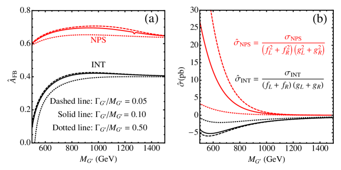
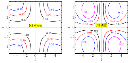
The reduced asymmetries and cross sections are easily computed universal functions that allow us to focus on two separate limiting cases; the new physics contribution to and is primarily from the INT term if it is produced by a heavy resonance that interferes with the SM production process. If the new physics is due to a resonance that doesn’t interfere with the SM production, then the new contribution to and is given by the NPS term. One simply has to multiply the reduced asymmetry or cross section by the appropriate combination of couplings to obtain the full new physics contribution to and . In Fig. 3 we plot the reduced asymmetry (a) and the reduced cross section (b) as functions of for various choice of . The reduced asymmetry generated by the INT effects increases rapidly with increasing and finally reaches its maximal value . The reduced asymmetry generated by the NPS effects is large, typically around 0.6-0.7. As expected, the reduced cross section of the NPS effects is alway positive; cf. the upper three curves in Fig. 3(b). On the other hand, the reduced cross section of the INT effects is always negative due to () in the numerator of Eq. (21). Both reduced cross sections, especially the NPS effects, are sensitive to the decay width. They both go to zero when decouples.

The difference between the two reduced asymmetries can be easily understood from the distribution shown in Fig. 4. Figure 4(a) shows the normalized differential cross section with respect to for 175 GeV top quark production in the SM at the Tevatron, which peaks around . The INT effects only slightly shift the peak position. Substituting into Eqs. (27) and (29), we obtain . On the contrary, the NPS effects prefer a much larger enforced by the heavy resonance. We plot in Fig. 4(b), where for a 2 TeV . Such a large leads to the large value of in Fig. 3. For an extremely heavy , is equal to 1, yielding the well-known maximal . When both INT and NPS effects contribute, one cannot factorize out the couplings as in Eqs. (27-32) due to the presence of both linear and quadratic coupling terms.
III.2 decay width
The term contributes significantly in the vicinity of where the decay width plays an important role. Hence, it is very important to use an accurate decay width in the parameter scan. We consider the case that the boson decays entirely into SM quark pairs, yielding the following partial decay width Ferrario:2008wm :
| (33) | |||
| (34) | |||
| (35) |
where denotes the light quark flavors and we have assumed that couples to with the same strength as . In the limit of , the total decay width of is
| (36) |
When the couplings are of order 1, . When , . In the following parameter scan we vary the couplings of the boson in the range of to when all couplings are present but to when only two are non-zero.
III.3 Left-handed :
Since there are five independent parameters (four couplings and the boson mass) in Eqs. (19-22), we turn off the right-handed couplings and in order to make the physics origin of the asymmetry more transparent. We first consider in Sec. III.3.1 and then in Sec. III.3.2. We will comment on non-zero and in Secs. III.4 and III.5.
III.3.1
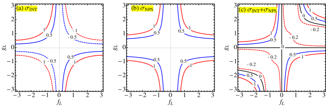
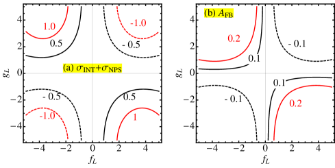
We first examine theoretical predictions of and and before we perform a MCMC scan over the parameters. By “theoretical” we mean that the asymmetry and the top pair production cross section are calculated independently, without regard to their correlation. Fig. 5(a) displays the cross section contours generated by the INT effects (). The INT effects could be either positive or negative, depending on the sign of the coupling product . The INT effects dominate in the region of , so their contribution to the top pair production cross section can be written as
| (37) |
This expression thus yields a positive contribution to the cross section when (i.e., the second and fourth quadrants in Fig. 5) and a negative contribution when (i.e., the first and third quadrants).
On the contrary, the NPS contribution is always positive; see Fig. 5(b). Since the NPS effects contribute mainly in the vicinity of , i.e. , their contribution to the top pair production cross section can be written as follows:
| (38) |
Hence, the contour pattern of is determined by . Fig. 5(c) shows the competition between the INT and NPS effects. For a , the INT generally dominates over the NPS. Note that the contours of net cross section are not symmetric between and due to the width effects. In Fig. 5(d), we see that, except for small couplings in the upper-right and lower-left quadrants, a positive asymmetry can be generated in all four quadrants. In the upper-right and lower-left quadrants, for , the NPS term is large enough to generate a positive . Note that negative values of , although not plotted in Fig. 5(d), are still consistent with the Tevatron data within C.L. and are included in the following analysis.
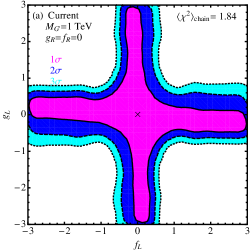
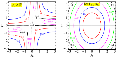
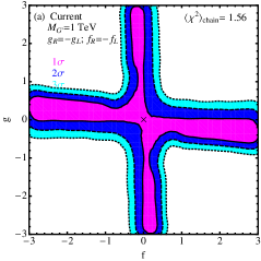
Now we perform a MCMC scan over the parameter space after combining measurements of the asymmetry, the total cross section, and . To obtain the distribution, we separate the contribution from the initial state (which includes the NP that we analyze) from that of the initial state, noting that the and contributions are negligible as seen in Table 1. We multiply these leading order results by the SM K-factors, and respectively, which are obtained by using the Monte Carlo program MCFM Campbell:2000bg to calculate the full NLO SM differential cross section. Each K-factor itself differs as a function of (as seen in Ahrens:2009uz ) and so we weight each bin in the distribution by the appropriate K-factors. We vary the scale at which we evaluate the NLO differntial cross section between and which gives a range of K-factors for each bin. This is used in our fits as our estimate of the theoretical uncertainty. This uncertainty is about 10% in the first six bins and around 15% in the last bin. Observe that this procedure, when NP effects are decoupled, reproduces the exact NLO SM differential cross section seen in Fig. 1. In this and subsequent Figures of MCMC distributions, we adopt flat priors in all variables scanned. The priors for the SM-only contribution to the cross section and are given in Eq. (13). Fig. 6(a) displays the parameter space consistent with both measurements at the (innermost region), (next-to-innermost region) and (outermost region) level, respectively, for . Remember, the iso-contours of the -values for 1, 2, and assume the given model, while the value gives an indication of the overall fit. In this case, we get a somewhat worse fit to both experimental results than in the SM, with . Fig. 6(b) shows the estimated parameter space contours with an integrated luminosity of , assuming the central values of both experimental measurements are not changed. The quality of the fit is marginally better than in the SM, with vs. 4.22 in the SM. We observe that the regions where or are small provide the best fit. The boundaries of all three contours can be understood from the theoretical predictions in Figs. 5(c) and (d). To explain the discrepancy in the total cross section and in the asymmetry, values of and in the top-left or bottom-right quadrants would be preferred. However, couplings here inevitably worsen the distribution. In the top-right and bottom-left quadrants the fit to the distribution is improved for small couplings () but the agreement with the total cross section is slightly worse and an asymmetry smaller than the SM value is generated. For intermediate couplings in these two quadrants (), the fit to the distribution is improved but the total cross section is reduced too much and the asymmetry is not improved significantly. Eventually, at large values of the couplings in these quadrants (), a large asymmetry is generated and the fit to the total cross section is improved but the distribution is greatly worsened. Furthermore, we note that the bands along the axis are slightly wider than those along the axis due to the asymmetric contributions of and to , cf. Fig. 5(e).
III.3.2
When the boson is very heavy, only the interference term in Eq. (21) contributes to , leading to
| (39) |
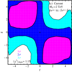
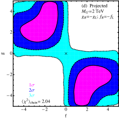
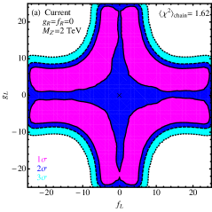
This dependence is illustrated in Fig. 7. In order to get positive corrections to and the top pair production cross section, the product needs to be negative to compensate the negative sign from the denominator of the propagator which is what we see in the upper left and lower right quadrants of Figs. 7 (a) and (b). The results of the MCMC scan are shown in Fig. 8 for . The contours look quite different from those in Fig. 6. We note that values of and in the upper-left and lower-right quadrants are preferred which is where a large positive asymmetry is generated as seen in Fig. 7. This shows that the distribution is less constraining than in the case as one would expect. The fit to the three experiments gives for the current integrated luminosity which is slightly better than in the SM where . The fit is improved relative to the SM at the upgraded luminosity with if the central values do not change as compared to the SM value of .
In Fig. 8, we observe that the upper-right and lower-left quadrants are not as tightly constrained as in the case in Fig. 6. Here, the distribution is improved.111Naively, one might expect that the distribution would not be very important for a with . However, for couplings the width of the can be comparable to (for , ) and the can contribute to the bin. In the case of the large couplings in these quadrants decrease the total cross section and asymmetry too much. However, in the case for large couplings in the upper-right and lower-left quadrants the NPS term becomes important due to the large width effects and this can mitigate the negative contribution to and from the INT term allowing for a better fit. This is why the and regions are not tightly constrained in the upper-right and lower-left quadrants for a in Fig. 8. Again, we note that the bands along the and axes are not symmetric due to their asymmetric contributions to .
III.4 Axi-gluon: and
Now we study the axi-gluon case, in which only has axial couplings to the quark sector. This type of model has been explicitly proposed as an explanation of the measurement without significantly affecting the total cross section Frampton:2009rk . There, the SM prediction for the cross section was taken to be larger than our value due to differences in and including incomplete NNLO calculations. Therefore, they did not need a significant correction to the cross section.

In the axial limit, only the asymmetry-generating term of the INT in Eq. (22) remains. In general, all terms in the NPS remain. Therefore, at large , the INT term dominates and a rather large asymmetry can arise without a sizable contribution to or to . At lower values of , the NPS term is increasingly relevant.
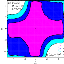
III.4.1
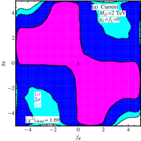
We show theoretical contours of (since vanishes when integrated over in the axi-gluon case) and in Fig. 9(a) and (b) for an axi-gluon of mass . We observe that a positive asymmetry is generated when the product , with and , is negative as we expect from Eq. 21. In Fig. 10(a) and (b), we perform MCMC scans and find a fit with for the current luminosity and for 10 fb-1 assuming the central values of the measurements do not change. Small values of either or are preferred due to the constraint on the distribution. These values of for the axi-gluon are better than the corresponding values in the SM fit. This indicates that a axi-gluon has less tension with the current data than the SM and would also offer an improvement over the SM if the central values of the data remain the same with an upgraded luminosity of .

III.4.2
For a axi-gluon, we plot theoretical contours of and in Fig. 9 (c) and (d). In Figs. 10(c) and (d), we show the results of a scan in the case of an axi-gluon with . The fit shows better agreement with the data in this case than in the SM, with for the current luminosity and for 10 fb-1 if the central values do not change. Due to the lessening of the constraint for a heavier axi-gluon, the scans show somewhat different structure than in the case. The allowed regions are located in the quadrants where which is where a positive is generated as seen in Fig. 9 (d). The regions of large coupling are constrained by the distribution. There is again a slight asymmetry in the width of the allowed regions near the and axes due to the asymmetry in the width.
Our results suggest that a heavy axi-gluon can offer a good explanation of the large observed without increasing the disagreement in the distribution too much, as proposed in Ref. Frampton:2009rk .
III.5 Other combinations of couplings

Now let us study different combinations of couplings, e.g., , and . Fig. 11 shows the MCMC scan results of various combinations of couplings with and with the current luminosity. Purely right-handed couplings in the -- interaction give rise to the exactly same result as purely left-handed couplings, cf. Fig. 8(a). But mixed combinations of left-handed and right-handed couplings, e.g., and , result in a worse fit, with , which is worse than the SM. This is mainly due to the INT effects which are sensitive to the signs of couplings; see Eqs. (21) and (27). Choosing or causes the INT effects to generate a negative , leading to the bad fit.
IV Effective field theory
For a boson, due to the broad decay width, the NPS contribution is still sizable for large couplings in the above MCMC scans. It is interesting to ask what the effects are if only the INT term contributes. To that end, in this section we consider dim-6 effective operators that can interfere with the SM top quark pair production channel . We further assume that the scale of the new physics is large enough that the NPS contributions (i.e. with the new physics scale) can be neglected. For illustration we focus only on the operators which couple left-(right-)handed light quarks to left-(right-)handed top quarks so that contact with Sec. III.3 can be made. They are listed as follows:
| (40) | |||||
| (41) | |||||
| (42) | |||||
| (43) |
where and denote the doublets of the light (first two generation) quarks and heavy (third generation) quark, respectively, and are the right-handed gauge singlets. Here, and are the and matrices; appropriate contractions are understood. The first index in the superscripts of operators labels the color octet and the second index denotes the weak isospin. Other color and weak singlet operators are omitted as they cannot interfere with the SM channel.
The effective Lagrangian of the four fermion interaction is thus given by
| (44) |
where we explicitly factor out a strong coupling strength , and the reduced coefficients are given as follows:
Here the generators are omitted and denotes the new physics scale.
The differential cross section of the EFT can be easily derived from Eq. (21) by taking the limit of ,
| (45) |
Obviously, the coefficients only affect but not . We extract the cutoff scale and coefficients as follows:
| (46) |
which yields, after integration over and convolution with PDFs,
The parameters () are listed in Table 3 for various choices of factorization scale, where and are evaluated using Eq. (26). It is clear that one needs positive or to get positive but this inevitably gives rise to a negative contribution to . Hence, it is difficult to fit both the asymmetry and the top pair production cross section simultaneously at the level.


| -0.294 | -0.256 | -0.092 | 0.395 | -0.648 | -0.052 | -0.040 | -0.040 | 0.355 | -0.113 | |
| -0.215 | -0.185 | -0.066 | 0.392 | -0.473 | -0.037 | -0.0288 | -0.10 | 0.353 | -0.062 | |
| -0.165 | -0.141 | -0.050 | 0.389 | -0.363 | -0.028 | -0.022 | -0.007 | 0.350 | -0.082 | |
Since one cannot separate the coefficient from the cutoff , we scan over the combination and limit ourselves to the region of in the MCMC scan. In Fig. 12 we plot the correlations between and (top row) and between and (bottom row). For the current luminosity, the fit quality of the EFT is worse than the SM, . The fit is marginally better than the SM, , for an integrated luminosity of 10 fb-1 if the central values of the measurements remain the same. The fit is worse than that of the left-handed due to the lack of a NPS term to balance the contributions of the INT term. This indicates the importance of resonance effects in the fit.
V Flavor-conserving boson
An additional can generate a nonzero if its coupling to quarks does not respect parity,
| (47) | |||||
| (48) |
where denotes the electromagnetic coupling strength. In contrast to , there is no interference between the -mediated top quark pair production and the SM process. Even though the amplitude interferes with the SM process , the latter contribution is negligible at the Tevatron. Only the NP resonance itself contributes to when the collider energy is large enough to see the resonance effects. We consider the case where both the up and down quarks are gauged, but it is also possible to gauge the up and down quarks differently Rosner:1996eb .
Since the interference is absent for the color singlet , only contributes to NPS. For the -channel diagram, the differential cross section of can be easily derived from that of by omitting the color factor in Eq. (22) and replacing by , yielding
| (49) | |||||
Negative searches for the boson at the Tevatron impose several lower bounds on the mass, roughly above 1 TeV for couplings of order electroweak size. For a leptophobic boson, the bound is slightly looser, . Owing to the rapid drop of the PDFs, the boson contributes significantly only in the resonance region, where . Further noting that the coefficient of the term in Eq. (49) is always less than one, we can drop this term and obtain
| (50) |


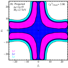
As in the study, we turn off the right-handed couplings first. Fig. 13 displays the correlation between and couplings for a 1000 GeV boson with . Like the 1 TeV , the distribution favors smaller or . The fit is worse than in the SM with for the current luminosity and for if the central values remain the same. For a 2 TeV boson with , we see the results of the MCMC scan in Fig. 14. The fit is somewhat better than the SM: for the current luminosity and for due to the lessening of the importance of for the higher mass . Furthermore, large couplings are allowed at the level. However, note that the unitarity constraint derived for the process requires ; see Appendix A for further details. Now, the heavy contributions are very sensitive to width effects. For we obtain . The positive contributions to the distribution, particularly in its last bin, are somewhat constrained. We conclude that this model can offer a small improvement over the SM in describing , , and the invariant mass distribution simultaneously.
VI Flavor-violating and models
In this section we consider a flavor-violating model, which includes a -- interaction. Such a FCNC could appear at tree-level or loop-level. Rather than focus on a specific model, we consider the following effective coupling of -- Jung:2009jz :
| (51) |
where denotes the electromagnetic coupling strength. In addition to the SM QCD production channel, , the top quark pair can also be produced via the process with a -channel boson propagator. The top quark asymmetry is naturally generated by this new process which also interferes with the SM production mode. Therefore, the differential cross section versus the cosine of the top production angle is given as follows Cheung:2009ch :
| (52) |
where
| (53) | |||||
| (54) | |||||
and is given in Eq. (20). The interference between the QCD and EW processes can be easily understood as follows. The gluon propagator can be split into a gluon propagator and a gluon propagator Maltoni:2002mq ,
| (55) |
where the gluon, carrying a factor , is unphysical. Color flow of the SM QCD channel (i.e., and ) is then exactly the same as the induced -channel diagram, resulting in interference between both processes.
Within the SM, the FCNC coupling -- vanishes at tree-level, but can be generated at one loop. However, the one-loop generated coupling is strongly suppressed by the GIM mechanism, making the FCNC top interactions very small. In models beyond the SM this GIM suppression can be relaxed, and one-loop diagrams mediated by new particles may also contribute, yielding effective couplings orders of magnitude larger than those of the SM. Since the coupling strength of this FCNC interaction is typically at the order of the SM weak interaction, the coefficients and are expected to be much smaller than 1. Therefore, it is not easy to generate a large asymmetry from a loop-induced -- interaction. However, the couplings and could be larger if they are generated at tree-level.
While the value of is not well constrained by direct or indirect search experiments, the value of is tightly bounded by the -sector. The left-handed coupling in Eq. (51) originates from the gauge interaction of the boson to the first and third generation quark doublets,
| (56) |
where denotes the first (third) generation quark doublet and the covariant derivative is , where is the charge. The flavor violating interaction -- then follows directly from the gauge invariance, which can contribute to the - mixing at the tree level 222 A similar correlation among the gauge boson and the third generation quarks in the SM has been studied in Ref. Berger:2009hi .. A coupling of the form
| (57) |
follows from Eq. 56 after rotating to the mass eigenstate basis with as in Eq. 51 and and elements of the CKM matrix. Assuming no additional NP effects arise, this gives a contribution to the mass difference between - of
| (58) |
where is the decay constant and is the “bag parameter” that characterizes the deviation from the vacuum saturation approximation. If we conservatively require that this contribution does not exceed the experimental value of Amsler:2008zzb , we can set a limit on of
| (59) |
where we use Gamiz:2009ku and Amsler:2008zzb . As a result, we choose hereafter. Furthermore, the unitarity constraint derived for the process requires only ; see Appendix A for further details.
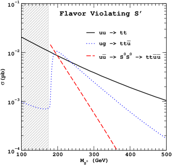
The most striking signal of the FCNC model is same-sign top pair production through the processes via a -channel diagram mediated by the boson. Recently, the CDF collaboration searched for the same-sign top pair signature induced by the maximally flavor-violating scalars at the Tevatron and found no evidence of new physics beyond the SM Aaltonen:2008hx . In their analysis, the upper limit to the production cross section of same-sign top pairs is of the order of . We show, in Fig. 15, the same-sign top production cross section at the Tevatron for couplings and . The cross section scales with the right coupling as if . Direct production via -channel exchange dominates and is severely constrained as the couplings increase. Note that we do not consider the possible effects that same-sign top production could have on a measurement of which requires a delicate analysis and will be presented elsewhere future .


In Fig. 16 we show the result of the MCMC scan in the plane of and : (a) for the current integrated luminosity and (b) for expected . For the current integrated luminosity, we impose the constraint of Aaltonen:2008hx , whereas for 10, we assume the cross section limit scales with , giving . The value of for the current integrated luminosity indicates that the FCNC model fits , and the distribution worse than the SM. Note the quality of fit is maintained even if we fix the mass to be specific values as in the flavor-conserving and cases. Since the INT effects lead to a negative asymmetry, one needs a large NPS contribution to overcome the negative INT contributions to generate the positive asymmetry. That requires a very large coupling, as seen in the upper and lower contours of Fig. 16(a) and (b), which is near the constraint of . In this model, the predicted value for the same-sign top pair production cross section is pushed to just below the limit taken. Overall, while there is tension between the positive asymmetry and small , we find a fit not much worse than the SM. With , the fit remains worse than in the SM with .
The observed top asymmetry may also be induced by a flavor-changing interaction via a charged boson Cheung:2009ch ; Barger:2010mw . The top quark pair can be produced in the channel via a -channel boson propagator. As in the flavor-violating case, we consider the following effective -- coupling:
| (60) |
where denotes the electromagnetic coupling strength. The differential cross section of is the same as Eq. (52) with the substitution .
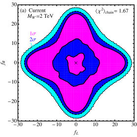
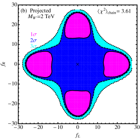
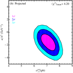
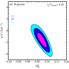
One advantage of the flavor-violating model is that it does not suffer from the constraint of same-sign top pair production at the Tevatron. Fig. 17 displays the correlation between and couplings for a 2000 GeV boson. For the current luminosity the contours are symmetric for and and the innermost one includes . In order to generate positive asymmetry, the couplings and need to be large enough to overcome the negative INT contributions. The typical values of couplings and are in the range of to . For the current luminosity, which indicates a better overall fit than the FCNC boson due to the lack of the same-sign top constraint, and a better fit than the SM. Due to the PDF dependence, the -quark initiated production via the is smaller than the -quark initiated production through a . Therefore, larger couplings are required to maintain the production cross section than in the case. With upgraded luminosity, provided that the central values of and are maintained which offers more improvement over the SM.
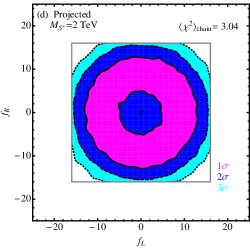
We focus on a heavy due to general constraints from electroweak precision and flavor measurements. In general, a is associated with a broken non-abelian gauge group and one must also consider a neutral gauge boson, , whose mass is typically degenerate or nearly so with that of the . If this has predominantly flavor-changing couplings to top quarks, then it falls into the previous case we analyzed. If its coupling to top quarks is flavor-conserving then one would expect to produce top quark pairs through s-channel exchange. However, such a process suffers from PDF suppression and is negligible in comparison to the contribution considered above and therefore we ignore it here. 333A model with a light and has been proposed in Ref. Barger:2010mw and may lead to a naturally good fit. This model has potential implications for precision electroweak observables which have not yet been fully explored.
VII Flavor-violating scalar
In addition to spin-1 exchange, we also consider the FCNC top interaction with a new color singlet scalar :
| (61) |
where is an doublet and we parameterize the overall coupling strength with respect to the weak coupling . If we assume to be the SM Higgs boson, then the FCNC top interaction originates from the dimension-6 operator
Results for this operator can be obtained from those for Eq. (61) with the substitution . As will be shown below, such an effective coupling is too small to generate a sizable asymmetry however. Hence, it is difficult to explain the asymmetry with the SM Higgs boson effective coupling without introducing additional heavy scalars.
The differential cross section is written as
| (62) |
where
| (63) | |||||
| (64) |
with . Due to the repulsive scalar interaction, the NPS contributions generate a negative . In order to generate a positive , the scalar needs to be very light, generally , and to have large couplings with the top quark. However, such a light scalar leads to a new top quark decay channel , which is tightly constrained Amsler:2008zzb . Therefore, we consider scalar masses that are larger than top quark mass to forbid this new decay channel. Furthermore, the flavor-violating coupling will be highly constrained by - mixing (a process) if one assumes a universal flavor-violating coupling among the three families of quarks. However, from a purely phenomenological perspective, we assume that the second generation quarks are not involved in the flavor-violating Yukawa interaction which leads to no constraint on the Yukawa couplings and . In other words, (,) is taken as a free parameter and is only constrained by considerations of unitarity (see Appendix A for details).


We plot as a function of for a scalar of mass in Fig. 18 (d) and see that it is indeed negative. This does not pose a problem with respect to the measurement of a positive asymmetry since the scalar interferes destructively with the SM which gives a negative , defined in Eq. (6) and shown in Fig. 18 (c). Thus, the total asymmetry, which is related to and in Eq. (5), is positive. This is plotted in Fig. 18 (a).
We also consider a charged scalar, , which couples to top quarks as in Eq. (61), but with the replacement . In Fig. 19, we see the result of the MCMC scan in the plane of and for a 1000 GeV neutral and charged scalar: (a,c) for the current luminosity and (b,d) for expected , again assuming the central value of experimental data is not changed. For the neutral scalar, we impose the same-sign top pair production constraint discussed in Sect. VI. We plot the same-sign top pair production cross section for a neutral scalar with at the Tevatron in Fig. 20. In the case of the neutral scalar, with the current luminosity we find a marginally better fit than in the SM, . The fit improves relative to the SM with for if the central values remain the same. For the charged scalar we obtain a similar fit at the current luminosity with . At with the same central values we obtain a slightly better fit, , than in the case of the neutral scalar due to differences between the and PDFs. Although the negative decreases the total cross section , it allows for good agreement with the distribution and gives a positive contribution to which results in a better overall fit.
VIII Conclusion
We have examined a number of models for new physics in top quark pair production which could account for the larger-than-expected forward-backward asymmetry observed at the Fermilab Tevatron, while not significantly disturbing the approximate agreement of the cross section and its distribution with the Standard Model predictions. Our results are summarized in Table 4.
| Model | Result | |
|---|---|---|
| FC | 1 TeV | Poor fit for considered due to constraint; |
| Good fit for axial couplings | ||
| 2 TeV | Fit not significantly improved with respect to the SM for ; | |
| Excellent fit for axial couplings | ||
| EFT | Poor fit; consistently smaller than measured value. | |
| FC | 1 TeV | Poor fit due to constraint |
| 2 TeV | Fit not significantly improved with respect to the SM for | |
| FV | Poor fit due to constraint and same-sign top constraint | |
| FV | 2 TeV | Good fit although large couplings necessary with a large amount of fine-tuning |
| FV , | 2 TeV | Tension with small predicted leads to poor fit with current data; |
| however, a good fit would be obtained if central values were unchanged after | ||
| Model | Total | ||||||
|---|---|---|---|---|---|---|---|
| FV : | 0.63 | 0.06 | 0.27 | 0.96 | 0.32 | 41.4% | 1.67 |
| axial : | 0.75 | 0.47 | 0.75 | 1.97 | 0.66 | 1.6% | 1.15 |
| chiral : | 0.59 | 2.91 | 0.62 | 4.12 | 1.37 | 0.4% | 1.69 |
| FC : | 0.67 | 2.66 | 0.91 | 4.24 | 1.41 | 1.0% | 1.62 |
| FV : | 2.01 | 2.85 | 0.09 | 4.96 | 1.65 | 0.2% | 1.72 |
| FV : | 2.01 | 2.85 | 0.12 | 4.98 | 1.66 | 0.2% | 1.72 |
| SM : | 1.12 | 4.07 | 0.06 | 5.25 | 1.75 | – | 1.75 |
The results summarized in Table 4 show that it is not easy to account for the larger-than-expected value of observed at the Fermilab Tevatron while maintaining the good agreement between theory and experiment for the production cross section and differential rate .
Of the models considered, those that provide a fit better than the SM for the applicable data are a or flavor-conserving with axial couplings, a (or a flavor-conserving or ) with chiral couplings. Other models we considered provide at most a mild improvement with respect to the SM case. The 1 TeV cases often give large corrections to the distribution since the additional signal is well inside the data region. Finally, in Table 5, we examine in detail the contribution to the in the small neighborhood around the best points in parameter space of the axial , chiral , FV chiral , and FC chiral models as well as the SM. Assuming the current integrated luminosity for each measurement and a mass of the new states responsible for the deviation of 2 TeV, we find:
-
•
The axial model provides the best overall fit to the experimental data considered in this article. It improves the agreement with experiment of both the total top quark production cross section and the forward-backward asymmetry. The fit to the distribution is slightly worse than in the SM case but still in good agreement with data.
-
•
The can also lead to a good fit to the data. It is able to generate a large asymmetry and to improve the agreement of total cross section with data without disturbing the differential cross section sizably for some regions of parameter space. However, large couplings are needed. Note that in Table 5, the best-fit point in the case has a lower than the axial although the is lower for the axial indicating that the axial gives a better overall fit. Stated differently, the requires a greater amount of fine-tuning of its parameters to fit the data than the axial . This is seen in the large value of ; a slight perturbation of the best fit points greatly decreases the quality of the fit. The model provides such a large value since the contributions from and are aligned and increase together with couplings that deviate from the minimum couplings. This is to be contrasted with the other models in which the increasing contribution from, say, is compensated by a smaller contribution from , resulting in a total value that remains relatively flat.
-
•
The chiral and do not lead to significant improvement over the SM. They reduce the discrepancy with the asymmetry measurement although they are unable to reduce it below without disturbing the distribution due to their large widths.
-
•
The FV scalars and have fits that are not significantly improved with respect to the SM. They lead to a significant discrepancy in and only slightly improve the fit to and with respect to the SM.
In this work, we have used the full NLO QCD production cross section. It is worth noting that partial NNLO QCD corrections to the cross section have been calculated in Ref. Kidonakis:2008mu and give rise to an enhancement of the total cross section of about 0.3 pb. This indicates that higher order QCD corrections might improve the agreement between the measured total cross section and its value in the SM, and therefore areas of NP parameter space which give negative contributions to the total cross section will be less constrained. Such negative contributions, however, may be in tension with the observed invariant mass distribution. A detailed collider simulation, including the complete NNLO corrections, would be therefore highly desirable in order to make a more reliable comparison of the predictions of these models with data.
Crucial to the test of any model is also the accumulation of more integrated luminosity at the Tevatron, in order to demonstrate deviations from the Standard Model exceeding . Until then, the observed values cannot be regarded as anything more than a hint of new physics.
Acknowledgements.
Q.-H. C. is supported in part by the Argonne National Laboratory and University of Chicago Joint Theory Institute (JTI) Grant 03921-07-137, and by the U.S. Department of Energy under Grants No. DE-AC02-06CH11357 and DE-FG02-90ER40560. D. M. and J. L. R. are supported by the U. S. Department of Energy under Grant No. DE-FG02-90ER40560. G. S. is supported in part by the U. S. Department of Energy under Grants No. DE-AC02-06CH11357 and DE-FG02-91ER40684. C. E. M. W. is supported in part by U. S. Department of Energy under Grants No. DE-AC02-06CH11357 and DE-FG02-90ER40560. J. L. R., G. S., and C. E. M. W. thank the Aspen Center for Physics for hospitality. The authors thank M. Neubert for useful discussions.Appendix A Unitarity constraints
In this appendix, we explore the unitarity constraints on new physics models considered in this work. The weak isospin amplitude ( being isospin index) can be decomposed with respect to orbital angular momentum according to
| (65) |
With the normalization , the unitarity constraint requires
| (66) |
where could be projected via:
| (67) |
First consider the flavor-conserving models, which involve the -channel diagram only. Note that the constraints of the model can be easily derived from flavor-conserving model. The helicity amplitudes for are represented by , where , respectively, indicates a left-handed and a right-handed top quark. Apart from the common factor
the non-vanishing helicity amplitudes from the diagram mediated by the boson are
| (68) | |||||
| (69) | |||||
| (70) | |||||
| (71) | |||||
| (72) | |||||
| (73) | |||||
| (74) | |||||
| (75) |
where . In the c.m. frame of the pair the 4-momenta of the particles are chosen to be
| (76) | |||||
| (77) | |||||
| (78) | |||||
| (79) |
In the high energy limit , only terms contribute. The partial-wave of amplitude is
| (80) |
yielding the following limit . Similarly, one can derive the following constraints
from the and processes.
Now consider the flavor-violating model. We consider the scattering , the calculation of which is identical to the flavor-conserving model. In the high energy limit , we obtain the following unitarity bound on from the helicity amplitude in Eq. 74,
| (81) |
Finally, we consider the scattering to derive the unitarity constraint for the flavor-violating model. The helicity amplitudes are represented by . In the high energy limit , the non-vanishing helicity amplitudes are
| (82) | |||||
| (83) | |||||
| (84) | |||||
| (85) |
where and are given in Eq. 61. The partial-wave of is
| (86) |
yielding the unitarity limit . Hence, , , and .
References
- (1) CDF, G. Strycker et al., (2009), Public-Note::CDF/ANAL/TOP/PUBLIC/9724.
- (2) CDF, T. Aaltonen et al., Phys. Rev. Lett. 101, 202001 (2008), arXiv:0806.2472.
- (3) O. Antunano, J. H. Kühn, and G. Rodrigo, Phys. Rev. D77, 014003 (2008), arXiv:0709.1652.
- (4) D0, V. M. Abazov et al., Phys. Rev. Lett. 100, 142002 (2008), arXiv:0712.0851.
- (5) J. H. Kühn and G. Rodrigo, Phys. Rev. Lett. 81, 49 (1998), arXiv:hep-ph/9802268.
- (6) J. H. Kühn and G. Rodrigo, Phys. Rev. D59, 054017 (1999), arXiv:hep-ph/9807420.
- (7) A. Djouadi, G. Moreau, F. Richard, and R. K. Singh, (2009), arXiv:0906.0604.
- (8) S. Jung, H. Murayama, A. Pierce, and J. D. Wells, Phys. Rev. D81, 015004 (2010), arXiv:0907.4112.
- (9) K. Cheung, W.-Y. Keung, and T.-C. Yuan, Phys. Lett. B682, 287 (2009), arXiv:0908.2589.
- (10) P. H. Frampton, J. Shu, and K. Wang, Phys. Lett. B683, 294 (2010), arXiv:0911.2955.
- (11) J. Shu, T. M. P. Tait, and K. Wang, (2009), arXiv:0911.3237.
- (12) A. Arhrib, R. Benbrik, and C.-H. Chen, (2009), arXiv:0911.4875.
- (13) P. Ferrario and G. Rodrigo, (2009), arXiv:0912.0687.
- (14) I. Dorsner, S. Fajfer, J. F. Kamenik, and N. Kosnik, (2009), arXiv:0912.0972.
- (15) D.-W. Jung, P. Ko, J. S. Lee, and S.-h. Nam, (2009), arXiv:0912.1105.
- (16) J. Cao, Z. Heng, L. Wu, and J. M. Yang, (2009), arXiv:0912.1447.
- (17) V. Barger, W.-Y. Keung, and C.-T. Yu, (2010), arXiv:1002.1048.
- (18) CDF public note, http://www-cdf.fnal.gov/physics/new/top/2009/xsection/TopXsNN/topXs_46f%b_public.html .
- (19) CDF public note, http://www-cdf.fnal.gov/physics/new/top/confNotes/cdf9913_ttbarxs4invfb%.ps .
- (20) P. M. Nadolsky et al., Phys. Rev. D78, 013004 (2008), arXiv:0802.0007.
- (21) U. Langenfeld, S. Moch, and P. Uwer, Phys. Rev. D80, 054009 (2009), arXiv:0906.5273.
- (22) V. Barger, W.-Y. Keung, and G. Shaughnessy, Phys. Rev. D78, 056007 (2008), arXiv:0806.1962.
- (23) N. Kidonakis and R. Vogt, Phys. Rev. D78, 074005 (2008), arXiv:0805.3844.
- (24) P. Nason, S. Dawson, and R. K. Ellis, Nucl. Phys. B303, 607 (1988).
- (25) W. Beenakker, H. Kuijf, W. L. van Neerven, and J. Smith, Phys. Rev. D40, 54 (1989).
- (26) M. Cacciari, S. Frixione, M. L. Mangano, P. Nason, and G. Ridolfi, JHEP 09, 127 (2008), arXiv:0804.2800.
- (27) S. Moch and P. Uwer, Nucl. Phys. Proc. Suppl. 183, 75 (2008), arXiv:0807.2794.
- (28) CDF, T. Aaltonen et al., Phys. Rev. Lett. 102, 222003 (2009), arXiv:0903.2850.
- (29) D0 public note, http://www-d0.fnal.gov/Run2Physics/WWW/results/prelim/TOP/T83/T83.pdf .
- (30) J. Pumplin et al., JHEP 07, 012 (2002), arXiv:hep-ph/0201195.
- (31) J. C. Pati and A. Salam, Phys. Lett. B58, 333 (1975).
- (32) L. J. Hall and A. E. Nelson, Phys. Lett. B153, 430 (1985).
- (33) P. H. Frampton and S. L. Glashow, Phys. Lett. B190, 157 (1987).
- (34) P. H. Frampton and S. L. Glashow, Phys. Rev. Lett. 58, 2168 (1987).
- (35) J. Bagger, C. Schmidt, and S. King, Phys. Rev. D37, 1188 (1988).
- (36) F. Cuypers, Z. Phys. C48, 639 (1990).
- (37) Q.-H. Cao, S.-L. Chen, E. Ma, and G. Rajasekaran, Phys. Rev. D73, 015009 (2006), arXiv:hep-ph/0511151.
- (38) C. D. Carone, J. Erlich, and M. Sher, Phys. Rev. D78, 015001 (2008), arXiv:0802.3702.
- (39) P. Ferrario and G. Rodrigo, Phys. Rev. D78, 094018 (2008), arXiv:0809.3354.
- (40) M. V. Martynov and A. D. Smirnov, (2009), arXiv:0906.4525.
- (41) R. Contino, T. Kramer, M. Son, and R. Sundrum, JHEP 05, 074 (2007), arXiv:hep-ph/0612180.
- (42) J. M. Campbell and R. K. Ellis, Phys. Rev. D62, 114012 (2000), arXiv:hep-ph/0006304.
- (43) V. Ahrens, A. Ferroglia, M. Neubert, B. D. Pecjak, and L. L. Yang, (2009), arXiv:0912.3375.
- (44) J. L. Rosner, Phys. Lett. B387, 113 (1996), arXiv:hep-ph/9607207.
- (45) F. Maltoni, K. Paul, T. Stelzer, and S. Willenbrock, Phys. Rev. D67, 014026 (2003), arXiv:hep-ph/0209271.
- (46) E. L. Berger, Q.-H. Cao, and I. Low, (2009), arXiv:0907.2191.
- (47) Particle Data Group, C. Amsler et al., Phys. Lett. B667, 1 (2008).
- (48) E. Gamiz, C. T. H. Davies, G. P. Lepage, J. Shigemitsu, and M. Wingate, Phys. Rev. D80, 014503 (2009), arXiv:0902.1815.
- (49) CDF, T. Aaltonen et al., Phys. Rev. Lett. 102, 041801 (2009), arXiv:0809.4903.
- (50) Q.-H. Cao, D. McKeen, J. L. Rosner, G. Shaughnessy, and C. E. M. Wagner, in preparation.