Dynamics of colloidal particles with capillary interactions

Abstract

We investigate the dynamics of colloids at a fluid interface driven by attractive capillary interactions. At submillimeter length scales, the capillary attraction is formally analogous to two-dimensional gravity. In particular it is a non-integrable interaction and it can be actually relevant for collective phenomena in spite of its weakness at the level of the pair potential. We introduce a mean–field model for the dynamical evolution of the particle number density at the interface. For generic values of the physical parameters the homogeneous distribution is found to be unstable against large–scale clustering driven by the capillary attraction. We also show that for the instability to be observable, the appropriate values for the relevant parameters (colloid radius, surface charge, external electric field, etc.) are experimentally well accessible. Our analysis contributes to current studies of the structure and dynamics of systems governed by long–ranged interactions and points towards their experimental realizations via colloidal suspensions.

I Introduction

In recent years the issue of structure formation by colloids at fluid interfaces has been the subject of intense experimental and theoretical research. If the colloidal particles are only partially wetted by the coexisting fluids, for not too high concentrations a two–dimensional (2D) colloid layer forms at the fluid–fluid interface because the detachment energy of a particle from such an interface is much larger than the thermal energy Pieranski (1980); Chateau and Pitois (2003). It turns out that these systems provide an excellent test-bed for fundamental issues (such as, e.g., 2D phase transitions Zahn et al. (1999)) as well as interesting perspectives for a variety of applications (such as, e.g., micropatterning and novel materials emerging from particle self–assembly Velikov and Velev (2006)).

The colloidal particles forming a 2D layer at fluid interfaces interact with each other in diverse ways. For the present purpose, these interactions can be classified into three groups (see, e.g., Ref. Oettel and Dietrich (2008)). (i) There is the ubiquitous van der Waals force, complemented by double–layer electrostatic interactions. These are described by the Derjaguin–Landau–Verwey–Overbeek (DLVO) model (see, e.g., Ref. Kleman and Lavrentovich (2003)) and are relevant only if the particles have a chance to come sufficiently close, leading to coagulation. (ii) One can find also a repulsive interaction of longer range. The presence of unscreened charges on the particle surface exposed to a nonpolar fluid phase generates an unscreened dipole–dipole repulsion Hurd (1985); Frydel et al. (2007); Domínguez et al. (2008). If both fluids are dielectric, the same kind of repulsion can be created by polarizing the particles with an external electric field Aubry and Singh (2008). If the particles are paramagnetic, a repulsion arises between magnetic moments induced by an external magnetic field Zahn et al. (1999). If one of the fluids is a nematic phase, director deformations induced by the anchoring boundary conditions at the particle surface can also lead to an effective repulsion Smalyukh et al. (2004); Oettel et al. (2009). This second group of interactions is usually promoted in experiments with the aim to stabilize the colloids against coagulation, in which case one can effectively neglect the DLVO–type force, as we shall do in the following. (iii) Finally, upon integrating out the interfacial degrees of freedom one obtains an effective, capillary interaction due to the colloid–induced deformation of the fluid interface (see, e.g., Refs. Kralchevsky and Nagayama (2000); Domínguez (2010)). There are several ways how the particles can deform the interface. A capillary attraction arises if a vertical force is exerted on the particles, e.g., due to buoyancy Nicolson (1949); Chan et al. (1981); Kralchevsky et al. (1992), an external electric field Aubry and Singh (2008), or the effect of a substrate if the lower fluid is a film of finite thickness (see, e.g., Ref. Kralchevsky and Nagayama (2000)). If the particles are non-spherical or the wetting properties of their surfaces are not homogeneous, the fluid interface is deformed anisotropically and the ensuing capillary force is attractive or repulsive depending on the relative orientation of the particles Lucassen (1992); Stamou et al. (2000); Brown et al. (2000); Fournier and Galatola (2002); van Nierop et al. (2005); Danov et al. (2005); Loudet et al. (2005); Lehle et al. (2008); Loudet and Pouligny (2009); Madivala et al. (2009).

The interest in capillary forces on the micrometer scale intensified recently when it was proposed Nikolaides et al. (2002) as an explanation for the puzzling attraction observed Onoda (1985); Ghezzi and Earnshaw (1997); Ruiz-García et al. (1997); Stamou et al. (2000); Quesada-Pérez et al. (2001); Tolnai et al. (2003); Gómez-Guzmán and Ruiz-García (2005); Chen et al. (2005, 2006) between micrometer–sized particles which were supposed to exhibit only the kind of repulsion discussed above as point (ii). However, various theoretical studies Foret and Würger (2004); Oettel et al. (2005a); Würger and Foret (2005); Oettel et al. (2005b); Domínguez et al. (2008) have shown that under the prevailing experimental conditions the capillary attraction between two spherical micrometer–sized particles is too weak to be able to explain the observed attraction. The reported effect might even turn out to be just an artifact of the experimental sample preparation Fernández-Toledano et al. (2004). Nevertheless, the capillary forces between charged particles still remains a topic of current research interest (see, e.g., Ref. Boneva et al. (2009) for a recent study considering deviations from sphericity).

These theoretical studies concern only the interaction between two isolated particles. The capillary interaction in the submillimeter range is formally analogous to unscreened 2D electrostatics (or 2D Newtonian gravity) Domínguez et al. (2008) and thus non-integrable in the sense of equilibrium statistical mechanics: the energy of configurations governed by this interaction is hyperextensive and the capillary attraction could be the relevant driving force for collective, genuine many–body phenomena in spite of its relative weakness at the two–body level. One of the goals of the present study is the investigation of this possibility for the kind of presently accessible experimental setups. Pergamenshchik (2009) has recently pointed out the possible relevance of this many–body effect as an explanation of the stability of the clusters observed in colloids at fluid interfaces. We shall show, however, that this claim is actually unfounded.

The second goal of this work is to introduce a theoretical framework which addresses the dynamical aspects of collective evolution under capillary attraction. The corresponding studies published in the literature so far report on the motion of either a single particle exposed to an externally created interfacial deformation or of few particles, usually two, following their own capillary attraction. Usually the equation of motion is solved in the overdamped approximation in order to relate the velocity with the capillary forces, thus providing a means of interpreting the experimentally recorded particle position as a function of time (see, e.g., Ref. Petkov et al. (1995) and, more recently, Refs. Loudet et al. (2005); Vassileva et al. (2005); Boneva et al. (2009)). In Ref. Singh and Joseph (2005) the full combined problem of particle motion and hydrodynamic flows in the fluid phases is addressed numerically with due account of the interfacial deformation. This approach is applied to clusters of two to four millimeter–sized particles. On that scale, the capillary attraction is screened and effectively very short ranged because it decays exponentially beyond the capillary length, which is typically of the order of millimeter.

Beyond this interest in the detailed motion of individual particles it seems that little attention has been paid to the overall evolution of a colloid monolayer driven by its own, self–consistently determined capillary force field. In this respect we are only aware of Ref. Vincze et al. (2001), where the clustering is studied experimentally as well as by means of molecular–dynamics simulations and interpreted within the framework of a certain effective kinetics of aggregation. In an attempt to be as realistic as possible, this latter theoretical approach takes into account many effects simultaneously (capillary forces, DLVO interactions, solvation forces, fluid streaming by temperature inhomogeneities). As a consequence in this analysis the specific signature of the capillary interaction on the dynamics is masked. Here we study the evolution of the coarse–grained particle–density field, with the diffusion at the interface being driven by the interparticle capillary attraction at scales below the capillary length. This is addressed within the mean–field approximation as being appropriate for a non–integrable interaction at that range of scales. The problem has a formal resemblance with the evolution of a self–gravitating 2D fluid, which allows us to predict a phenomenology akin to the process of cosmological structure formation.

The present study can also be viewed as a contribution to current investigations of the structure and dynamics of systems governed by long–ranged interactions, which can exhibit rather peculiar properties Campa et al. (2009); Bouchet et al. (2010). Our analysis points towards explicit experimental realizations of such systems via colloidal suspensions.

In Sec. II the mean–field model is introduced. After some qualitative considerations illustrating the overall picture, the model is formulated in terms of a set of coupled equations for the particle number density at the interface and the mean–field interfacial deformation. In Sec. III the time evolution predicted by this model is analyzed within two different approximations which facilitate an analytical solution of the problem. We first investigate the linear stability of a homogeneous particle distribution and find a clustering instability, which is the analogue of the so-called Jeans’ instability studied in the astrophysical literature. Then we compute the non-linear evolution of a radially symmetric perturbation in the limit of strong capillary attraction (the so-called cold–collapse approximation following the cosmological terminology). In Sec. IV we analyze available experimental setups and conclude that there is an accessible range of parameters for which one can expect that the predicted phenomenology is observable. In Sec. V we discuss pertinent experimental observations reported in the literature in the light of our results as well as the precise relationship between our study and the work by Pergamenshchik (2009). Sec. VI summarizes our conclusions.

II Mean–field approach

II.1 Qualitative considerations

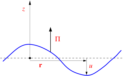
Figure 1: (color online) Small deformation (exaggerated in this schematic drawing) of a fluid interface (solid line). $u({\bf r})$ is the vertical deformation field (i.e., in $z$ direction) with respect to the reference, flat configuration (dashed line) as function of the lateral coordinate ${\bf r}=(x,y)$. $\Pi({\bf r})$ is the vertical force per unit area acting on the interface in the reference configuration. These two fields are related by Eq. (1).

We recall briefly the electrostatic analogy of small interfacial deformations, as worked out in Ref. Domínguez et al. (2008); Domínguez (2010) (see Fig. 1). Let $u({\bf r})$ denote the small vertical deformation of an otherwise planar interface at the lateral position ${\bf r}=(x,y)$, and $\Pi({\bf r})$ the vertical force per unit area exerted by external agents, e.g., a pressure imbalance across the interface or forces directly exerted on trapped particles (due to, e.g., buoyancy or optical tweezers). These two quantities are related by a Debye–Hückel–type equation,

$$\nabla^{2}u-\frac{u}{\lambda^{2}}=-\frac{1}{\gamma}\Pi,$$ (1)

where $\gamma$ is the surface tension and $\lambda$ is the capillary length. This equation describes local mechanical equilibrium: at each point of the interface, the force by external agents ($\Pi$) is counterbalanced by the surface tension of the curved interface ($\nabla^{2}u$), augmented by the force due to the weight of the fluid displaced relative to the flat configuration ($u/\lambda^{2}$). The lateral force on a piece $S$ of the interface exerted at its border by the rest of the interface takes the simple form

$${\bf F}_{\rm lat}=\int_{S}d^{2}{\bf r}\;\Pi({\bf r})\nabla u({\bf r}).$$ (2)

Equations (1) and (2) lead to the analogy that the deformation $u$ plays the role of a 2D electrostatic potential, $\Pi$ is the charge density, and the capillary length $\lambda$ is the screening or Debye length, with the peculiarity that the forces are reversed and charges of equal (different) sign attract (repel) each other. Or, in other terms, the analogy holds with a “screened” gravitational interaction involving positive and “negative” masses.

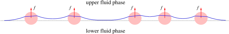
Figure 2: (color online) Side view of a fluid interface containing many particles, each subjected to a vertical external force $f$. Within the simplest approximation the particles are modelled as pointlike capillary monopoles of strength $f$.

In this respect, a particle trapped at the interface is characterized by a set of (capillary) multipolar charges and the lateral force is expressed in terms of the coupling of these multipoles with the deformation field $u({\bf r})$. Thus, similarly, the capillary interaction between a collection of particles (see Fig. 2) can be written as the sum of the interaction between pairs of multipoles localized at the position of the particles. In particular, the (isotropic) capillary monopole is simply equal to the net vertical force $f$ exerted on the particle by external agents, i.e., aside from the force provided by the interface Domínguez et al. (2008, 2005). The effective interaction between two monopoles of equal strength $f$ separated by a lateral distance $d\lesssim\lambda$ is described by the attractive potential Nicolson (1949); Chan et al. (1981); Kralchevsky et al. (1992); Domínguez (2010)

$$V(d)\approx-\frac{f^{2}}{2\pi\gamma}\ln\frac{\lambda}{d}\qquad(d<\lambda).$$ (3)

(Actually, the exact potential is given by $V(d)=-f^{2}K_{0}(d/\lambda)/(2\pi\gamma)$ in terms of a modified Bessel function; accordingly the length scale in the logarithm in Eq. (3) is $\approx 1.12\lambda$ instead of $\lambda$, but we neglect this small difference for the qualitative estimates to follow. At separations $d\gtrsim\lambda$, the interaction is screened and the potential crosses over to an exponential decay, which, for reasons of simplicity, we set to zero in the following reasoning.) This a 2D Coulombic interaction, which is known to be non-integrable and to drive an instability, e.g., in the astrophysically relevant case of a self–gravitating gas.

At this point we consider it to be useful to introduce a qualitative discussion which illuminates the physical origin of this instability. The more formally interested reader can skip this part without loss in favor of the mathematical derivation presented in the following sections. Consider a collection of $N\gg 1$ identical monopoles at positions ${\bf r}_{i}$ ($i=1,\dots,N$) distributed homogeneously over a region of linear extension $L$ (and thus of average number density $\varrho=N/L^{2}$). Due to the long–ranged nature of the interaction, the capillary energy per particle $e_{\mathrm{cap}}$ of the configuration can be estimated at the mean–field level as follows:

$$e_{\mathrm{cap}}=\frac{1}{2N}\sum_{i\neq j}V(|{\bf r}_{i}-{\bf r}_{j}|)\simeq\left\{\begin{array}[c]{lc}\displaystyle\frac{1}{2}\int_{r<L}d^{2}{\bf r}\;\varrho\,V(r)\sim-\frac{\varrho L^{2}f^{2}}{8\gamma}\left[1+2\ln\frac{\lambda}{L}\right],&\quad L<\lambda,\\ &\\ \displaystyle\frac{1}{2}\int_{r<\lambda}d^{2}{\bf r}\;\varrho\,V(r)\sim-\frac{\varrho\lambda^{2}f^{2}}{8\gamma},&\quad\lambda<L.\end{array}\right.$$ (4)

The key point is that for $L<\lambda$ this energy is not an intensive quantity but scales instead like $N=\varrho L^{2}$. There is also a contribution $e_{\rm short}$ to the energy per particle, due to thermal motion and short–ranged, predominately repulsive forces, which is $N$–independent. Therefore, if the system is large enough (but still $L<\lambda$) it can happen that the absolute value of the energy due to capillary effects $e_{\mathrm{cap}}$ ($<0$) dominates over $e_{\mathrm{short}}$ ($>0$). The corresponding critical system size can be characterized by Jeans’ length $L_{J}$ (this terminology is borrowed from the astrophysical literature), which is determined roughly by the condition $e_{\mathrm{short}}\simeq|e_{\mathrm{cap}}|$:

$$L_{J}\simeq\frac{1}{f}\sqrt{\frac{8\gamma e_{\rm short}}{\varrho}},$$ (5)

upon neglecting the logarithmic correction in Eq. (4). (A precise definition will be given in Sec. III, see, c.f., Eq. (19).) The capillary energy (Eq. (4)) can be expressed in terms of this length as follows:

$$e_{\mathrm{cap}}\simeq-e_{\mathrm{short}}\left(\frac{\lambda}{L_{J}}\right)^{2}\times\left\{\begin{array}[c]{cc}\displaystyle\left(\frac{L}{\lambda}\right)^{2}\left[1+2\ln\frac{L}{\lambda}\right],&L<\lambda,\\ &\\ 1,&\lambda<L.\end{array}\right.$$ (6)

One can distinguish two distinct extremal cases (see Fig. 3):

• $\lambda<L_{J}$: One can easily see that in this case $|e_{\mathrm{cap}}|<e_{\mathrm{short}}$, independently of the lateral extension $L$ of the homogeneous particle distribution and the effect of the capillary attraction is just a small perturbation. This case corresponds to the physical situation in which the capillary force is screened (i.e., negligible at distances beyond the capillary length $\lambda$) preempting that its cumulative effect becomes comparable with the net effect of the short–range forces associated with $e_{\mathrm{short}}$.

• $L_{J}<\lambda$: Here, $|e_{\mathrm{cap}}|>e_{\mathrm{short}}$ whenever $L_{J}<L$, implying that the homogeneous distribution is unstable because the attractive capillary force cannot be counterbalanced by the nonzero compressibility provided by $e_{\mathrm{short}}$. The system collapses into an inhomogeneous, clustered state with a new typical size $L^{*}$ and a new average density $\varrho^{*}$ sustained by its own capillary attraction energy $e_{\mathrm{cap}}^{*}$, and for which the compressibility provided by $e_{\mathrm{short}}^{*}$ can balance the capillary attraction so that $|e_{\mathrm{cap}}^{*}|\simeq e_{\mathrm{short}}^{*}$ (and the new, effective Jeans’ length $L_{J}^{*}$ is given by Eq. (5)). If Eq. (6) is evaluated for the quantities carrying an asterisk (characterizing the clustered state), this condition has two possible solutions:

  • the cluster size is of the order of its effective Jeans’ length, and the latter in turn is smaller than the capillary length, i.e., $L^{*}\sim L_{J}^{*}<\lambda$,

  • the effective Jeans’ length is of the order of the capillary length, and the latter in turn is smaller than the cluster size, i.e., $L_{J}^{*}\sim\lambda<L^{*}$.

  (In Appendix C we present an alternative qualitative derivation of condition (i) based on a force–balance argument rather than this energy consideration.)

These qualitative considerations are formalized in the following sections using a mean–field model for the particle dynamics under the action of capillary attraction.

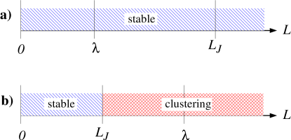
Figure 3: (color online) Qualitative stability diagram of the homogeneous distribution in terms of the capillary length $\lambda$ and Jeans’ length $L_{J}$ as a function of the system size $L$ for the two cases $\lambda<L_{J}$ (a) and $L_{J}<\lambda$ (b).

II.2 Mean–field capillary force

We consider a system of particles trapped at a fluid interface considered to be flat for the time being. In the absence of long–ranged interactions, there are equilibrium states corresponding to a 2D homogeneous fluid phase with areal particle number density $\varrho$, characterized by an equation of state $p(\varrho)$, where the “pressure” $p$ is the lateral force per unit length exerted by the particles on the walls providing the lateral confinement of the monolayer. (In what follows, we omit the possible dependence on the temperature $T$ which is irrelevant in the present context because we assume isothermal conditions maintained by the fluids on both sides of the interface.) One can write (setting the Boltzmann constant equal to unity)

$$p(\varrho)=\varrho T+p_{\rm ex}(\varrho),$$ (7)

where the first term is the entropic (ideal gas) contribution and the second term (excess pressure) is determined by the short–ranged interactions between the particles. There are always the hard–sphere contribution and the van der Waals attraction which eventually leads to colloid coagulation. However, in the experiments aimed at observing capillary effects these contributions are irrelevant because a longer–ranged repulsion (of electric, magnetic, or elastic origin) is implemented precisely to avoid coagulation Oettel and Dietrich (2008). Typically this repulsive potential has the simple form

$$v_{\rm rep}(d)=\frac{A}{d^{n}}=T\left(\frac{\zeta}{d}\right)^{n},\qquad(n>2),$$ (8)

where the constant potential parameter $A$ can be replaced by the Bjerrum length $\zeta=(A/T)^{1/n}$ of the potential (i.e., $v_{\mathrm{rep}}(d=\zeta)=T$, so that $\zeta$ decreases with increasing $T$). The repulsion of electric or magnetic origin corresponds to $n=3$ Oettel and Dietrich (2008); Domínguez et al. (2008), while the value of $\zeta$ can be varied via the externally controllable parameters of the system (strength of the external magnetic or electric field, water salinity, temperature, etc.). Because of the simple scaling behavior of this potential, the phase diagrams of such kind of fluids are determined by the single dimensionless parameter $\zeta^{2}\varrho$ (see, e.g., Ref. Hoover et al. (1971)): for sufficiently small $\zeta^{2}\varrho$ (high temperature, i.e., small $\zeta$, or low density) there is a fluid phase; if $\zeta^{2}\varrho$ is above a certain value, depending on $n$, the system freezes (for $n=3$ this threshold value is $\zeta^{2}\varrho\approx 4.6$ as obtained from experimental data Zahn et al. (1999)). Since the system is two–dimensional, the fluid–solid transition is expected to be of the Kosterlitz–Thouless type. For $n=3$ this is supported experimentally Zahn et al. (1999) and by recent simulations Lin et al. (2006), according to which there is a narrow range of values of the parameter $\zeta^{2}\varrho$ within which a hexatic phase is observed between the fluid and the solid phase.

In order to address the effect of the long–ranged capillary force, one introduces the ensemble–averaged interfacial deformation $U({\bf r})$. From Eq. (1) one obtains

$$\nabla^{2}U-\frac{U}{\lambda^{2}}=-\frac{f}{\gamma}\varrho,$$ (9)

in terms of the particle number density field $\varrho({\bf r})$. Here, the ensemble–averaged vertical pressure $\Pi({\bf r})$ has been replaced by the density of capillary monopoles,

$$\Pi({\bf r})=\Pi_{\rm mon}({\bf r})=f\varrho({\bf r}),$$ (10)

where the capillary monopole $f$ associated with a single particle is the net vertical force exerted on it by external agents. By analogy with 2D electrostatics and gravity, one can apply a mean–field approximation: the lateral capillary force experienced by a single particle located at ${\bf r}$ is written as $+f\nabla U({\bf r})$, after replacing the ensemble–average of $\Pi\nabla u$ in Eq. (2) by $f\varrho\nabla U$. Within this approximation correlations are neglected because $U({\bf r})$ is computed from the field $\varrho({\bf r})$ via Eq. (9), rather than from the density field conditional to the presence of a particle at ${\bf r}$. Therefore $U({\bf r})$ is actually the coarse-grained correlate of the interfacial deformation $u({\bf r})$, neglecting small–scale spatial variations. The physical assumption underlying the mean–field approximation is that the dynamics of a particle is predominantly determined by the simultaneous interaction with many other particles. This is usually expressed in terms of the constraint that the parameter $\varrho\lambda^{2}$ ($\sim$ number of neighbors which de facto exert a force on a particle) must be large. In the experiments of interest here this is always the case, because $\lambda\sim 1$ mm but the mean interparticle separation ($\sim\varrho^{-1/2}$) lies in the micrometer range. (Another implicit assumption, peculiar to the capillary problem, is that the capillary monopole $f$ of a particle is independent of the presence of other particles, i.e., of the particle density $\varrho$. This is a good approximation if the vertical force $f$ is predominantly due to gravity or due to an external electric or magnetic field, see, e.g., Ref. Oettel and Dietrich (2008) and references therein.)

In summary, the equilibrium state of the system is described macroscopically by the force balance equation

$$-\nabla p(\varrho)+f\varrho\nabla U={\bf 0},$$ (11)

which, together with Eq. (7) and Eq. (9), determines the equilibrium density profile $\varrho({\bf r})$. (Note that Eq. (11) also follows from, c.f., Eq. (14), or more generally Eq. (46), for $\partial\varrho/\partial t=0$.) Except for the finite value of the parameter $\lambda$ in Eq. (9), this problem is formally analogous to the Vlasov–Poisson model (corresponding to $\lambda=\infty$) for determining equilibrium configurations of a fluid under its own self–gravity Binney and Tremaine (2008) (see Ref. Sire and Chavanis (2002) for a comprehensive analysis of the equilibrium solution of the Vlasov–Poisson model for arbitrary spatial dimensions with $p_{\mathrm{ex}}(\varrho)\equiv 0$, i.e., for an ideal gas, see Eq. (7)). In recent years this old problem has received renewed attention and generalizations of it have been studied throughly (see Ref. Sire and Chavanis (2010) and references therein for a brief summary).

II.3 Diffusive dynamics

If the force balance equation (11) is violated, the particle density $\varrho({\bf r},t)$ will evolve in time according to the law of mass conservation, expressed by the continuity equation

$$\frac{\partial\varrho}{\partial t}=-\nabla\cdot(\varrho{\bf v}).$$ (12)

The flow velocity field ${\bf v}({\bf r},t)$ is determined by the law of motion of the particles. Each particle is dragged at the fluid interface by a mean force $-(\nabla p)/\varrho+f\nabla U$. We assume that the characteristic time scale of macroscopic evolution is long enough so that the motion of the particles at the interface occurs within the overdamped regime. This allows one to neglect particle inertia and a flow velocity is induced given by

$${\bf v}=\Gamma\left(-\frac{\nabla p}{\varrho}+f\nabla U\right),$$ (13)

where $\Gamma$ is a mobility coefficient of the particles at the interface. In addition there are hydrodynamic interactions between the particles due to the fluid flow induced by the particle motion which can affect the dynamical evolution Zahn et al. (1997). The effect of this interaction could be incorporated through a density dependence of $\Gamma$ (see, e.g., Ref. Batchelor (1972) for sedimenting hard spheres in bulk fluids) or, in a more explicit manner, by additional terms in the diffusion equation (14) below Rex and Löwen (2009). For our purposes, however, we neglect this effect and consider $\Gamma$ as a phenomenological input parameter which is taken to be spatially constant for reasons of simplicity. Inserting this flow field into Eq. (12) one obtains

$$\frac{\partial\varrho}{\partial t}=\Gamma\nabla\cdot[\nabla p(\varrho)-f\varrho\nabla U].$$ (14)

On the other hand, we assume that the evolution of the areal number density profile $\varrho({\bf r},t)$ occurs on a time scale sufficiently large so that deviations from local equilibrium and the presence of capillary waves can be neglected. Therefore, the equilibrium relationships in Eqs. (7) and (9) hold and, when combined with Eq. (14), a closed equation is obtained to determine the shape and the evolution of the density distribution $\varrho({\bf r},t)$, which thus follows a diffusive dynamics driven by “self–gravity”. As discussed in Appendix A the problem can be cast in terms of a functional formulation.

III Clustering instability

III.1 Linear stability of a homogeneous state

The occurrence of a clustering instability can be inferred from Eq. (14). For a macroscopically extended interface a homogeneous particle distribution of density $\varrho_{h}$ is a solution of Eqs. (9) and (11) with $U_{h}=f\lambda^{2}\varrho_{h}/\gamma$ ( = const.). We consider now a perturbed configuration $\varrho({\bf r},t)=\varrho_{h}+\delta\varrho({\bf r},t)$, $U({\bf r},t)=U_{h}+\delta U({\bf r},t)$ and linearize Eqs. (9) and (14) in terms of the small perturbations $\delta\varrho$ and $\delta U$:

$$\frac{\partial(\delta\varrho)}{\partial t}=\Gamma\nabla\cdot\left[\frac{1}{\varrho_{h}\kappa_{h}}\nabla\delta\varrho-f\varrho_{h}\nabla\delta U\right],$$ (15)

$$\nabla^{2}\delta U-\frac{\delta U}{\lambda^{2}}=-\frac{f}{\gamma}\delta\varrho,$$ (16)

where the isothermal compressibility $\kappa_{h}$ is given by

$$\kappa_{h}:=\left(\varrho\frac{\partial p}{\partial\varrho}\right)^{-1}_{T}(\varrho=\varrho_{h}).$$ (17)

We introduce the spatial Fourier decomposition of the perturbation,

$$\widehat{\delta\varrho}({\bf k},t)=\int d^{2}{\bf r}\;{\rm e}^{i{\bf k}\cdot{\bf r}}\delta\varrho({\bf r},t),$$ (18)

and define a characteristic wavenumber $K$ and a characteristic time ${{\cal T}}$ associated with the unperturbed homogeneous distribution as

$$K^{2}:=\frac{f^{2}\varrho_{h}^{2}\kappa_{h}}{\gamma},\qquad{{\cal T}}:=\frac{\gamma}{\Gamma f^{2}\varrho_{h}}.$$ (19)

The diffusion equation reduces to

$$\frac{\partial\widehat{\delta\varrho}}{\partial t}=\frac{1}{\tau(k)}\widehat{\delta\varrho}\qquad\Rightarrow\qquad\widehat{\delta\varrho}({\bf k},t)=\widehat{\delta\varrho}({\bf k},0)\,{\rm e}^{t/\tau(k)},$$ (20)

with a typical time of evolution $\tau(k)$ given by

$$\frac{1}{\tau(k)}=-\frac{\Gamma k^{2}}{\varrho_{h}\kappa_{h}}+\frac{\Gamma f^{2}\varrho_{h}}{\gamma}\frac{(\lambda k)^{2}}{1+(\lambda k)^{2}}=\frac{1}{{{\cal T}}}\left(\frac{k}{K}\right)^{2}\left[\frac{1}{(k/K)^{2}+(\lambda K)^{-2}}-1\right].$$ (21)

In the astrophysical literature (in which $\lambda=\infty$ for gravity, see, e.g., Refs. Binney and Tremaine (2008); Padmanabhan (2002) and references therein), $K$ is known as Jeans’ wavenumber (and $L_{J}:=1/K$ is the associated Jeans’ length, see Eq. (5)). The value of this parameter is determined by the properties of the unperturbed homogeneous state. Two qualitatively different cases can be distinguished (see Fig. 4):

• $\lambda K<1$, so that $\tau(k)<0$ for all values of $k$. In this case perturbations of all wavelengths decay exponentially as function of time; therefore the homogeneous state is stable. Physically, this describes the situation in which the number of particles inside the circle of interaction of radius $\lambda$ is too small and thus the capillary attraction is too weak to lead to a collapse of the colloidal fluid against a finite compressibility.

• $\lambda K>1$, so that $\tau(k)>0$ for wavenumbers below a critical one,

  $$k_{c}=K\sqrt{1-\frac{1}{(\lambda K)^{2}}},$$ (22)

  determined by the condition $\tau(k_{c})=0$. Perturbations satisfying this condition are linearly unstable, which describes the onset of a clustering instability. In the limit of no screening of the capillary attraction (i.e., for $\lambda\to\infty$), one recovers the scenario of Jeans’ instability: any homogeneous state is unstable against perturbations with a wavenumber smaller than Jeans’ wavenumber. Figure 5 depicts $k_{c}$ as function of $\lambda$: for all practical purposes one can take $k_{c}\approx K$ unless the parameter $\lambda K$ is close to one. As can be inferred from Fig. 4, ${{\cal T}}$ is the characteristic time of the fastest growing mode if $\lambda K$ is not too close to one.

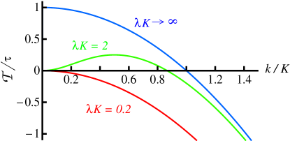
Figure 4: (color online) Inverse relaxation time $1/\tau(k)$ (Eq. (21)) as function of the wavenumber of the perturbation for different values of the parameter $\lambda K$. The units ${{\cal T}}$ and $K$ are given by Eq. (19). For $\lambda K<1$ one has $\tau(k)<0$ and thus linear stability against perturbations of all wavenumbers. For $\lambda K>1$ perturbations with long wavelengths are linearly unstable due to $\tau(k)>0$.

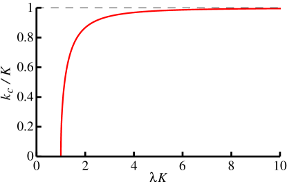
Figure 5: (color online) Dependence of the critical wavenumber $k_{c}$ (Eq. (22)) on the capillary length $\lambda$.

The value of Jeans’ length $L_{J}=1/K$ associated with every homogeneous configuration determines its stability against clustering by capillary attraction. If $L$ denotes the linear extension of the system, the results are summarized by Fig. 3 obtained previously in Subsec. II.1 based on qualitative arguments. The dependence of stability on the equation of state of each particular system enters only through the definition of Jeans’ length (Eq. (19)). A clustered phase is only possible if Jeans’ length is small enough, $\lambda K>1$, and the system size is sufficiently large, i.e., $2\pi<LK$, because a system of linear extension $L$ cannot support perturbations with wavenumbers smaller than $2\pi/L$. (Actually, if the system has a finite extension, the theoretical analysis above has to be complemented with appropriate outer boundary conditions compatible with a homogeneous particle distribution. We do not expect this to change the conclusions qualitatively, but maybe the precise value of $\lambda K$ setting the boundary of the stable region in Fig. 3.)

Finally, we remark that this Jeans–like instability has also been analyzed in two recent studies. In Ref. Sire and Chavanis (2008) a model of bacterial chemotaxis is considered, to which our equations reduce formally in a certain limit. In Ref. Chavanis and Delfini (2010) the same mathematical model as ours is studied except that the system is confined to a disk-shaped region with Neumann boundary conditions.

III.2 Cold collapse of a radially symmetric perturbation

Going beyond this simple linear analysis is possible only by resorting to numerical computations. There is, however, a case which can be addressed analytically: the dynamical evolution of a radially symmetric perturbation of a homogeneous background in the limit of vanishing Jeans’ length, meaning physically an arbitrarily compressible fluid (see Eq. (19)). In the cosmological literature this scenario is termed a “cold collapse” because in this context one considers ideal gases; for them an infinite compressibility amounts to a vanishing pressure $p(\varrho)$, which corresponds to the limit of zero temperature. The cold collapse is therefore the limiting case of a more general scenario involving both the capillary (gravitational) attraction and the pressure opposing compression. This approximation allows one to obtain an exact analytical solution of Eqs. (9) and (14) in the presence of radial symmetry in the limit $\lambda\to\infty$. The computational details are presented in Appendix C. Here we just summarize the results: The evolution of a localized radially symmetric perturbation of a homogeneous configuration is driven predominantly by the capillary attraction provided the system size is larger than Jeans’ length; in this case collapse occurs only if the spatially averaged density of the perturbation is larger than the one of the homogeneous start configuration (i.e., if there is an overdensity). The collapse proceeds until a cluster size of the order of the cluster Jeans’ length (i.e., the one associated with the density of the cluster) is reached and the pressure is able to halt the collapse. This last stage of the evolution, which does involve the effect of a finite compressibility, is beyond the cold–collapse approximation by construction and we have not studied it yet. The total time of collapse is given by Eq. (64) within the cold–collapse approximation and is roughly of the order of the characteristic time ${{\cal T}}$ associated with the homogeneous configuration (see Eq. (19)).

This exact solution of a simplified model can be used to gain some insight into a more realistic situation. Suppose that in a homogeneous configuration of density $\varrho_{h}$ Jeans’ length is small enough so that there can be found patches of linear extension $L<\lambda$ fulfilling the condition of instability, $L_{J}<L$ (see Fig. 3). In such a patch there are always thermally induced density fluctuations $\delta\varrho$. Far from phase transitions these exhibit a Gaussian distribution and are uncorrelated. If such a patch is large enough to contain many particles, the general theory of thermodynamic fluctuations states that the relative amplitude of these fluctuations scales like the inverse of the total number of particles in the patch, i.e., $|\delta\varrho|/\varrho_{h}\simeq 1/\sqrt{\varrho_{h}L^{2}}\ll 1$. The cold–collapse model can be employed to estimate the time of collapse in that region with such an increased density (see Eq. (64) with $\hat{\varrho}_{0}=\varrho_{h}+|\delta\varrho|$):

$${{\cal T}}_{\rm coll}(L)\simeq{{\cal T}}\ln\sqrt{\varrho_{h}L^{2}}.$$ (23)

Since ${{\cal T}}_{\rm coll}(L)$ increases with $L$, one would expect a bottom–up scenario of cluster formation in the language of cosmology, according to which spatially smaller perturbations collapse first, as opposed to a top–down scenario. However, the weak logarithmic dependence implies that the bottom–up clustering would be hardly observable; it is likely to observe the almost simultaneous collapse of fluctuations of all sizes into a single cluster of maximal size.

IV Feasibility of experimental realizations

In the previous sections we have shown that the instability is characterized by two parameters: Jeans’ length $1/K$ and Jeans’ time ${{\cal T}}$ (see Eq. (19)). In this section we compute these parameters for different setups which can be realized experimentally. The clustering instability will be easily observable if one can find a range of physical parameters for which the following constraints hold simultaneously: (i) the particle size $R$ and Jeans’ length $1/K$ should satisfy $R,1/K<\lambda$ (Fig. 3), (ii) the mean interparticle separation $q$, which in this work will be measured in units of the particle size $R$, i.e.,

$${q}:=\frac{1}{R\sqrt{\varrho}},$$ (24)

should be small enough so that $\lambda/({q}R)\gg 1$ and the mean–field predictions apply, and (iii) Jeans’ time should lie within a reasonable range which permits observations following up the collapse. At this point we emphasize that in the present context the goal is to observe a collective effect, i.e., a many–particle instability: Capillary attraction is routinely observed between particles visible for the naked eye ($R>1\,\mathrm{mm}$), but in such a case the capillary attraction is actually a force of very limited range ($\lesssim\lambda$) and the corresponding phenomenology is completely different. Here, however, we focus our attention on micrometer–sized particles so that $R\ll\lambda$.

The values of Jeans’ length and Jeans’ time depend on the specific physical system via the strength $f$ of the capillary monopole and the compressibility $\kappa$ determined by the equation of state $p(\varrho)$ (see Eq. (19)). We shall consider in detail three different systems which are customarily employed in experiments: (i) Charged particles or particles with dissociable surface groups, for which $f$ is due to their weight and $p(\varrho)$ is determined by the electrostatic interaction between the particles. (ii) Neutral particles at the interface between two dielectric fluids in the presence of an external electric field. In this case the capillary monopole is due to both the weight of the particle and the electric force exerted by the external field, while $p(\varrho)$ is again determined by the electrostatic interparticle force. (iii) Superparamagnetic particles in an external magnetic field. Here the capillary monopole is due to their weight and the 2D equation of state is determined by the magnetic interaction between the particles. In the following two subsections, we first compute Jeans’ time, which depends only on the monopole $f$, and then Jeans’ length, which in addition involves the equation of state.

In order to be specific, in the following we consider typical values $\gamma=0.07\,{\rm N/m}$ (surface tension of the air–water interface at room temperature) and $1/\Gamma=6\pi\eta_{\rm eff}R$, where the effective viscosity $\eta_{\rm eff}$ interpolates between the viscosities of the adjacent fluid phases (see, e.g., Fig. 4 in Ref. Fischer et al. (2006) and the measurements reported in Ref. Petkov et al. (1995)) and depends on the contact angle at the particle–interface contact line; we take $\eta_{\rm eff}=\eta_{\rm water}/2=0.5\times 10^{-3}\,{\rm Pa\times s}$ (corresponding to a sphere half immersed in water at an air–water interface at room temperature). Because of the simple scaling of Jeans’ length and time with $\gamma$ and $\Gamma$ (see Eq. (19)) one can easily obtain the values of $1/K$ and ${{\cal T}}$ for other values of $\gamma$ and $\Gamma$ from the estimates we shall quote below.

IV.1 Jeans’ time

IV.1.1 Monopole due to buoyancy

We first compute Jeans’ time ${{\cal T}}$ (see Eq. (19)). This time depends only on the strength $f$ of the capillary monopole and is independent of the detailed form of the interparticle repulsion. Every particle at the interface carries a capillary monopole $f$ due to its weight (corrected for the buoyancy effect due to the fluids). A spherical particle of radius $R$ floating at a fluid interface experiences the vertical force

$$f_{\rm buoy}=\frac{4\pi}{3}g\bar{\rho}_{\rm eff}R^{3},$$ (25)

where $g$ is the acceleration of gravity and $\bar{\rho}_{\rm eff}$ is a (signed) effective mass density, which depends on the mass densities of the particle and of the fluids. For an estimate, we take as a typical value $\bar{\rho}_{\rm eff}\approx\mbox{}-1.6\,{\rm g\times cm^{-3}}$ (corresponding to the glass particles at the interface between air and corn oil used in the experiment described in Ref. Aubry et al. (2008)), so that

$$f_{\rm buoy}\approx\mbox{}-\frac{16T_{\mathrm{room}}}{\mu{\rm m}}\left(\frac{R}{\mu{\rm m}}\right)^{3},$$ (26)

with $T_{\mathrm{room}}=300K$ as the room temperature and the minus sign indicating that the force points downwards. Figure 6(a) shows Jeans’ time as a function of the radius $R$ for several values of the average interparticle separation ${q}$. In this case, Eq. (19) yields the simple scaling ${\cal T}\propto{q}^{2}R^{-3}$.

IV.1.2 Monopole due to external electric field

Alternatively, a capillary monopole can be generated by a vertical external electric field $E$ which polarizes the particles at the interface between two dielectric fluids Aubry et al. (2008); Aubry and Singh (2008). The vertical force on a spherical particle of radius $R$ due to such a field $E$ is

$$f_{\rm elec}=\varepsilon_{0}R^{2}E^{2}(\epsilon_{2}-\epsilon_{1})\phi,$$ (27)

where $\epsilon_{1}$ and $\epsilon_{2}$ are the dielectric constants of the upper and lower fluid, respectively (if the electric field points upwards) and the factor $\phi$ depends on the dielectric constants and the height of the particle at the interface (see Fig. 7 in Ref. Aubry and Singh (2008), where the factor $\phi$ is called $f_{v}$). With the values $\epsilon_{1}=1$, $\epsilon_{2}\approx 2.87$, $\phi\approx 0.27$, and $E\approx 10^{6}\,{\rm V/m}$ for the experiment described in Ref. Aubry et al. (2008), one obtains

$$f_{\rm elec}\approx\frac{10^{3}T_{\mathrm{room}}}{\mu{\rm m}}\left(\frac{E}{10^{6}\,{\rm V/m}}\frac{R}{\mu{\rm m}}\right)^{2},$$ (28)

and the total capillary monopole is the sum

$$f=f_{\rm buoy}+f_{\rm elec}\approx\frac{T_{\mathrm{room}}}{\mu{\rm m}}\left(\frac{R}{\mu{\rm m}}\right)^{2}\left[10^{3}\left(\frac{E}{10^{6}\,{\rm V/m}}\right)^{2}-\frac{16R}{\mu{\rm m}}\right].$$ (29)

Figure 6(b) shows Jeans’ time as a function of the radius $R$ for several values of the electric field for a fixed particle density corresponding to a mean interparticle separation ${q}=10$ (in units of $R$). In this case, the electric field can compensate the weight and a neutral buoyancy (i.e., $f=0$) can be achieved at a specific value $R_{*}/\mu{\rm m}\approx[E/(1.26\times 10^{5}\,{\rm V/m})]^{2}$ of the radius for a given electric field. Close to this value, Jeans’ time diverges as ${\cal T}\sim(R_{*}-R)^{-2}$. For radii much larger than this critical value, ${\cal T}$ approximates the buoyancy dominated regime discussed before, while in the limit $R\ll R_{*}$ the capillary monopole is dominated by the electric force, i.e., $f\approx f_{\mathrm{elec}}$ and ${\cal T}\propto{q}^{2}R^{-1}E^{-4}$.

IV.1.3 Monopole due to external magnetic field

In an experimental setup similar to the one just considered, superparamagnetic particles can be placed in an external magnetic field $H$ perpendicular to the interface which induces a capillary monopole due to the magnetic vertical force which is described analogously to Eq. (27). However, the small values of the magnetic susceptibilities $\chi_{1}$ and $\chi_{2}$ of the upper and lower fluid phase, respectively (typically $|\chi_{1,2}|\sim 10^{-5}$) renders this force irrelevant under usual experimental conditions. Similar to Eq. (27) one can obtain the estimate (up to a geometrical factor of order 1)

$$f_{\rm mag}\sim\mu_{0}R^{2}H^{2}\left(\frac{1}{1+\chi_{2}}-\frac{1}{1+\chi_{1}}\right)\approx\frac{10^{-5}T_{\mathrm{room}}}{\mu{\rm m}}\left(\frac{H}{10^{2}\,{\rm A/m}}\frac{R}{\mu{\rm m}}\right)^{2},$$ (30)

which, even for strong magnetic fields, is much smaller than the capillary monopole due to weight given by Eq. (26). Therefore, in the following we shall no longer consider the effect of a magnetically induced monopole. This notwithstanding, in the following subsection we shall study the influence of an external magnetic field on the compressibility of a monolayer of superparamagnetic particles and thus on Jeans’ length for gravity induced capillary monopoles.

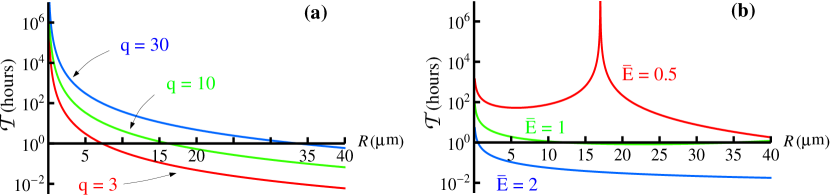
Figure 6: (color online) Jeans’ time for a homogeneous distribution of spherical particles as function of its radius $R$. The particle mobility at the interface is taken to be (see main text) $\Gamma=(3\pi R)^{-1}\;{\rm m\times s/g}$ and the interfacial surface tension is chosen as $\gamma=0.07\,{\rm N/m}$. The 2D number density $\varrho_{h}=1/({q}R)^{2}$ is parametrized in terms of ${q}$, i.e., the mean interparticle separation divided by $R$, see Eq. (24). In (a) the capillary monopole is given by Eq. (26), i.e., under the sole action of gravity, and corresponds to a vertical buoyancy force directed downwards. In (b) the capillary monopole is given by Eq. (29), i.e., the particles are under the combined action of gravity and of an external electric field. The mean interparticle separation in units of $R$ is fixed at a value ${q}=30$ and the reduced electric field $\bar{E}$ is $E/(10^{6}\,{\rm V/m})$. The divergence of ${\cal T}$ at $R\approx 15.7\,\mu\mathrm{m}$ for $\bar{E}=0.5$ corresponds to a vanishing total capillary monopole. For $\bar{E}=1$ and $\bar{E}=2$ this divergence occurs at $R\approx 63\,\mu\mathrm{m}$ and $R\approx 252\,\mu\mathrm{m}$, respectively. For this reason the curve for $\bar{E}=1$ exhibits a minimum on the scale of the figure.

IV.2 Jeans’ length

IV.2.1 Compressibility for repulsive interactions

The determination of Jeans’ length requires the specification of the equation of state of the 2D fluid of colloidal particles (see Eqs. (7) and (19)). The simplest case is that of an ideal gas, $p_{\rm ex}(\varrho)\equiv 0$; the corresponding Jeans’ length is given by

$$\frac{1}{K_{\mathrm{ideal}}}=\sqrt{\frac{\gamma T}{f^{2}\varrho}}.$$ (31)

Here the capillary monopole is only due to buoyancy so that $f=f_{\mathrm{buoy}}$ (see Eq. (26)) and $K_{\mathrm{ideal}}^{-1}\propto qR^{-2}$. This length is plotted in, c.f., Fig. 8(a) for reference. Similarly, one can consider the reference case of a 2D gas of hard disks of radius $R$ (which coincides with the radius of the spherical colloidal particles if they are half–immersed in one of the fluids). The equation of state is described well by the expression Grossman et al. (1997)

$$p=\varrho T\frac{\varrho_{c}+\varrho}{\varrho_{c}-\varrho},$$ (32)

where $\varrho_{c}:=1/(2\sqrt{3}R^{2})$ is the number density for close packing of disks in 2D. The corresponding Jeans’ length can be written as

$$\frac{1}{K}=\frac{{\cal L}(R^{2}\varrho)}{K_{\mathrm{ideal}}},$$ (33)

where $1/K_{\mathrm{ideal}}$ is Jeans’ length of an ideal gas at the same temperature and with the same number density (see Eq. (31)) and

$${\cal L}:=\frac{1}{\sqrt{\varrho T\kappa}}=\sqrt{\frac{1}{T}\frac{dp}{d\varrho}}$$ (34)

is a dimensionless function with ${\cal L}(0)=1$ which collects the deviations from the ideal gas behavior. After taking Eq. (32) into account this correction of the ideal gas behavior is a function ${\cal L}(R^{2}\varrho=q^{-2})$ solely of the dimensionless parameter ${q}$ defined in Eq. (24), which must be larger than its value ${q}_{c}=1/(R\sqrt{\varrho_{c}})\approx 1.861$ at close packing. One finds that this correction is significant actually only very close to ${q}={q}_{c}$; e.g., for ${q}=3$ one has ${\cal L}\approx 2.07$ so that in practical terms the curves in, c.f., Fig. 8(a) are applicable also for hard disks.

However, neither an ideal gas nor a gas of hard disks correspond to the generic experimental situation. Typically the particles are endowed with a soft interparticle repulsion in order to avoid coagulation brought about by attractive dispersion forces. This kind of repulsion is described by Eq. (8), where $n=3$ corresponds to the experimentally relevant situations we want to address. As stated in the context of Eq. (8), for such interaction potentials the phase diagram depends on the parameter $\zeta^{2}\varrho$ only. We have used MC simulations (details can be found in Appendix B) to compute the equation of state of this specific 2D fluid (see Fig. 7(a)), for which we are not aware of published data (compare Ref. Hoover et al. (1971) for other values of $n$ in a 3D fluid). This equation of state is valid only for $\zeta^{2}\varrho\lesssim 4.6$; beyond this value the 2D liquid freezes into a solid phase Zahn et al. (1999). Jeans’ length can be expressed again as in Eq. (33), but the function ${\cal L}$ defined by Eq. (34) is now a dimensionless function of the parameter $\zeta^{2}\varrho$ (see Fig. 7(b)). At low densities there is a relatively weak divergence, $1/K\propto 1/\sqrt{\varrho}$ (see Eq. (31)), reflecting the increase of Jeans’ length caused by a weakening of the overall capillary attraction upon dilution. At high densities close to the onset of freezing Jeans’ length increases slowly: $1/K\sim\varrho^{1/4}$ because ${\cal L}\sim(\zeta^{2}\varrho)^{3/4}$ as provided by a numerical fit and due to $1/K_{\mathrm{ideal}}\sim 1/\sqrt{\varrho}$ (see Eq. (33)).

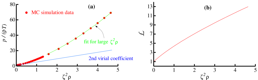
Figure 7: (color online) 2D fluid of particles interacting according to the pair potential given by Eq. (8) with $n=3$. (a) Pressure $p$ as a function of $\zeta^{2}\varrho$, so that $p/(\varrho T)\to 1$ for $\varrho\to 0$. The dots are the results from a MC simulation, while the lines correspond to the approximation of the equation of state up to the second term in the virial expansion, $p\approx\varrho T[1+(\pi/2)\Gamma(1/3)\zeta^{2}\varrho]$, valid for low densities, and to the numerical fit $p\approx\varrho T[3+6.6(\zeta^{2}\varrho)^{3/2}]$, valid for large densities. Note that this latter fitting function corresponds to the equation of state of an harmonic solid of soft particles interacting with the pair potential $r^{-3}$ Speedy (2003). We have found that in good approximation this equation of state also holds for the corresponding high–density fluid phase. For $\zeta^{2}\varrho\gtrsim 4.6$ the fluid freezes. (b) The dimensionless function ${\cal L}$ given by Eq. (34) which characterizes Jeans’ length (Eq. (33)).

IV.2.2 Repulsion between electrically charged particles

A common way of implementing the interparticle repulsion is to use electrically charged particles or, more frequently, cover the particle surfaces with chemical groups which dissociate in water. (Even then, the repulsion is long–ranged if the adjacent fluid phase is a dielectric Domínguez et al. (2008).) The repulsion is described by Eq. (8) with $n=3$ and Frydel et al. (2007)

$$\left(\frac{\zeta}{R}\right)^{3}=2\frac{\epsilon_{1}}{\epsilon_{2}}\frac{R}{\lambda_{B}}\left[(1+\cos\theta)\,g_{\rm lin}\,\ln\left(\frac{4\pi\sigma_{c}\lambda_{B}}{e\kappa_{D}}\right)\right]^{2}.$$ (35)

Here, $1<\epsilon_{1}\lesssim 3$ and $\epsilon_{2}\approx 80$ are the dielectric constants of air (or oil) and water, respectively, $\lambda_{B}\approx 0.7\,{\rm nm}$ is the Bjerrum length in water at room temperature, $\kappa_{D}^{-1}\lesssim 1\,\mu{\rm m}$ is the Debye screening length in water, $e$ is the positive elementary charge, $\sigma_{\rm c}$ is the charge density at the surfaces of the particles in contact with water, $\theta$ is the contact angle at the particle–interface contact line, and $0.1\lesssim g_{\rm lin}(\theta,\kappa_{D})\lesssim 1$ is a factor of geometrical origin. For strongly charged colloids one typically has $\sigma_{c}\sim 0.5\,e/{\rm nm^{2}}$, while water with a salt concentration above $10^{-2}\,$M has a screening length $\kappa_{D}^{-1}$ below a few nanometers. Under these conditions, the factor $[(1+\cos\theta)\,g_{\rm lin}\,\ln(4\pi\sigma_{c}\lambda_{B}/e\kappa_{D})]^{2}$ is of the order of the unity, and in the following quantitative estimates we replace it by 1. Furthermore, we take $\epsilon_{2}/\epsilon_{1}\approx 40$ as appropriate for an oil–water interface. For these values of the parameters one has

$$\zeta^{2}\varrho\approx\frac{17.22}{{q}^{2}}\left(\frac{R}{\mu{\rm m}}\right)^{2/3}.$$ (36)

For this expression Fig. 8 shows Jeans’ length $1/K$ (see Eq. (33)) as a function of the particle radius $R$ for various values ${q}$ of the mean interparticle separation in units of $R$.

IV.2.3 Repulsion between induced electric dipoles

In the experiment described in Ref. Aubry et al. (2008), the dipoles induced by the external electric field give rise to an interparticle repulsion described also by Eq. (8) with $n=3$ and

$$\left(\frac{\zeta}{R}\right)^{3}=-\frac{\varepsilon_{0}R^{3}E^{2}}{3T}(\epsilon_{2}+\epsilon_{1})\psi,$$ (37)

where the factor $\psi$ depends on the dielectric constants and the height of the particle at the interface (see Fig. 9 in Ref. Aubry and Singh (2008), where the factor $\psi$ is called $f_{d}$). For the experiment in Ref. Aubry et al. (2008) one has $\epsilon_{1}=1$, $\epsilon_{2}\approx 2.87$, and $\psi\approx-0.019$ so that

$$\zeta^{2}\varrho\approx\frac{14.00}{{q}^{2}}\left(\frac{E}{10^{6}\,{\rm V/m}}\right)^{4/3}\left(\frac{R}{\mu{\rm m}}\right)^{2}$$ (38)

at room temperature. For this expression, Fig. 9 shows Jeans’ length $1/K$ (see Eq. (33)) as a function of the particle radius $R$.

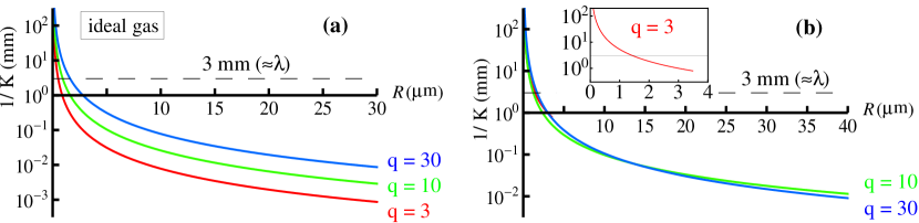
Figure 8: (color online) Jeans’ length for buoyancy induced monopoles (see Eq. (26)) and (a) for the ideal gas equation of state (see Eq. (31)) (also valid for a gas of hard disks, see the discussion after Eq. (34)), or (b) for the equation of state corresponding to dipolar repulsion between electrically charged particles estimated by taking charge renormalization into account (see Eqs. (33) and (36)). ${q}$ is the mean interparticle separation in units of $R$ (Eq. (24)). The dashed, horizontal line indicates the value of $3\;$mm corresponding to a typical value of the capillary length $\lambda$. Capillary–induced clustering is possible below this line (see Fig. 3). (The curve for ${q}=3$ in the inset stops at $R\approx 4\,\mu$m due to the onset of freezing.)

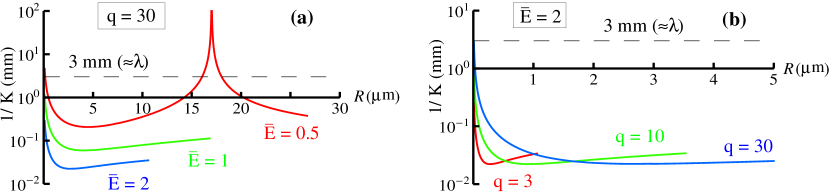
Figure 9: (color online) Jeans’ length $1/K$ for buoyancy and electric field induced monopoles (see Eq. (29)) and for the equation of state corresponding to electric field induced dipolar repulsion (see Eqs. (33) and (38)). In (a) Jeans’ length is reported for various values $\bar{E}$ of the electric field in units of $10^{6}\,\mathrm{V/m}$ and for a fixed mean interparticle separation ${q}=30$ (in units of $R$). The divergence of $1/K$ at $R\approx 15.7\,\mu\mathrm{m}$ for $\bar{E}=0.5$ corresponds to a vanishing total capillary monopole. In (b) various values of ${q}$ for a fixed electric field $E=2\times 10^{6}\,\mathrm{V/m}$ are studied. The dashed, horizontal line indicates the value of $3\;$mm corresponding to a typical value of the capillary length $\lambda$. Capillary–induced clustering is possible below this line (see Fig. 3). (When a curve stops, it does so at the corresponding onset of freezing.)

IV.2.4 Repulsion between induced magnetic dipoles

In the experimental setup with superparamagnetic particles of susceptibility $\chi_{\mathrm{m}}$, an external magnetic field $H$ induces a magnetic moment, which in a spherical particle of radius $R$ is given by

$$m=\frac{4\pi}{3}R^{3}\chi_{\mathrm{m}}H.$$ (39)

In turn this leads to a dipolar repulsion described also by Eq. (8) with $n=3$ and

$$\zeta^{3}=\frac{\mu_{0}m^{2}}{4\pi T}.$$ (40)

In the experiments described in Refs. Zahn et al. (1997, 1999) the susceptibility is $\chi_{\mathrm{m}}\approx 1.7$ and the magnetic field $H$ ranges typically between $10^{2}\,$A/m and $10^{3}\,$A/m, which corresponds to

$$\zeta^{2}\varrho\approx\frac{5.31}{{q}^{2}}\left(\frac{H}{10^{2}\,{\rm A/m}}\right)^{4/3}\left(\frac{R}{\mu{\rm m}}\right)^{2}$$ (41)

at room temperature. (For comparison, Earth’s magnetic field has a strength of about $40\,$A/m and sets a lower bound on the value of $H$ achievable in the laboratory, unless the magnetic field is generated in a specific configuration so as to counterbalance Earth’s field.) Figure 10 shows Jeans’ length $1/K$ (see Eq. (33)) as a function of the particle radius $R$. (As remarked in Subsec. IV.1.3, the contribution to the capillary monopole due to the magnetic field is negligible.)

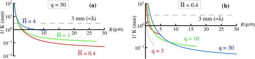
Figure 10: (color online) Jeans’ length $1/K$ for buoyancy induced monopoles (see Eq. (26)) and for the equation of state corresponding to magnetic field induced dipolar repulsion (see Eqs. (33) and (41)). In (a) various values of the reduced magnetic field $\bar{H}=H/(10^{2}\,\mathrm{A/m})$ are studied for a fixed mean interparticle separation ${q}=30$ (in units of $R$). In (b) Jeans’ length is shown for various values of ${q}$ at the fixed field strength $H=40\,\mathrm{A/m}$ corresponding to Earth’s magnetic field. The dashed, horizontal line indicates the value of $3\;$mm corresponding to a typical value of the capillary length $\lambda$. Capillary–induced clustering is possible below this line (see Fig. 3). (When a curve stops, it does so at the corresponding onset of freezing.)

V Discussion

Our results show that there is a range of parameters for presently accessible experimental setups which allows one to observe the instability of colloidal monolayers at fluid interfaces driven by capillary attraction: particle size in the micrometer range, Jeans’ length well below the capillary length, and Jeans’ time ranging from minutes to weeks. This provides theoretical evidence for the possibility that capillary attraction can lead to relevant aggregation effects at submillimeter length scales in spite of its relative weakness at the mean distances between the particles.

In view of the estimates derived in Sec. IV, it is conceivable that many experiments carried out so far happen to operate in the range of parameters within which the homogeneous configuration is stable against capillary–induced clustering. For charge–stabilized colloids (see Fig. 8(b)) the particles employed experimentally are usually too small (not larger than a few micrometers). In the experiments carried out with superparamagnetic particles Zahn et al. (1999, 1997) (see Fig. 10), the particles are too small ($R\approx 2.5\,\mu$m), the magnetic fields too large, and it is likely that the capillary monopole is also too small (because the particles are completely submerged in water, albeit close to the interface). In Ref. Aubry et al. (2008), which reports experiments in an electric field with spherical particles ranging in radius between $2\,\mu\mathrm{m}$ and $77\,\mu\mathrm{m}$, there is a brief remark on the clustering of particles by capillary attraction in the absence of the electric field: In these experiments the particles were in close contact in the clustered states (with a mean interparticle separation, as inferred from the photographs, of ${q}\lesssim 2$ (in units of $R$)), corresponding to states in the solid phase. The lack of information on the pre-clustered mean particle density renders our results in the fluid phase of limited use for the comparison with the experimental observations. Nevertheless, assuming a hard–disk equation of state for the particles in the absence of the electric field, Fig. 8(a) indicates the formation of a cluster for the range of particle sizes employed in this experiment, with collapse times spanning several orders of magnitude (see Fig. 6(a)). The only quantitative experimental studies of the clustering instability we are aware of which do provide data amenable to comparison with our calculations can be found in Refs. Hórvölgyi et al. (1994); Vincze et al. (2001). According to the interpretation of those authors, temperature inhomogeneities at the interface set the particles in tomotion, the clustering of which is initially driven by capillary forces; further restructuring of the emerging formations inside the clusters involves short–ranged forces. This latter feature is beyond the scope of our model and we are not in a position to judge the influence of the temperature inhomogeneities. We simply note that, for buoyant particles of size $R\approx 35\,\mu\mathrm{m}$ spread with an initial areal density corresponding to ${q}\approx 10$ Vincze et al. (2001), Fig. 8 predicts indeed capillary–induced clustering and Fig. 6(a) yields Jeans’ time of the order of a few minutes, in good agreement with the reported characteristic times (see Fig. 3 of Ref. Vincze et al. (2001)). In summary, according to our estimates it seems to be possible to perform experiments within an appropriate range of controllable physical parameters which would promote the occurrence of the capillary–induced instability in a variety of conditions and which would allow the systematic study of its dynamical evolution.

The tempting question arises whether the so far unexplained interparticle attraction and the ensuing micron–sized clusters we referred to in Sec. I and which are reported by various groups can be understood within the physical picture we have presented: a cluster would be held together against repulsion and thermal diffusion by the collective capillary attraction and it would be the final, equilibrium state of a capillary–induced collapse. The answer is negative. First, there is a dynamical counterargument based on our theoretical finding that a capillary–induced clustering would require the almost simultaneous collapse of spontaneous density fluctuations of all sizes (see Eq. (23)): shortly after the formation of the actually observed micrometer–sized clusters, there should also arise many other clusters of larger sizes and all particles would eventually gather in a single, large cluster. Such a phenomenon has not been reported. Secondly, there is a static counterargument based on the qualitative reasoning put forward in Subsec. II.1, which states that the equilibrium size of the cluster is of the order of Jeans’ length associated with the cluster density: as follows from Fig. 8, there is no range of realistic values of the parameters for which Jeans’ length is of the order of the observed cluster size, typically tens of micrometers at most, i.e., less than $10^{-2}\,\mathrm{mm}$. In other words, the observed clusters consist of too few particles in order to be able to build up a collective capillary attraction of relevant strength.

One has also observed colloidal crystals spanning the whole system, which has a typical size $L$ in the millimeter or centimeter range, i.e., comparable with the capillary length $\lambda$ or somewhat larger (see, e.g., Ref. Smalyukh et al. (2004); Aubry et al. (2008)). One could try to explain this particle distribution as a very large cluster, self–confined by its own capillary attraction. Within our model, this would correspond to a clustered state characterized by a cluster Jeans’ length $L_{J}$ of the order of $\lambda$ (see Subsec. II.1). Although our results pertain to the fluid phase of the 2D colloid, one could nevertheless use them as rough estimates for the solid phase, given the relatively weak squared–root dependence of Jeans’ length on the compressibility (see Eq. (19)). Thus, Figs. 8 and 9 provide evidence that the condition $L_{J}\sim\lambda$ could be easily satisfied. Actually, Ref. Aubry et al. (2008) mentions briefly the interpretation of the occurrence of large clusters as being due to capillary attraction.

Recently, Pergamenshchik (2009) has correctly pointed out the enhancement of the pairwise capillary attraction due to a collective effect involving many particles. His work addresses only the equilibrium configuration of clusters of a size much larger than the capillary length and in the solid phase. His somewhat involved calculations can be put in our present context as follows: The solid phase is described effectively by the equation of state of a harmonic solid of soft spheres, which for the repulsive potential given by Eq. (8) corresponds to a pressure $p(\varrho)\propto\varrho^{1+(n/2)}$ at high densities Speedy (2003). Integration of the equilibrium condition expressed by Eq. (11) yields $\varrho\propto(U-U_{0})^{2/n}$, where $U_{0}$ is an integration constant. Inserting this result into Eq. (9) one recovers Eq. (39) of Ref. Pergamenshchik (2009), which is his central result (notice that the exponent $n$ in our notation (see Eq. (8)) corresponds to $n-1$ in Pergamenshchik’s notation (see Eq. (31) in Ref. Pergamenshchik (2009))). These considerations show that the approach used in Ref. Pergamenshchik (2009) is contained in the theoretical framework presented here.

However, in view of the discussion given above his claims that such a collective effect explains the clusters observed so far in experiments appear to be unsubstantiated. First, the analysis of an infinitely extended cluster misses the explicit size–dependence of the capillary energy (see Eq. (4)), which makes his results unapplicable to small clusters. Secondly, his actual application of these results to experiments considers only either an ideal gas or a gas of hard disks. As we have shown in our analysis, these two models do not give rise to significant differences among them but both represent inadequate approximations for generic conditions in typical experimental systems. This difference can be understood in terms of the non–capillary contribution to the energy (see Eq. (5)): an ideal gas or a gas of hard disks contributes kinetic energy only, which is of the order of the thermal energy $T$ per particle (in units of the Boltzmann constant), whereas for the interparticle potential given by Eq. (8), the virial theorem yields an energy per particle $e_{\mathrm{short}}/T=1+(2/n)(p/(\varrho T)-1)$, which according to Fig. 7(a) can be at least $\approx 100T$ in the solid phase.

The analogy of the model presented here with the 2D evolution of a self–gravitating fluid is not complete: the capillary attraction is, unlike gravity, screened beyond the capillary length, and the temporal evolution is ruled by an overdamped dynamics (see Eq. (13), amended in general with the effect of hydrodynamic interactions at sufficiently high densities) rather than by the inertial, Newtonian dynamics for gravitating particles. This poses the question as to which extent the gravitational phenomenology can be reproduced by colloids at a fluid interface. Our study provides a partial answer, in that it demonstrates the existence of a clustering instability which is analogous to Jeans’ instability. But this is still far from being a complete and systematic comparison, which could provide the tempting picture of the feasibility to study “cosmology in a Petri dish”. In this context, it would be interesting to investigate the equilibrium configuration of clusters and their stability beyond the simple qualitative analysis we have presented in Subsec. II.1, i.e., by solving Eqs. (9) and (11). Such a study would be complementary to the analysis of the dynamical aspects we have addressed here. The form of the capillary attraction also leads to a possible analogy with two–dimensional vortices, the similarity of which with a self–gravitating system is also well known. However, how deep and useful this latter analogy can be is still a matter of study (see, e.g., Ref. Chavanis (2002) and references therein).

VI Conclusion

We have presented a mean–field model for the evolution of the density of colloidal particles at a fluid interface driven by its own capillary attraction. In spite of the weakness of the capillary interaction at the mean distance between particles, its non-integrable character at submillimeter length scales enhances its effect on the evolution of collective modes. We have demonstrated that if the characteristic Jeans’ length (see Eq. (19)) of a homogeneous distribution is sufficiently small (see Fig. 3) the system can be unstable with respect to long–wavelength density perturbations under the action of capillary attraction (see Fig. 4). Beyond this linear stability analysis, we have also solved the nonlinear evolution of radially symmetric density perturbations (see Fig. 11) in the so-called cold–collapse approximation (within which the dynamics is driven by capillary attraction only) (see Figs. 12 – 14), which predicts a typical time of collapse of the order of Jeans’ time (see Eqs. (19) and (64)). By computing Jeans’ length and time for presently accessible experimental setups we obtain clear predictions about the range of parameter values within which the instability could be observed. Jeans’ time (see Fig. 6) depends on the strength of the capillary monopole. To this end we have considered the monopole to be induced either by buoyancy or by an external electric field. Jeans’ length depends additionally on the equation of state of the 2D gas via its compressibility. In this context we have studied an ideal gas (see Fig. 8(a)) and systems with a dipolar interparticle repulsion (see Eq. (8) for $n=3$) induced either by electric charges on the particles (see Fig. 8(b)), an external electric field (see Fig. 9), or an external magnetic field (see Fig. 10). In most experiments performed so far, the physical parameters lie in the region of stability, but they appear to be easily tunable into the instability regime. The relatively weak dependence of Jeans’ length on the equation of state (via the square root of the compressibility, see Eq. (19)), renders the capillary monopole to be a possibly more convenient parameter for tuning Jeans’ length and time. Experiments with 2D colloids exposed to an external electric field seem particularly promising in this respect, because the field provides a simple way of controlling the vertical pull on the particles generating in turn the mediating interfacial deformation. Similarly, a vertical force on superparamagnetic particles in an external magnetic field could be created and controlled via gradients of the magnetic field which pull on the induced magnetic moments.

Appendix A Functional formulation

The mathematical model defined by Eqs. (9) and (14) can be reformulated in terms of the functional ${\cal F}[\varrho,U]={\cal F}_{\rm cap}+{\cal F}_{\rm gas}+{\cal F}_{\rm inter}$, consisting of three contributions. The first one is related to the capillary deformation in the small–deformation limit:

$${\cal F}_{\rm cap}:=\frac{1}{2}\gamma\int dA\;\left[|\nabla U|^{2}+\left(\frac{U}{\lambda}\right)^{2}\right].$$ (42)

The second term is the free energy functional (within local approximations) of the 2D gas of particles,

$${\cal F}_{\rm gas}:=\int dA\;\mathsf{f_{gas}}(T,\varrho),\qquad\mathsf{f_{gas}}(T,\varrho)=T\varrho[\ln(\Lambda^{2}\varrho)-1]+\mathsf{f_{ex}}(T,\varrho),$$ (43)

where the free energy density $\mathsf{f_{gas}}(T,\varrho)$ is the sum of the ideal gas contribution ($\Lambda$ is de Broglie’s thermal length) and the excess free energy $\mathsf{f_{ex}}$ due to the repulsive short–ranged forces. Finally, the third term represents the interaction between the particles and the interfacial deformation:

$${\cal F}_{\rm inter}:=-f\int dA\;\varrho\,U.$$ (44)

The mean–field equation (9) for the interfacial deformation follows from the extremal condition

$$\frac{\delta{\cal F}}{\delta U({\bf r})}=0,$$ (45)

while the diffusion equation (14) can be expressed in terms of a relaxation–type dynamics,

$$\frac{\partial\varrho}{\partial t}=\Gamma\nabla\cdot\left[\varrho\nabla\frac{\delta{\cal F}}{\delta\varrho({\bf r})}\right],$$ (46)

upon using the thermodynamical identity

$$p(\varrho)=\varrho^{2}\frac{\partial}{\partial\varrho}\left(\frac{\mathsf{f_{gas}}(T,\varrho)}{\varrho}\right)_{T}\qquad\Rightarrow\qquad\nabla p=\varrho\nabla\left(\frac{\partial\mathsf{f_{gas}}}{\partial\varrho}\right)\quad\textrm{at constant }T.$$ (47)

In principle, ${\cal F}$ can be viewed as an effective functional reformulation of the problem, although it can be associated with an actual free–energy functional for the physical system. In this case, the mean–field approximation enters via the simplified form of Eq. (44): a complete description of the particle–interface interaction should take into account the finite size of the particles (rather than a point capillary monopole), their shape, the corresponding surface energies (see, e.g., the free–energy functional introduced in Ref. Oettel et al. (2005a)), and a thermal noise contribution to Eq. (46). A procedure for incorporating the hydrodynamic interactions into the functional formulation has been proposed recently in Ref. Rex and Löwen (2009).

Appendix B Equation of state from numerical simulations

We investigate a two–dimensional fluid governed by the pair potential given by the power law in Eq. (8) with $n=3$. The equation of state of such a fluid depends only on the dimensionless parameter $\zeta^{2}\rho$ Hoover et al. (1971). Thus it is advantageous to introduce the new length scale $\tilde{\sigma}=1/\sqrt{\rho}$ such that

$$\frac{v_{\mathrm{rep}}(d)}{T}=(\zeta^{2}\rho)^{3/2}\left(\frac{\tilde{\sigma}}{d}\right)^{3}\;.$$ (48)

In the simulation one fixes $\tilde{\sigma}$ as the unit of length and varies the prefactor $(\zeta^{2}\rho)^{3/2}$. The pressure can be determined from the virial expression

$$p=\rho T+\frac{1}{2A}\langle\sum_{i<j}{\bf f}({\bf r}_{i}-{\bf r}_{j})\cdot({\bf r}_{i}-{\bf r}_{j})\rangle$$ (49)

where $A$ is the area of the simulation box and ${\bf f}=-\nabla v_{\mathrm{rep}}$ is the interparticle force. In our case

$$\sum_{i<j}{\bf f}({\bf r}_{i}-{\bf r}_{j})\cdot({\bf r}_{i}-{\bf r}_{j})=3\sum_{i<j}v_{\mathrm{rep}}({\bf r}_{i}-{\bf r}_{j})\;,$$ (50)

so that the pressure is related to the excess internal energy $U^{\rm ex}$ of the fluid according to

$$p=\rho T+\frac{3}{2}\frac{U^{\rm ex}}{A}\;.$$ (51)

The simulations have been carried out with $N=400$ particles in a square simulation box with reduced side length $L=20$ (in units of $\tilde{\sigma}$). Periodic boundary conditions were applied. The internal energy of a given configuration of the $N$ particles was obtained by summing over $(2l+1)\times(2l+1)$ boxes (i.e., the central simulation box plus image boxes around it) because the pair potential decays slowly (we chose $l=3$). $U^{\rm ex}$ was determined as an average over $10^{4}$ sweeps (one sweep corresponds to attempted moves for every particle in the box). The instantaneous internal energy was determined for each sweep once.

Appendix C Radially symmetric cold collapse

Figure 11: Evolution of a radially symmetric enhanced density. An infinitesimally thin ring of particles of initial radius $R_{0}$ collapses to a ring of radius $R(t)<R_{0}$ at a time $t>0$. By construction the ring follows the motion of its particles and it can be identified by its Lagrangian radial coordinate $R_{0}$ (and $R(t)$ is the Eulerian radial coordinate of the ring). Therefore, the number of particles inside the disk encircled by the ring is constant if different rings do not cross (one cannot exclude a priori that a ring is overtaken by another one because different rings may collapse with different speeds).

C.1 General dynamics of radially symmetric cold collapse

A homogeneous configuration is characterized by a density $\varrho_{h}$ and a mean–field interfacial deformation $U_{h}=f\lambda^{2}\varrho_{h}/\gamma$ given by Eq. (9). We study the evolution of a radially symmetric density perturbation so that

$$\varrho({\bf r},t)=\varrho_{h}+\delta\varrho(r,t).$$ (52)

The perturbation $\delta U$ of the interfacial deformation is given by the solution of Eq. (16). (Note that this latter equation is not a linearized approximation requiring $\delta\varrho$ and $\delta U$ to be small, because Eq. (9) is linear; the nonlinearity of the dynamics enters via Eq. (14).) We consider a sufficiently localized density perturbation, i.e., $\delta\varrho$ vanishes sufficiently fast at infinity, so that the solution in the limit of large capillary length $\lambda$ follows immediately from the gravitational analogy: the capillary force on a particle is (compare Eq. (3))

$$f\nabla(\delta U)=-\frac{f^{2}\,\delta N(r,t)}{2\pi\gamma r}{\bf e}_{r},\qquad(\lambda\to\infty)$$ (53)

where

$$\delta N(r,t):=2\pi\int_{0}^{r}ds\,s\,\delta\varrho(s,t)$$ (54)

is the excess number of particles in a disk of radius $r$ concentric with the perturbation. The density field follows from solving Eqs. (12)–(14), which in the cold collapse approximation, i.e., after neglecting any force other than the capillary attraction, reduce to (see Eq. (53))

$$\frac{\partial(\delta\varrho)}{\partial t}=-\nabla\cdot({\bf v}\varrho),$$ (55)

$${\bf v}=\Gamma f\nabla(\delta U).$$ (56)

An exact solution is possible by resorting to a description of the flow in terms of Lagrangian coordinates. Consider the thin ring of radius $R(t;R_{0})$ formed by the particles which were initially ($t=0$) at a distance $R_{0}$ from the center, i.e., the ring is defined through its Lagrangian radial coordinate $R_{0}$ (see Fig. 11). Equation (55) implies that the number of particles encircled by the ring is conserved:

$$N(R,t):=2\pi\int_{0}^{R}ds\,s\,\varrho(s,t)=N_{0}(R_{0})=2\pi\int_{0}^{R_{0}}ds\,s\,\varrho_{0}(s),$$ (57)

where $N_{0}(R_{0})$ is the initial number of particles encircled by the ring of radius $R_{0}$. (Since, at fixed $t$, $N(R,t)$ is a monotonous function of $R$, Eq. (57) provides a relation $R_{0}=R_{0}(t;R)$ which can be inverted, $R=R(t;R_{0})$, with the geometrical meaning “radius of the ring at time $t$ which had a radius $R_{0}$ at time $t=0$”.) This expression allows an explicit computation of the density field,

$$\varrho(R,t)=\frac{1}{2\pi R}\left.\frac{\partial N}{\partial R}\right|_{t}=\frac{1}{2\pi R}\frac{dN_{0}}{dR_{0}}\left.\frac{\partial R_{0}}{\partial R}\right|_{t}=\frac{R_{0}}{R}\varrho_{0}(R_{0})\left.\frac{\partial R_{0}}{\partial R}\right|_{t}.$$ (58)

The evolution of the ring radius $R(t;R_{0})$ is determined by the flow velocity,

$$\left.\frac{\partial R}{\partial t}\right|_{R_{0}}{\bf e}_{r}={\bf v},$$ (59)

with ${\bf v}$ given by Eq. (56). By inserting the solution (53) and making use of particle conservation, $\delta N(R,t)=N(R,t)-\pi R^{2}\varrho_{h}=N_{0}(R_{0})-\pi R^{2}\varrho_{h}$ (see Eq. (57)), one finally arrives at an ordinary, first–order differential equation for $R(t;R_{0})$:

$$\left.\frac{\partial R}{\partial t}\right|_{R_{0}}=\left.\Gamma f{\bf e}_{r}\cdot\nabla(\delta U)\right|_{r=R}=-\frac{f^{2}\Gamma}{2\pi\gamma R}[N_{0}(R_{0})-\pi R^{2}\varrho_{h}].$$ (60)

In terms of the characteristic time ${{\cal T}}=\gamma/(\Gamma f^{2}\varrho_{h})$ of the homogeneous background configuration (see Eq. (19)) one can write

$${{\cal T}}\left.\frac{\partial}{\partial t}\left(\frac{R}{R_{0}}\right)^{2}\right|_{R_{0}}=\left(\frac{R}{R_{0}}\right)^{2}-\frac{\hat{\varrho}_{0}}{\varrho_{h}},$$ (61)

where

$$\hat{\varrho}_{0}(R_{0}):=\frac{N_{0}(R_{0})}{\pi R_{0}^{2}}$$ (62)

is the average initial density of the disk of radius $R_{0}$. The solution of this equation with the boundary condition $R(t=0;R_{0})=R_{0}$ reads

$$R(t;R_{0})=R_{0}\sqrt{\frac{\hat{\varrho}_{0}}{\varrho_{h}}+\left(1-\frac{\hat{\varrho}_{0}}{\varrho_{h}}\right){\rm e}^{t/{{\cal T}}}}.$$ (63)

Figure 12 plots the evolution $R(t)$ for the two possible, qualitatively different cases: If $\varrho_{h}>\hat{\varrho}_{0}$ the ring expands. (When $R$ reaches $\lambda$ the model ceases to be valid because then one must take into account the screening of the capillary interaction neglected in Eq. (53).) In the other case, $\varrho_{h}<\hat{\varrho}_{0}$, the ring contracts and $R=0$ is reached at a time

$${{\cal T}}_{\rm coll}=-{{\cal T}}\ln\left(1-\frac{\varrho_{h}}{\hat{\varrho}_{0}}\right).$$ (64)

Obviously, true collapse is prevented by a finite compressibility which has been neglected in the above calculations (see Eq. (56)) and a spatially extended equilibrium configuration will emerge. However, the unambiguos identification of a ring by its Lagrangian radius $R_{0}$ would no longer hold if two different rings would coincide before the collapse at the center (a phenomenon customarily called shell crossing in 3D in the cosmological literature). If this would happen, a density singularity would appear, maybe regularized by the repulsive forces present. It can be shown that a sufficient and necessary condition to avoid ring crossing is that the time of collapse ${{\cal T}}_{\rm coll}(R_{0})$ of the ring characterized by its initial radius $R_{0}$ grows with this radius. In view of Eq. (64), this is equivalent to the condition

$$\frac{d\hat{\varrho}_{0}}{dR_{0}}\leq 0,$$ (65)

i.e., the initial perturbation inside a disk looks more and more rarefied as the disk radius is taken larger and larger.

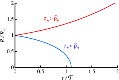
Figure 12: (color online) Evolution in time of the radius $R(t;R_{0})$ of a circular ring during cold collapse (Eq. (63)). Two qualitatively different cases (expansion and collapse) can be distinguished depending on the initial average density $\hat{\varrho}_{0}$ in the area encircled by the ring compared to the background density $\varrho_{h}$. The curves correspond to $\hat{\varrho}_{0}/\varrho_{h}=0.5$ for expansion and $\hat{\varrho}_{0}/\varrho_{h}=1.5$ for collapse.

C.2 Example of cold collapse for a steplike overdensity

As a simple application of these results we consider a top–hat enhanced density, described by the initial profile

$$\varrho_{0}(r)=\varrho_{h}+\delta\varrho_{0}\,\Theta(L_{0}-r)=\left\{\begin{array}[c]{cc}\varrho_{h}+\delta\varrho_{0},&r<L_{0}\\ \varrho_{h},&L_{0}<r\end{array}\right.\qquad(\delta\varrho_{0}>0),$$ (66)

where $\Theta(x)$ is Heavyside’s step function. We assume that the initial radius fulfills $K^{-1}\ll L_{0}\ll\lambda$, so that the simplifying assumptions of the previous calculations hold. For this profile, one has (Eq. (62))

$$\hat{\varrho}_{0}(R_{0})=\left\{\begin{array}[c]{cc}\varrho_{h}+\delta\varrho_{0},&R_{0}\leq L_{0}\\ &\\ \displaystyle\varrho_{h}+\left(\frac{L_{0}}{R_{0}}\right)^{2}\delta\varrho_{0},&L_{0}<R_{0},\end{array}\right.$$ (67)

so that $\varrho_{h}<\hat{\varrho}_{0}$ and, according to Fig. 12, there is a collapse for all $L_{0}>0$. The time of collapse (see Eq. (64))

$${{\cal T}}_{\rm coll}(R_{0})={{\cal T}}\ln\left\{1+\frac{\varrho_{h}}{\delta\varrho_{0}}\left[\Theta(L_{0}-R_{0})+\left(\frac{R_{0}}{L_{0}}\right)^{2}\Theta(R_{0}-L_{0})\right]\right\}$$ (68)

is plotted in Fig. 13: the whole interior of the overdensity ($R_{0}<L_{0}$) collapses simultaneously, i.e., ${{\cal T}}_{\mathrm{coll}}$ is independent of $R_{0}$. The evolution of the density profile $\varrho(r,t)$ follows from Eqs. (58) and (66): by inserting Eq. (67) into Eq. (63) one obtains upon differentiation

$$\left.\frac{R}{R_{0}}\frac{\partial R}{\partial R_{0}}\right|_{t}=\left\{\begin{array}[c]{cc}(R/R_{0})^{2},&R_{0}<L_{0}\\ 1,&L_{0}<R_{0}\end{array}\right.$$ (69)

so that the density profile preserves the top–hat shape during the evolution (see Fig. 14):

$$\varrho(r,t)=\left\{\begin{array}[c]{cc}\displaystyle\left[\frac{L_{0}}{L(t)}\right]^{2}(\varrho_{h}+\delta\varrho_{0}),&r<L(t)\\ &\\ \varrho_{h},&L(t)<r\end{array}\right.$$ (70)

where

$$L(t)=L_{0}\sqrt{\frac{\varrho_{h}+\delta\varrho_{0}}{\varrho_{h}}\left[1-{\rm e}^{(t-{{\cal T}}_{\rm coll})/{{\cal T}}}\right]}$$ (71)

is the time–dependent radius of the region with enhanced density, i.e., Eq. (63) evaluated for the particular case $R_{0}=L_{0}$ by using Eqs. (64) and (67). Consistently with this geometrical meaning, $L(t)$ vanishes at the time of collapse $t={{\cal T}}_{\mathrm{coll}}(R_{0}=L_{0})$ of this region, as given by Eq. (68). (Upon deriving Eq. (70) one notices that the region with enhanced density can be characterized by the inequality $R_{0}<L_{0}$ or equivalently by $r<L(t)$, since $r=R(t;R_{0})$.) The sharp jump in the density profile is of course an idealization in the limit of infinite compressibility. The jump would be actually smoothed out by the pressure forces, but on a length scale much smaller than the spatial extension of the density enhancement.

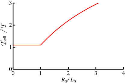
Figure 13: (color online) Dependence of the time of collapse on the ring radius for a top–hat enhanced density distribution. The plot corresponds to the case $\delta\varrho_{0}=0.5\varrho_{h}$ (see Eq. (68)). The time scale is set by Jeans’ time ${{\cal T}}$ (Eq. (19)).

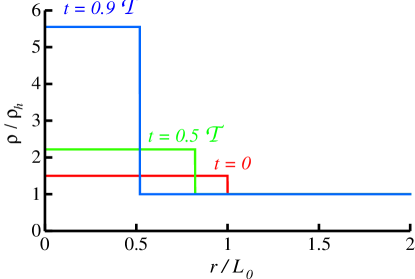
Figure 14: (color online) Time evolution of the density profile of an initial top–hat enhanced density distribution (Eq. (70)). The plot corresponds to $\delta\varrho_{0}=0.5\varrho_{h}$. The time scale is set by Jeans’ time ${{\cal T}}$ (Eq. (19)).

As the perturbation is compressed, in the 2D fluid the pressure increases until it is able to counterbalance the total capillary force and stop the collapse. One can derive a simple estimate for the smallest size $L_{\mathrm{min}}$ of the compressed cluster as follows: at the maximum density $\varrho_{\rm max}\gg\varrho_{h}$, corresponding to a cluster radius $L_{\rm min}\ll L_{0}\ll\lambda$, a total pressure force of the order of $F_{\rm p}\sim 2\pi L_{\rm min}p(\varrho_{\rm max})$ opposes the total compressing capillary force, which is of the order of $F_{\rm cap}\sim(fN)^{2}/(2\pi\gamma L_{\rm min})$. (The cluster consists of $\approx N$ particles and the capillary force on each of them is given by Eq. (53) with $\delta N=\pi L_{\rm min}^{2}(\varrho_{\rm max}-\varrho_{h})\approx N$ due to $\varrho_{\rm max}\gg\varrho_{h}$.) Therefore, in equilibrium $F_{\rm p}\sim F_{\rm cap}$, giving the relationship

$$p(\varrho_{\rm max})\sim\frac{(fL_{\rm min}\varrho_{\rm max})^{2}}{4\gamma}.$$ (72)

Upon introducing Jeans’ length $K_{\rm cluster}^{-1}$ of the cluster, i.e., Eq. (19) evaluated at the cluster average density $\varrho_{\rm max}$, this can be rewritten as

$$(K_{\rm cluster}L_{\rm min})^{2}\sim 4p(\varrho_{\rm max})\kappa(\varrho_{\rm max}).$$ (73)

For polytropic equations of state, $p(\varrho)\propto\varrho^{z}$, or more generally for a simple fluid far from any phase transition, the right hand side of this expression is typically of the order of unity, so that the final equilibrium size of the cluster will be comparable to its Jeans’ length. This rough estimate agrees with the results obtained from the qualitative reasoning given in Subsec. II.1.

References

- Pieranski (1980) P. Pieranski, Phys. Rev. Lett. 45, 569 (1980).
- Chateau and Pitois (2003) X. Chateau and O. Pitois, J. Coll. Interface Sci. 259, 346 (2003).
- Zahn et al. (1999) K. Zahn, R. Lenke, and G. Maret, Phys. Rev. Lett. 82, 2721 (1999).
- Velikov and Velev (2006) K. P. Velikov and O. D. Velev, Colloidal Particles at Liquid Interfaces (Cambridge University Press, 2006), pp. 225–297.
- Oettel and Dietrich (2008) M. Oettel and S. Dietrich, Langmuir 24, 1425 (2008).
- Kleman and Lavrentovich (2003) M. Kleman and O. D. Lavrentovich, Soft Matter Physics (Springer, New York, 2003).
- Hurd (1985) A. J. Hurd, J. Phys. A: Math. Gen. 18, L1055 (1985).
- Frydel et al. (2007) D. Frydel, S. Dietrich, and M. Oettel, Phys. Rev. Lett. 99, 118302 (2007).
- Domínguez et al. (2008) A. Domínguez, D. Frydel, and M. Oettel, Phys. Rev. E 77, 020401(R) (2008).
- Aubry and Singh (2008) N. Aubry and P. Singh, Phys. Rev. E 77, 056302 (2008).
- Smalyukh et al. (2004) I. I. Smalyukh, S. Chernyshuk, B. I. Lev, A. B. Nych, U. Ognysta, V. G. Nazarenko, and O. D. Lavrentovich, Phys. Rev. Lett. 93, 117801 (2004).
- Oettel et al. (2009) M. Oettel, A. Domínguez, M. Tasinkevych, and S. Dietrich, Eur. Phys. J. E 28, 99 (2009).
- Kralchevsky and Nagayama (2000) P. A. Kralchevsky and K. Nagayama, Adv. Coll. Interface Sci. 85, 145 (2000).
- Domínguez (2010) A. Domínguez, Structure and Functional Properties of Colloidal Systems (CRC Press, Boca Raton, 2010), pp. 31–59.
- Nicolson (1949) M. M. Nicolson, Proc. Cambridge Philos. Soc. 45, 288 (1949).
- Chan et al. (1981) D. Y. C. Chan, J. D. Henry Jr., and L. R. White, J. Coll. Interface Sci. 79, 410 (1981).
- Kralchevsky et al. (1992) P. A. Kralchevsky, V. N. Paunov, I. B. Ivanov, and K. Nagayama, J. Coll. Interface Sci. 151, 79 (1992).
- Lucassen (1992) J. Lucassen, Colloids Surf. 65, 131 (1992).
- Stamou et al. (2000) D. Stamou, C. Duschl, and D. Johannsmann, Phys. Rev. E 62, 5263 (2000).
- Brown et al. (2000) A. B. D. Brown, C. G. Smith, and A. R. Rennie, Phys. Rev. E 62, 951 (2000).
- Fournier and Galatola (2002) J.-B. Fournier and P. Galatola, Phys. Rev. E 65, 031601 (2002).
- van Nierop et al. (2005) E. A. van Nierop, M. A. Stijnman, and S. Hilgenfeldt, Europhys. Lett. 72, 671 (2005).
- Danov et al. (2005) K. D. Danov, P. A. Kralchevsky, B. N. Naydenov, and G. Brenn, J. Coll. Interface Sci. 287, 121 (2005).
- Loudet et al. (2005) J. C. Loudet, A. M. Alsayed, J. Zhang, and A. G. Yodh, Phys. Rev. Lett. 94, 018301 (2005).
- Lehle et al. (2008) H. Lehle, E. Noruzifar, and M. Oettel, Eur. Phys. J. E 26, 151 (2008).
- Loudet and Pouligny (2009) J. Loudet and B. Pouligny, EPL 85, 28003 (2009).
- Madivala et al. (2009) B. Madivala, J. Fransaer, and J. Vermant, Langmuir 25, 2718 (2009).
- Nikolaides et al. (2002) M. G. Nikolaides, A. R. Bausch, M. F. Hsu, A. D. Dinsmore, M. P. Brenner, C. Gay, and D. A. Weitz, Nature 420, 299 (2002).
- Onoda (1985) G. Y. Onoda, Phys. Rev. Lett. 55, 226 (1985).
- Ghezzi and Earnshaw (1997) F. Ghezzi and J. Earnshaw, J. Phys.: Condens. Matter 9, L517 (1997).
- Ruiz-García et al. (1997) J. Ruiz-García, R. Gámez-Corrales, and B. I. Ivlev, Physica A 236, 97 (1997).
- Quesada-Pérez et al. (2001) M. Quesada-Pérez, A. Moncho-Jordá, F. Martínez-López, and R. Hidalgo-Alvarez, J. Chem. Phys. 115, 10897 (2001).
- Tolnai et al. (2003) G. Tolnai, A. Agod, M. Kabai-Faix, A. L. Kovács, J. J. Ramsden, and Z. Hórvölgyi, J. Phys. Chem. B 107, 11109 (2003).
- Gómez-Guzmán and Ruiz-García (2005) O. Gómez-Guzmán and J. Ruiz-García, J. Coll. Interface Sci. 291, 1 (2005).
- Chen et al. (2005) W. Chen, S. Tan, T.-K. Ng, W. T. Ford, and P. Tong, Phys. Rev. Lett. 95, 218301 (2005).
- Chen et al. (2006) W. Chen, S. Tan, Z. Huang, T.-K. Ng, W. T. Ford, and P. Tong, Phys. Rev. E 74, 021406 (2006).
- Foret and Würger (2004) L. Foret and A. Würger, Phys. Rev. Lett. 92, 058302 (2004).
- Oettel et al. (2005a) M. Oettel, A. Domínguez, and S. Dietrich, Phys. Rev. E 71, 051401 (2005a).
- Würger and Foret (2005) A. Würger and L. Foret, J. Phys. Chem. B 109, 16435 (2005).
- Oettel et al. (2005b) M. Oettel, A. Domínguez, and S. Dietrich, J. Phys.: Condens. Matter 17, L337 (2005b).
- Domínguez et al. (2008) A. Domínguez, M. Oettel, and S. Dietrich, J. Chem. Phys. 128, 114904 (2008).
- Fernández-Toledano et al. (2004) J. C. Fernández-Toledano, A. Moncho-Jordá, F. Martínez-López, and R. Hidalgo-Alvarez, Langmuir 20, 6977 (2004).
- Boneva et al. (2009) M. P. Boneva, K. D. Danov, N. C. Christov, and P. A. Kralchevsky, Langmuir 25, 9129 (2009).
- Pergamenshchik (2009) V. M. Pergamenshchik, Phys. Rev. E 79, 011407 (2009).
- Petkov et al. (1995) J. T. Petkov, N. D. Denkov, K. D. Danov, O. D. Velev, R. Aust, and F. Durst, J. Colloid Interface Sci. 172, 147 (1995).
- Vassileva et al. (2005) N. D. Vassileva, D. van den Ende, F. Mugele, and J. Mellema, Langmuir 21, 11190 (2005).
- Singh and Joseph (2005) P. Singh and D. Joseph, J. Fluid Mech. 530, 31 (2005).
- Vincze et al. (2001) A. Vincze, A. Agod, J. Kertész, M. Zrínyi, and Z. Hórvölgyi, J. Chem. Phys. 114, 520 (2001).
- Campa et al. (2009) A. Campa, T. Dauxois, and S. Ruffo, Phys. Rep. 480, 57 (2009).
- Bouchet et al. (2010) F. Bouchet, S. Gupta, and D. Mukamel, arXiv:1001.1479v1 [cond-mat.stat-mech] (2010).
- Trizac et al. (2002) E. Trizac, L. Bocquet, R. Agra, J.-J. Weis, and M. Aubouy, J. Phys.: Condens. Matter 14, 9339 (2002).
- Domínguez et al. (2005) A. Domínguez, M. Oettel, and S. Dietrich, J. Phys.: Condens. Matter 17, S3387 (2005).
- Hoover et al. (1971) W. G. Hoover, S. G. Gray, and K. W. Johnson, J. Chem. Phys. 55, 1128 (1971).
- Lin et al. (2006) S. Z. Lin, B. Zheng, and S. Trimper, Phys. Rev. E 73, 066106 (2006).
- Binney and Tremaine (2008) J. Binney and S. Tremaine, Galactic Dynamics (Princeton University Press, 2008).
- Sire and Chavanis (2002) C. Sire and P.-H. Chavanis, Phys. Rev. E 66, 046133 (2002).
- Sire and Chavanis (2010) C. Sire and P.-H. Chavanis, in Proceedings of the 12th Marcel Grosmann Meeting (World Scientific, Singapore, 2010), arXiv:1003.1118v1 [cond-mat.stat-mech].
- Zahn et al. (1997) K. Zahn, J. M. Méndez-Alcaraz, and G. Maret, Phys. Rev. Lett. 79, 175 (1997).
- Batchelor (1972) G. Batchelor, J. Fluid Mech. 52, 245 (1972).
- Rex and Löwen (2009) M. Rex and H. Löwen, Eur. Phys. J. E 28, 136 (2009).
- Rotne and Prager (1969) J. Rotne and S. Prager, J. Chem. Phys. 50, 4831 (1969).
- Padmanabhan (2002) T. Padmanabhan, Dynamics and Thermodynamics of Systems with Long-Range Interactions (Springer, Berlin, 2002), pp. 165–207.
- Sire and Chavanis (2008) C. Sire and P.-H. Chavanis, Phys. Rev. E 78, 061111 (2008).
- Chavanis and Delfini (2010) P. H. Chavanis and L. Delfini, arXiv:1001.1942v1 [cond-mat.stat-mech] (2010).
- Fischer et al. (2006) T. M. Fischer, P. Dhar, and P. Heinig, J. Fluid. Mech. 558, 451 (2006).
- Aubry et al. (2008) N. Aubry, P. Singh, M. Janjua, and S. Nudurupati, Proc. Nat. Acad. Sci. 105, 3711 (2008).
- Grossman et al. (1997) E. L. Grossman, T. Zhou, and E. Ben-Naim, Phys. Rev. E 55, 4200 (1997).
- Speedy (2003) R. J. Speedy, J. Phys.: Condens. Matter 15, S1243 (2003).
- Hórvölgyi et al. (1994) Z. Hórvölgyi, M. Máté, and M. Zrínyi, Colloids Surf. A 84, 207 (1994).
- Chavanis (2002) P.-H. Chavanis, Dynamics and Thermodynamics of Systems with Long–Range Interactions (Springer, Berlin, 2002), pp. 208–289.