Photon- and pion-nucleon interactions
in a unitary and causal effective field theory
based on the chiral Lagrangian

Abstract

We present and apply a novel scheme for studying photon- and pion-nucleon scattering beyond the threshold region. Partial-wave amplitudes for the $\gamma\,N$ and $\pi\,N$ states are obtained by an analytic extrapolation of subthreshold reaction amplitudes computed in chiral perturbation theory, where the constraints set by electromagnetic-gauge invariance, causality and unitarity are used to stabilize the extrapolation. Based on the chiral Lagrangian we recover the empirical s- and p-wave amplitudes up to energies $\sqrt{s}\simeq 1300$ MeV in terms of the parameters relevant at order $Q^{3}$.

1 Introduction

The study of photon- and pion-nucleon interactions has a long history in hadron physics. In recent years such reactions have been successfully used as a quantitative challenge of chiral perturbation theory ($\chi$PT), which is a systematic tool to learn about low-energy QCD dynamics [1, 2, 3]. The application of $\chi$PT is limited to the near threshold region. The pion-nucleon phase shifts have been analyzed in great depth at subleading orders in the chiral expansion [4, 5, 6]. Pion photoproduction was studied in [7, 8, 9, 10]. Compton scattering was considered in [1, 11].

Though there are many model computations (see e.g. [12, 13, 14, 15, 16, 17, 18]) that address such reactions at energies significantly larger than threshold it is an open challenge to further develop systematic effective field theories that have a larger applicability domain than $\chi$PT and are predictive nevertheless. The inclusion of the isobar as an explicit degree of freedom in the chiral Lagrangian is investigated in [19, 20, 21, 22, 23, 24, 25, 26, 27]. This leads to an extension of the applicability domain of the chiral Lagrangian which is based on power counting rules. A successful description of scattering data in the isobar region requires the systematic summation of an infinite number of terms. Such a summation may be motivated by generalized counting rules [24] to be applied directly to the S-matrix. Alternatively, the required summation may be justified by the request that the process is described in accordance with the unitarity constraint [22, 28, 29, 30, 31]. The counting rules are applied to irreducible diagrams only. An infinite number of reducible diagrams being summed by the unitarity request [22]. This is analogous to the scheme proposed by Weinberg for the nucleon-nucleon scattering problem [32, 33].

The purpose of this work is to develop a unified description of photon and pion scattering off the nucleon based on the chiral Lagrangian. We aim at a description from threshold up to and beyond the isobar region in terms of partial-wave amplitudes that are consistent with the constraints set by causality and unitarity. Our analysis is based on the chiral Lagrangian with pion and nucleon fields truncated at order $Q^{3}$. We do not consider an explicit isobar field in the chiral Lagrangian. The physics of the isobar resonance enters our scheme by an infinite summation of higher order counter terms in the chiral Lagrangian. The particular summation is performed in accordance with unitarity and causality.

Our work is based on a scheme proposed in [34]. We develop a suitable extension to be applied to pion-nucleon scattering, pion photoproduction and Compton scattering. The scheme is based on an analytic extrapolation of subthreshold scattering amplitudes that is controlled by constraints set by electromagnetic-gauge invariance, causality and unitarity. Unitarized scattering amplitudes are obtained which have left-hand cut structures in accordance with causality. The latter are solutions of non-linear integral equations that are solved by $N/D$ techniques. The integral equations are imposed on partial-wave amplitudes that are free of kinematical zeros and singularities. Such amplitudes are constructed in the Appendix. An essential ingredient of the scheme is the analytic continuation of the generalized potentials that determine the partial-wave amplitudes via the non-linear integral equation. We discuss the analytic structure of the generalized potentials in detail and construct suitable conformal mappings in terms of which the analytic continuation is performed systematically. Contributions from far distant left-hand cut structures are represented by power series in the conformal variables.

The relevant counter terms of the Lagrangian are adjusted to the empirical data available for photon and pion scattering off the nucleon. We focus on the s- and p-wave partial-wave amplitudes and do not consider inelastic channels with two or more pions. We recover the empirical s- and p-wave pion-nucleon phase shifts up to about 1300 MeV quantitatively. The pion photoproduction process is analyzed in terms of its multipole decomposition. Given the significant ambiguities in those multipoles we offer a more direct comparison of our results with differential cross sections and polarization data. A quantitative reproduction of the data set up to energies of about $\sqrt{s}\simeq 1300$ MeV is achieved.

2 Analytic extrapolation of subthreshold scattering amplitudes

In this section we perform a systematic analytic continuation of the reactions $\pi N\to\gamma N,\,\pi N$ and $\gamma N\to\gamma N,\pi N$ based on the chiral Lagrangian [5, 2]. After a review of the interaction terms relevant at the accuracy level $Q^{3}$ we construct the tree-level amplitudes for the three reactions. This specifies our notations and conventions. Explicit results for the one-loop diagrams that complement the tree-level expressions to chiral order $Q^{3}$ are recalled in Appendix A. In section 2.1 a non-linear integral equation is presented that combines the constraints of unitarity and causality in terms of a generalized potential. Solutions thereof will be constructed in application of the N/D technique. Possible ambiguities of N/D technique and their relations to bare resonances or ghosts are discussed in section 2.2. In section 2.3 we derive a faithful approximation of the generalized potential by means of suitably constructed conformal mappings. Electromagnetic gauge invariance is kept rigourously.

The starting point of our studies is the chiral Lagrangian involving pion, nucleon and photon fields [5, 2]. For the readers’ convenience we collect all terms that contribute to order $Q^{3}$ for pion-nucleon scattering, pion photoproduction and Compton scattering. From [5, 11] we extract the terms

$$\mathcal{L}_{int} = -\frac{1}{4\,f^{2}}\,\bar{N}\,\gamma^{\mu}\,\big{(}\vec{\tau}\cdot\big{(}\vec{\pi}\times(\partial_{\mu}\vec{\pi})\big{)}\big{)}\,N+\frac{g_{A}}{2\,f}\,\bar{N}\,\gamma_{5}\,\gamma^{\mu}\,\big{(}\vec{\tau}\cdot(\partial_{\mu}\vec{\pi})\big{)}\,N$$ (1)

$$- e\,\Big{\{}\big{(}\vec{\pi}\times(\partial_{\mu}\vec{\pi})\big{)}_{3}+\bar{N}\,\gamma_{\mu}\,\frac{1+\tau_{3}}{2}\,N-\frac{g_{A}}{2\,f}\,\bar{N}\,\gamma_{5}\,\gamma_{\mu}\,\big{(}\vec{\tau}\times\vec{\pi}\big{)}_{3}\,N\Big{\}}\,A^{\mu}$$

$$- \frac{e}{4\,m_{N}}\,\bar{N}\,\sigma_{\mu\nu}\,\frac{\kappa_{s}+\kappa_{v}\,\tau_{3}}{2}\,N\,F^{\mu\nu}+\frac{e^{2}}{32\pi^{2}f}\,\epsilon^{\mu\nu\alpha\beta}\,\pi_{3}\,F_{\mu\nu}\,F_{\alpha\beta}$$

$$- \frac{2\,c_{1}}{f^{2}}\,m_{\pi}^{2}\,\bar{N}\,(\vec{\pi}\cdot\vec{\pi})\,N-\frac{c_{2}}{2\,f^{2}\,m_{N}^{2}}\,\Big{\{}\bar{N}\,(\partial_{\mu}\,\vec{\pi})\cdot(\partial_{\nu}\vec{\pi})\,(\partial^{\mu}\partial^{\nu}N)+\rm{h.c.}\Big{\}}$$

$$+ \frac{c_{3}}{f^{2}}\,\bar{N}\,(\partial_{\mu}\,\vec{\pi})\cdot(\partial^{\mu}\vec{\pi})\,N-\frac{c_{4}}{2\,f^{2}}\,\bar{N}\,\sigma^{\mu\nu}\,\big{(}\vec{\tau}\cdot\big{(}(\partial_{\mu}\vec{\pi})\times(\partial_{\nu}\vec{\pi})\big{)}\big{)}\,N$$

$$- i\,\frac{d_{1}+d_{2}}{f^{2}\,m_{N}}\,\bar{N}\,\big{(}\vec{\tau}\cdot\big{(}(\partial_{\mu}\vec{\pi})\times(\partial_{\nu}\partial_{\mu}\vec{\pi})\big{)}\big{)}\,(\partial^{\nu}N)+\rm{h.c.}$$

$$+ \frac{i\,d_{3}}{f^{2}\,m_{N}^{3}}\,\bar{N}\,\big{(}\vec{\tau}\cdot\big{(}(\partial_{\mu}\vec{\pi})\times(\partial_{\nu}\partial_{\lambda}\vec{\pi})\big{)}\big{)}\,(\partial^{\nu}\partial^{\mu}\partial^{\lambda}N)+\mbox{h.c.}$$

$$- 2\,i\,\frac{m_{\pi}^{2}\,d_{5}}{f^{2}\,m_{N}}\,\bar{N}\,\big{(}\vec{\tau}\cdot\big{(}\vec{\pi}\times(\partial_{\mu}\vec{\pi})\big{)}\big{)}\,(\partial^{\mu}N)+\rm{h.c.}$$

$$- \frac{i\,e}{f\,m_{N}}\,\epsilon^{\mu\nu\alpha\beta}\,\bar{N}\,\big{(}d_{8}\,(\partial_{\alpha}\,\pi_{3})+d_{9}\,\big{(}\vec{\tau}\cdot(\partial_{\alpha}\vec{\pi})\big{)}\big{)}\,(\partial_{\beta}\,N)\,F_{\mu\nu}+\mbox{h.c.}$$

$$+ i\,\frac{d_{14}-d_{15}}{2\,f^{2}\,m_{N}}\,\bar{N}\,\sigma^{\mu\nu}\,\big{(}(\partial_{\nu}\vec{\pi})\cdot(\partial_{\mu}\partial_{\lambda}\vec{\pi})\big{)}\,(\partial^{\lambda}N)+\mbox{h.c.}$$

$$- \frac{m_{\pi}^{2}\,d_{18}}{f}\,\bar{N}\,\gamma_{5}\,\gamma^{\mu}\,\big{(}\vec{\tau}\cdot(\partial_{\mu}\vec{\pi})\big{)}\,N$$

$$+ \frac{e\,(d_{22}-2\,d_{21})}{2\,f}\,\bar{N}\,\gamma_{5}\,\gamma^{\mu}\,\big{(}\vec{\tau}\times\partial^{\nu}\,\vec{\pi}\big{)}_{3}\,N\,F_{\mu\nu}$$

$$+ \frac{e\,d_{20}}{2\,f\,m_{N}^{2}}\,\bar{N}\,\gamma_{5}\,\gamma^{\mu}\,\big{(}\vec{\tau}\times(\partial_{\lambda}\,\vec{\pi})\big{)}_{3}\,(\partial^{\nu}\partial^{\lambda}N)\,F_{\mu\nu}+\mbox{h.c.}\,,$$

with the field strength tensor $F^{\mu\nu}=\partial^{\mu}A^{\nu}-\partial^{\nu}A^{\mu}$. We use the convention $\epsilon^{0123}=+1$. Most of the parameters introduced in (1) are reasonably known from $\chi$PT studies of the pion-nucleon scattering and pion-photoproduction processes close to threshold. We will connect to the different parameter sets suggested in the literature in the result section when discussing our preferred parameter set.

$I$	$C^{(I)}_{-}$	$C^{(I)}_{+}$	$C^{(I)}_{s,N}$	$C^{(I)}_{u,N}$
$\frac{1}{2}$	$2$	$1$	$3$	$-1$
$\frac{3}{2}$	$-1$	$1$	$0$	$2$

Table 1: Isospin coefficients as introduced in (2).

In a strict chiral expansion the order $Q^{3}$ results are composed from a tree-level part and a one-loop part. Both parts are invariant under electromagnetic gauge transformations separately.

The tree-level pion-nucleon scattering amplitude receives contributions from the Weinberg-Tomozawa term, the s- and u-channel nucleon exchange processes and the $Q^{2}$ and $Q^{3}$ counter terms characterized by the parameters $c_{1},...,c_{4}$ and $d_{1}+d_{2},d_{3},d_{5},d_{14}-d_{15},d_{18}$. We identify the relevant terms

$$T^{(I)}_{\pi N\to\pi N} = \parbox{56.9055pt}{\includegraphics[width=56.9055pt,clip={true}]{contact.pdf}}+\parbox{56.9055pt}{\includegraphics[width=56.9055pt,clip={true}]{nupole_pi.pdf}}+\parbox{56.9055pt}{\includegraphics[width=56.9055pt,clip={true}]{nuexchange_pi.pdf}}$$ (2)

$$= \Big{\{}\frac{1}{4\,f^{2}}\,(q/+\bar{q}/)+i\,\frac{c_{4}}{f^{2}}\,\bar{q}^{\mu}\,\sigma_{\mu\nu}\,q^{\nu}\,+2\,\frac{d_{1}+d_{2}}{f^{2}\,m_{N}}\,(\bar{q}\cdot q)\,(p\cdot q+p\cdot\bar{q})$$

$$\quad+\,2\,\frac{d_{3}}{f^{2}\,m_{N}^{3}}\,(p\cdot q)\,(p\cdot\bar{q})\,(p\cdot q+p\cdot\bar{q})$$

$$\quad+\,4\,\frac{d_{5}}{f^{2}\,m_{N}}\,m_{\pi}^{2}\,(p\cdot q+p\cdot\bar{q})\Big{\}}\,C_{-}^{(I)}$$

$$+ \Big{\{}-4\,\frac{c_{1}}{f^{2}}\,m_{\pi}^{2}+2\,\frac{c_{2}}{f^{2}\,m_{N}^{2}}\,(p\cdot q)(p\cdot\bar{q})+2\,\frac{c_{3}}{f^{2}}\,(\bar{q}\cdot q)$$

$$\quad+\,i\,\frac{d_{14}-d_{15}}{f^{2}m_{N}}\,(p\cdot q+p\cdot\bar{q})\,\bar{q}^{\mu}\,\sigma_{\mu\nu}\,q^{\nu}\,\Big{\}}\,C_{+}^{(I)}$$

$$- \frac{(g_{A}-2\,m_{\pi}^{2}d_{18})^{2}}{4\,f^{2}}\,\gamma_{5}\,\bar{q}/\,S_{N}(p+q)\,\gamma_{5}\,q/\,C_{s,N}^{(I)}$$

$$- \frac{(g_{A}-2\,m_{\pi}^{2}d_{18})^{2}}{4\,f^{2}}\,\gamma_{5}\,q/\,S_{N}(p-\bar{q})\,\gamma_{5}\,\bar{q}/\,C_{u,N}^{(I)}\,,$$

with the nucleon propagators $S_{N}(p)$, defined as follows

$$S_{N}(p)=\frac{p/+m_{N}}{p^{2}-m_{N}^{2}+i\,\epsilon}\,.$$ (3)

We use $p_{\mu}\,(\bar{p}_{\mu})$ and $q_{\mu}\,(\bar{q}_{\mu})$ for the initial (final) 4-momenta of the baryon and meson. The pion-nucleon-scattering amplitudes are projected onto good isospin $I$ where the various isospin coefficients $C_{..}^{(I)}$ are collected in Tab.  1. The contribution from the one-loop diagrams is recalled in Appendix A.

$I,N$	$C^{(I,N)}_{-}$	$C^{(I,N)}_{+}$	$C^{(I,N)}_{0}$	$C^{(I,N)}_{s,N}$	$\tilde{C}^{(I,N)}_{s,N}$	$C^{(I,N)}_{u,N}$	$\tilde{C}^{(I,N)}_{u,N}$
$\frac{1}{2}$, $p$	$\frac{2}{\sqrt{3}}$	$\frac{1}{\sqrt{3}}$	$\sqrt{3}$	$\sqrt{3}$	$\frac{\sqrt{3}}{2}\,(\kappa_{s}+\kappa_{v})$	$\frac{1}{\sqrt{3}}$	$\frac{1}{2\,\sqrt{3}}\,(3\,\kappa_{s}-\kappa_{v})$
$\frac{1}{2}$, $n$	$-\frac{2}{\sqrt{3}}$	$-\frac{1}{\sqrt{3}}$	$\sqrt{3}$	$0$	$\frac{\sqrt{3}}{2}\,(\kappa_{s}-\kappa_{v})$	$\frac{2}{\sqrt{3}}$	$\frac{1}{2\,\sqrt{3}}\,(3\,\kappa_{s}+\kappa_{v})$
$\frac{3}{2}$, $p$	$-\sqrt{\frac{2}{3}}$	$\sqrt{\frac{2}{3}}$	$0$	$0$	$0$	$\sqrt{\frac{2}{3}}$	$\sqrt{\frac{2}{3}}\,\kappa_{v}$

Table 2: Isospin coefficients as introduced in (4).

At tree-level the pion photoproduction amplitude is determined by the Kroll-Rudermann term, the nucleon s- and u-channel exchange processes and the t-channel pion exchange. At chiral order $Q^{3}$ the counter terms $d_{8},d_{9},d_{18},2\,d_{21}-d_{22}$ contribute. It holds

$$T_{\gamma p\to\pi N}^{(I,p),\;\mu} = \parbox{56.9055pt}{\includegraphics[width=56.9055pt,clip={true}]{KR.pdf}}+\parbox{56.9055pt}{\includegraphics[width=56.9055pt,clip={true}]{nupole.pdf}}+\parbox{56.9055pt}{\includegraphics[width=56.9055pt,clip={true}]{nuexchange.pdf}}+\parbox{56.9055pt}{\includegraphics[width=56.9055pt,clip={true}]{piexchange.pdf}}$$ (4)

$$= -i\,\frac{e\,(g_{A}-2\,m_{\pi}^{2}d_{18})}{2\,f}\,\gamma_{5}\,\gamma^{\mu}\,C^{(I,p)}_{-}$$

$$+ i\,\frac{e\,(g_{A}-2\,m_{\pi}^{2}d_{18})}{2\,f}\,\gamma_{5}\,\bar{q}/\,S_{N}(p+q)\left(\gamma^{\mu}\,C_{s,N}^{(I,p)}+i\,\frac{\sigma^{\mu\nu}}{2\,m_{N}}\,q_{\nu}\,\tilde{C}^{(I,p)}_{s,N}\right)$$

$$+ i\,\frac{e\,(g_{A}-2\,m_{\pi}^{2}d_{18})}{2\,f}\left(\gamma^{\mu}\,C_{u,N}^{(I,p)}+i\,\frac{\sigma^{\mu\nu}}{2\,m_{N}}\,q_{\nu}\,\tilde{C}^{(I,p)}_{u,N}\right)S_{N}(p-\bar{q})\,\gamma_{5}\,\bar{q}/$$

$$+ i\,\frac{e\,(g_{A}-2\,m_{\pi}^{2}d_{18})}{2\,f}\,\frac{\gamma_{5}\,\left(\bar{q}/-q/\right)\left(2\,\bar{q}-q\right)^{\mu}}{(\bar{q}-q)^{2}-m_{\pi}^{2}+i\,\epsilon}\,C^{(I,p)}_{-}$$

$$+ \frac{4\,e}{f\,m_{N}}\,\epsilon^{\mu\nu\alpha\beta}\,q_{\nu}\,\bar{q}_{\alpha}\,p_{\beta}\,\big{[}d_{8}\,C^{(I,p)}_{+}+d_{9}\,C^{(I,p)}_{0}\big{]}$$

$$- i\,\frac{e\,d_{20}}{2\,f\,m_{N}^{2}}\,\gamma_{5}\,\bar{q}_{\alpha}\,\big{[}\gamma^{\mu}\,(p^{\alpha}\,p^{\beta}+\bar{p}^{\alpha}\,\bar{p}^{\beta})-\gamma^{\beta}\,(p^{\alpha}\,p^{\mu}+\bar{p}^{\alpha}\,\bar{p}^{\mu})\big{]}\,q_{\beta}\,C^{(I,p)}_{-}$$

$$+ i\,\frac{e\,(d_{22}-2\,d_{21})}{2\,f}\,\gamma_{5}\,\big{[}(\bar{q}\cdot q)\,\gamma^{\mu}-q/\,\bar{q}^{\mu}\big{]}\,C^{(I,p)}_{-}\,.$$

The photoproduction amplitude depends on the choice of the nucleon $(p,n)$ of the initial state: the amplitude $T_{\gamma n\to\pi N}^{(I,n),\;\mu}$ is obtained from $T_{\gamma p\to\pi N}^{(I,p),\;\mu}$ by replacing the corresponding isospin coefficients of Tab. 2.

The proton Compton scattering is given by nucleon s- and u-channel exchange contribution and pion t-channel exchange.

$$T_{\gamma p\to\gamma p}^{\mu\nu} = \parbox{56.9055pt}{\includegraphics[width=56.9055pt,clip={true}]{nupole_compton.pdf}}+\parbox{56.9055pt}{\includegraphics[width=56.9055pt,clip={true}]{nuexchange_compton.pdf}}+\parbox{56.9055pt}{\includegraphics[width=56.9055pt,clip={true}]{piexchange_compton.pdf}}$$ (5)

$$= -e^{2}\left(\gamma^{\mu}-i\,\frac{\kappa_{p}}{2\,m_{N}}\,\sigma^{\mu\alpha}\,\bar{q}_{\alpha}\right)S_{N}(p+q)\left(\gamma^{\nu}-i\,\frac{\kappa_{p}}{2\,m_{N}}\,\sigma^{\beta\nu}\,q_{\beta}\right)$$

$$- e^{2}\left(\gamma^{\nu}-i\,\frac{\kappa_{p}}{2\,m_{N}}\,\sigma^{\beta\nu}\,q_{\beta}\right)S_{N}(p-\bar{q})\left(\gamma^{\mu}-i\,\frac{\kappa_{p}}{2\,m_{N}}\,\sigma^{\mu\alpha}\,\bar{q}_{\alpha}\right)$$

$$- i\,\frac{e^{2}\,(g_{A}-2\,m_{\pi}^{2}d_{18})}{8\,\pi^{2}\,f^{2}}\,\gamma_{5}\,(\bar{q}/-q/)\,\frac{\varepsilon^{\alpha\beta\mu\nu}\,q_{\alpha}\,\bar{q}_{\beta}}{(\bar{q}-q)^{2}-m_{\pi}^{2}+i\,\epsilon}\,,$$

with the proton’s anomalous magnetic moment $\kappa_{p}=\frac{\kappa_{s}+\kappa_{v}}{2}$.

2.1 Constraints from unitarity and causality

Our approach is based on partial-wave dispersion relations, for which the unitarity and causality constraints can be combined in an efficient manner. Using a partial-wave decomposition simplifies calculations because of angular momentum and parity conservation. For a suitably chosen partial-wave amplitude with angular momentum $J$, parity $P$ and channel quantum numbers $a,b$ (in our case $\pi N$ and $\gamma N$ channels) we separate the right-hand cuts from the left-hand cuts

$$T_{ab}^{(JP)}(\sqrt{s}\,)=U_{ab}^{(JP)}(\sqrt{s}\,)+\int_{\mu_{\rm thr}}^{\infty}\frac{dw}{\pi}\frac{\sqrt{s}-\mu_{M}}{w-\mu_{M}}\frac{\Delta T_{ab}^{(JP)}(w)}{w-\sqrt{s}-i\epsilon}\,,$$ (6)

where the generalized potential, $U_{ab}^{(JP)}(\sqrt{s}\,)$, contains left-hand cuts only, by definition. It is emphasized that the separation (6) is gauge invariant. This follows since both contributions in (6) are strictly on-shell and characterized by distinct analytic properties . The amplitude is considered as a function of $\sqrt{s}$ due to the MacDowell relations [36]. A subtraction is made at $\sqrt{s}=\mu_{M}=m_{N}$ for the reasons to be discussed below. The relation (6) illustrates that the amplitude possesses a unitarity cut along the positive real axis starting from the lowest $s$-channel threshold. In our case the $\gamma N$ intermediate states induces a branch point at $\sqrt{s}=\mu_{\rm thr}=m_{N}$, which defines the lowest s-channel unitarity threshold. The structure of the left-hand cuts in $U_{ab}^{(JP)}(\sqrt{s}\,)$ can be obtained by assuming the Mandelstam representation [37, 38] or examining the structure of Feynman diagrams in perturbation theory [39]. The form of the analyticity domain of partial-wave amplitudes as implied by basic principles of quantum field theory is discussed in [40]. Without specifying a particular structure of the left-hand singularities one can regard (6) as a definition of $U_{ab}^{(JP)}(\sqrt{s}\,)$ [41, 42]. In what follows we will assume for definiteness the Mandelstam representation to hold.

The condition that the scattering amplitude must be unitary allows one to calculate the discontinuity along the right hand cut

$$\Delta T_{ab}^{(JP)}(\sqrt{s}) = \frac{1}{2\,i}\left(T_{ab}^{(JP)}(\sqrt{s}+i\epsilon)-T_{ab}^{(JP)}(\sqrt{s}-i\epsilon)\right)$$ (7)

$$= \sum_{c,d}\,T_{ac}^{(JP)}(\sqrt{s}+i\epsilon)\,\rho^{(JP)}_{cd}(\sqrt{s}\,)\,T_{db}^{(JP)}(\sqrt{s}-i\epsilon),$$

where, $\rho^{(JP)}_{cd}(\sqrt{s}\,)$, is the phase-space matrix. The sum in (7) runs over all possible intermediate states. Combining (7) and (6) we arrive at the following non-linear integral equation for the coupled-channel scattering amplitude

$$T_{ab}(\sqrt{s}\,)=U_{ab}(\sqrt{s}\,)+\sum_{c,d}\,\int_{\mu_{\rm thrs}}^{\infty}\frac{dw}{\pi}\,\frac{\sqrt{s}-\mu_{M}}{w-\mu_{M}}\,\frac{T_{ac}(w)\,\rho_{cd}(w)\,T_{db}^{*}(w)}{w-\sqrt{s}-i\epsilon},$$ (8)

where we suppressed reference to angular momentum and parity. Given any gauge-invariant approximation to the generalized potential $U_{ab}(\sqrt{s}\,)$, the non-linear integral equation (8) generates a gauge-invariant coupled-channel scattering amplitude.

It is convenient to use partial-wave amplitudes free of kinematic constraints, such as zeros and singularities at threshold and pseudothreshold. In Appendix A partial-wave amplitudes are established, that are kinematically unconstrained. The partial-wave amplitudes are scaled by powers of $\sqrt{s}$ such that the phase-space factors $\rho_{ab}(\sqrt{s}\,)$ approach finite values for asymptotically large energies. This implies that the partial-wave scattering amplitudes are bounded asymptotically in all partial waves. The generalized potentials are bounded modulo some logarithmic structures. All together we derive

$$\rho_{\pm}^{\pi N,J}(\sqrt{s}\,)=\frac{p_{\rm cm}\,(E\pm m_{N})}{8\pi s}\left(\frac{p_{\rm cm}^{2}}{s}\right)^{J-1/2}\,,$$

$$\rho^{\gamma N,J}_{\pm}(\sqrt{s}\,)=\frac{p_{\rm cm}}{8\pi\,\sqrt{s}}\left(\frac{p_{\rm cm}^{2}}{s}\right)^{J-\frac{1}{2}}\left(\begin{matrix}\frac{p_{\rm cm}^{2}}{s}&\sqrt{\frac{J-\frac{1}{2}}{J+\frac{3}{2}}}\frac{m_{N}p_{\rm cm}}{s}\\ \sqrt{\frac{J-\frac{1}{2}}{J+\frac{3}{2}}}\frac{m_{N}p_{\rm cm}}{s}&1+\frac{J-\frac{1}{2}}{J+\frac{3}{2}}\frac{m_{N}^{2}}{s}\end{matrix}\right)\,,$$ (9)

with the total angular momentum $J$ and parity $P=\pm$ for $J-\frac{1}{2}$ odd and $P=\mp$ for $J-\frac{1}{2}$ even. In (9) we consider $p_{\rm cm}$ and $E$, the relative momentum and the nucleon energy in the center-of-mass system, as a function of Mandelstam’s variable $s$.

Given an approximate generalized potential we will solve for the partial-wave scattering amplitudes (8) with the phase-space distributions (9). In the present rather exploratory study we take into account only the $\pi N$ intermediate states in (8). The higher mass intermediate states are then effectively included in the potential $U_{ab}^{(JP)}(\sqrt{s})$. We also neglect the $\gamma N$ intermediate state, since the effects thereof are suppressed by the square of the electromagnetic charge.

The non-linear integral equation (8) can be solved by means of $N/D$ techniques [43]. This problem was studied extensively in the literature [44, 45, 46, 47, 42]. The amplitude is represented as

$$T_{ab}(\sqrt{s}\,)=\sum_{c}\,D^{-1}_{ac}(\sqrt{s}\,)\,N_{cb}(\sqrt{s}\,)\,,$$ (10)

where $D_{ab}(\sqrt{s}\,)$ has no singularities but the right-hand $s$-channel unitarity cuts. The coupled-channel unitarity condition is a consequence of the ansatz

$$D_{ab}(\sqrt{s}\,)=\delta_{ab}-\sum_{c}\int_{\mu_{\rm thr}}^{\infty}\frac{dw}{\pi}\,\frac{\sqrt{s}-\mu_{M}}{w-\mu_{M}}\frac{N_{ac}(w)\,\rho_{cb}(w)}{w-\sqrt{s}}\,.$$ (11)

In contrast the branch points of $N_{ab}(\sqrt{s}\,)$ correspond to those of $U_{ab}(\sqrt{s}\,)$. A perturbative evaluation of the functions $N_{ab}(\sqrt{s}\,)$ is futile since it is at odds with the causality constraint, i.e. any finite truncation of the object $N_{ab}(\sqrt{s}\,)$ will violate the representation (6). A summation of an infinite set of terms is required to restore causality. This is readily achieved by considering the linear integral equation

$$N_{ab}(\sqrt{s}\,)=U_{ab}(\sqrt{s}\,)$$

$$\qquad\qquad+\sum_{c,d}\int_{\mu_{\rm thr}}^{\infty}\frac{dw}{\pi}\,\frac{\sqrt{s}-\mu_{M}}{w-\mu_{M}}\,\frac{N_{ac}(w)\,\rho_{cd}(w)\,[U_{db}(w)-U_{db}(\sqrt{s}\,)]}{w-\sqrt{s}}\,.$$ (12)

There is neither a guarantee that a solution of (8) exists, nor that a possible solution is unique [42, 48]. The question of existence and uniqueness is particularly cumbersome in coupled-channel systems. The condition that the scattering amplitude may be evaluated in powers of the generalized potential, at least close to the matching scale $\mu_{M}=m_{N}$ singles out the unique solution we are interested in. If the non-linear integral equation (8) admits such a solution it is generated by (12).

The linear equation (12) leads to a solution always, which is unique for a reasonably behaved generalized potential. However, the solution does not necessarily define a solution of the non-linear equation (8). The problem emerges when the function $\det D(\sqrt{s}\,)$ turns to zero at some energy point on the first Rieman sheet. Then the ratio $N/D$ cannot be a solution to (8) since it contains a pole not present in the original equation. In order to find a solution to the non-linear equation the ansatz (11) may be generalized to allow for Castillejo-Dalitz-Dyson (CDD) pole structures [48, 42]. Physically this points to the existence of a genuine bare resonance or to the effect of coupled channels not included explicitly.

Our strategy in the situation where the function $\det D(\sqrt{s}\,)$ has an unphysical zero, is to include one CDD pole in (16). It turns out that in all cases considered in this work, we are able to construct such a solution at least in the energy region we are interested in. If the solution found does not satisfy (8) at higher energies, one can regard it as a redefinition of the high-energy part of the potential through equation (8).

It remains to specify the structure of the CDD pole terms. We consider the more general ansatz [42]

$$D_{ab}(\sqrt{s}\,)=\delta_{ab}-\frac{\sqrt{s}-\mu_{M}}{\sqrt{s}-M_{CDD}}\,R^{(D)}_{ab}$$

$$\qquad\qquad-\,\sum_{c}\int_{\mu_{\rm thr}}^{\infty}\frac{dw}{\pi}\,\frac{\sqrt{s}-\mu_{M}}{w-\mu_{M}}\frac{N_{ac}(w)\,\rho_{cb}(w)}{w-\sqrt{s}}\,,$$ (13)

with a CDD pole mass parameter $M_{CDD}$ and some coupling matrix $R^{(D)}$. Though the combination (10) and (13) satisfies the unitarity constraint (7) it does not lead to a solution of the non-linear equation (8) unless the linear equation (12) is adjusted properly.

The problem arises how to link the CDD pole parameters with the parameters of the chiral Lagrangian. In order to establish such a link we consider in a first step the case where the generalized potential has a pole below threshold. The assumption the pole to sit below threshold is crucial here. This holds in the $P_{11}$ channel, where the generalized potential has a pole at the physical nucleon mass. Note that this is not the case in the $P_{33}$ channel. Assuming at first the absence of the Roper resonance we demonstrate two equivalent ways of solving (8). Either take the potential in the presence of the s-channel pole and solve the original N/D equation (12), or use an effective, pole-subtracted potential, and solve a modified N/D equation. An appropriate generalization of (12) is derived in the following. We consider the decomposition

$$U_{ab}(\sqrt{s}\,)=U^{\rm eff}_{ab}(\sqrt{s}\,)-\frac{g_{a}\,m\,g_{b}}{\sqrt{s}-m}\,\frac{\sqrt{s}-\mu_{M}}{m-\mu_{M}}\,,$$ (14)

where the generalized potential has an s-channel pole term at $\sqrt{s}=m\leq\mu_{\rm thr}$. The strength of the pole term is characterized by the coupling constants $g_{a}$.

Given the ansatz (10) together with (13) the original result based on the equations (10, 11, 12) is recovered unambiguously by the following set of equations

$$N_{ab}(\sqrt{s}\,)=U^{\rm eff}_{ab}(\sqrt{s}\,)-\frac{\sqrt{s}-\mu_{M}}{\sqrt{s}-M_{CDD}}\,\Big{[}R^{(B)}_{ab}+\sum_{c}R^{(D)}_{ac}\,U^{\rm eff}_{cb}(\sqrt{s}\,)\Big{]}$$

$$\qquad\;\,+\,\sum_{c,d}\int_{\mu_{\rm thr}}^{\infty}\frac{dw}{\pi}\,\frac{\sqrt{s}-\mu_{M}}{w-\mu_{M}}\,\frac{N_{ac}(w)\,\rho_{cd}(w)\,[U^{\rm eff}_{db}(w)-U^{\rm eff}_{db}(\sqrt{s}\,)]}{w-\sqrt{s}}\,,$$ (15)

with

$$R^{(D)}_{ab}=\frac{m-M_{CDD}}{m-\mu_{M}}\left(\delta_{ab}-\sum_{c}\,\int_{\mu_{\rm thr}}^{\infty}\frac{dw}{\pi}\,\frac{m-\mu_{M}}{w-\mu_{M}}\,\frac{N_{ac}(w)\,\rho_{cb}(w)}{w-m}\right)\,,$$

$$R^{(B)}_{ab}=-\frac{\mu_{M}-M_{CDD}}{(\mu_{M}-m)^{2}}\,g_{a}\,m\,g_{b}$$

$$\qquad\,-\,\sum_{c,d}\,\int_{w_{thr}}^{\infty}\frac{dw}{\pi}\,\frac{w-M_{CDD}}{w-\mu_{M}}\,\frac{N_{ac}(w)\,\rho_{cd}(w)}{(w-m)^{2}}\,g_{d}\,m\,g_{b}\,$$

$$\qquad\,+\,(m-M_{CDD})\,\sum_{c,d}\,\int_{\mu_{\rm thr}}^{\infty}\frac{dw}{\pi}\,\frac{N_{ac}(w)\,\rho_{cd}(w)\,U^{\rm eff}_{db}(w)}{(w-\mu_{M})\,(w-m)}\,.$$ (16)

The merit of the formal result (15, 16) lies in its specification of the CDD pole parameters, $R^{(D)}$ and $R^{(B)}$, in terms of the parameters, $g_{a},m$, characterizing the subthreshold pole term in the generalized potential (14). The CDD pole mass parameter, $M_{CDD}$, is irrelevant. By construction, the scattering amplitude, which results from (10, 13-16), does not depend on the choice of $M_{CDD}$.

We conclude from the rewrite (15,16) that introducing a CDD pole in the N/D ansatz may be viewed as a modification of the generalized potential. Subtract from the original potential a pole term according to (14) and then solve the system (13,15,16).

In a second step we consider the case of a resonance characterized by a pole on the second Rieman sheet. In this case the generalized potential does not have a pole. If one assumed a pole at energies above threshold a contradiction with (8) arises. Though the decomposition (14) does not exist we can use (16) to relate the CDD pole parameters with the resonance parameters. The modified N/D equations (15,16) are well defined for $m$ larger than threshold. The resulting scattering amplitude will still be independent on $M_{CDD}$ if the replacement $m\to m-i\,\epsilon$ is used in (16) and if the real part of the integrals in (16) is taken. Still the problem remains how to link the resonance parameters with the parameters of the chiral Lagrangian, in particular in our case where the Lagrangian does not involve any resonance fields. To do so one may imagine incorporating a resonance field to the Lagrangian in an intermediate step. If the resonance mass is chosen below threshold the identification of $U_{\rm eff}$ is defined unambiguously via (14). Next we integrate out the resonance field by performing a chiral expansion of the resonance pole term as to absorb its effect into local counter terms. Finally the case of interest with the resonance mass chosen above threshold follows by an analytic continuation in the resonance mass. That implies that the pole term in (14) must be expanded to the chiral order considered. This leads to an effective potential of the form

$$U^{\rm eff}_{ab}(\sqrt{s}\,)=U_{ab}(\sqrt{s}\,)-\frac{g_{a}\,m\,g_{b}}{m-\mu_{M}}\,\sum^{n}_{k=1}\left(\frac{\sqrt{s}-\mu_{M}}{m-\mu_{M}}\right)^{k}\,,$$ (17)

as its proper generalization to the presence of a CDD pole. This procedure guarantees that the presence of a CDD pole does not renormalize the local counter terms to the given chiral order. Though our chiral Lagrangian does not involve resonance fields the parameters $g_{a}$ and $m$ have the interpretation of a resonance coupling and mass parameter. In our scheme they arise as a correlation of an infinite set of higher order counter terms, which we sum in response of the causality request.

2.2 Generalized potential, crossing symmetry and conformal mappings

At leading order one may try to identify the generalized potential, $U_{ab}(\sqrt{s}\,)$, with a partial-wave projected tree-level amplitude. After all the tree-level expressions do not show any right-hand unitarity cuts. However, this is an ill-defined strategy since it would lead to an unbounded generalized potential for which (8) does not allow any solution. A remedy would be to restrict the integral in (8) to energies $\sqrt{s}<\Lambda_{s}$ with a suitably chosen cutoff characterizing the size of the effective Hilbert space. However, even in this case the generalized potential needs to be known reliably for energies $\sqrt{s}<\Lambda_{s}$. A priori this restricts the choice of $\Lambda_{s}$ to energies where strict $\chi$PT converges, i.e. to energies where the summation implied by (8) is irrelevant.

The key observation we exploit in this work is the fact that the solution of the nonlinear integral equation (8) requires the knowledge of the generalized potential for $\sqrt{s}>\mu_{\rm thr}$ only. Conformal mapping techniques may be used to approximate the generalized potential in that domain efficiently based on the knowledge of the generalized potential in a small subthreshold region around $\mu_{E}$ only, where it may be computed reliably in $\chi$PT. To be specific we identify

$$\mu_{E}=\left\{\begin{array}[]{ll}m_{N}+m_{\pi}&{\rm for}\qquad\pi N\to\pi N\\ m_{N}+\frac{1}{2}\,m_{\pi}&{\rm for}\qquad\gamma N\to\pi N\\ m_{N}&{\rm for}\qquad\gamma N\to\gamma N\end{array}\right.\,.$$ (21)

A function $f(\sqrt{s}\,)$, analytic in a domain $\Omega$, can be reconstructed unambiguously in terms of its derivatives at a point $\mu_{E}\in\Omega$. The reconstruction is achieved by a suitable analytic and invertible function $\xi(\sqrt{s}\,)$ with $\xi(\mu_{E})=0$, which maps $\Omega$ onto the unit circle in the complex $\xi$-plane with $|\xi|<1$. Given such a conformal mapping the Taylor expanded function

$$h(z)=f(\xi^{-1}(z))=\sum\limits_{k=0}^{\infty}\,\frac{h_{k}}{k!}\,z^{k}\,,$$ (22)

converges inside the unit circle if expanded around $z=0$. Thus the series

$$f(\sqrt{s}\,)=\sum\limits_{k=0}^{\infty}\,\frac{h_{k}}{k!}\,\big{[}\xi(\sqrt{s}\,)\big{]}^{k}\,,$$ (23)

recovers the original function $f(\sqrt{s}\,)$ in its analyticity domain. In contrast to a Taylor expansion of the function $f(\sqrt{s}\,)$ around $\sqrt{s}=\mu_{E}$ the convergence is no longer limited by the circle touching the nearest branch point. For an explicit example and illustration see e.g. [49].

Given a suitable conformal mapping, $\xi(\sqrt{s}\,)$, we seek to establish a representation of the generalized potential of the form

$$U(\sqrt{s}\,)=U_{\rm inside}(\sqrt{s}\,)+U_{\rm outside}(\sqrt{s}\,)\,,$$ (24)

$$U_{\rm outside}(\sqrt{s}\,)=\sum\limits_{k=0}^{\infty}{U_{k}}\,\big{[}\xi(\sqrt{s}\,)\big{]}^{k}\,,\qquad U_{k}=\frac{d^{k}U_{\rm outside}(\xi^{-1}(\xi))}{k!\,d\xi^{k}}\Big{|}_{\xi=0}\,,$$

where we allow for an explicit treatment of cut structures that are inside the domain $\Omega$. The splitting of the potential into the parts having only poles and cuts inside and outside $\Omega$ is defined up to a polynomial in $\sqrt{s}$. Therefore $U_{\rm inside}(\sqrt{s}\,)$ can be chosen to approach zero asymptotically. We insist that the series for $U_{\rm outside}(\sqrt{s}\,)$ is bounded asymptotically, when truncated at any finite order. Then the expanded potential in (24) is regular enough for the integral equation (8) to be well defined and amenable to a solution via (12).

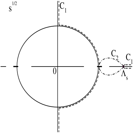
Figure 1: Singularity structure of the $\pi N\to\pi N$ amplitude (solid lines), and domains of convergence (dashed lines) characterizing the expansion (24).

In order to construct suitable conformal mappings it is necessary to discuss in some detail the analytic structure of the considered amplitudes. The singularities of the $\pi N$ scattering amplitude are given by the solid lines shown in Fig. 1 [36, 50]. Apart from the s-channel unitarity cut extending from threshold, $\sqrt{s}=m_{N}+m_{\pi}$, to infinity, there is the $u$-channel cut defined by the intervals

$$0<\sqrt{s}<m_{N}-m_{\pi}\,,\qquad m_{N}-\frac{m_{\pi}^{2}}{m_{N}}<\sqrt{s}<\sqrt{m_{N}^{2}+2\,m_{\pi}^{2}}\,,$$ (25)

the whole imaginary axis and the $t$-channel cut containing the circle $|s|=m_{N}^{2}-m_{\pi}^{2}$, and also the nucleon pole at $\sqrt{s}=\pm m_{N}$. Note that each cut has its mirror partner ($\sqrt{s}\to-\sqrt{s}$) because they originate from a Mandelstam representation written in terms of $s,t,u$.

In contrast to the $\pi N$ scattering amplitude its generalized potential is an analytic function of $\sqrt{s}$ for energies larger than the s-channel threshold. Thus it may be Taylor expanded around the point $\sqrt{s}=\mu_{E}$. However, the convergence radius would be limited by the location of the nearest branch point. The radius of convergence may be increased if some cut structures can be evaluated explicitly, such that the nearest branch point of the residual potential is more distant. For instance one may consider the u-channel cut implied by the nucleon-exchange process explicitly. As a consequence the residual potential has its nearest u-channel branch point at $\sqrt{s}=m_{N}-m_{\pi}$. Similarly the t-channel cuts close to the real line may be evaluated in $\chi$PT approximatively, it would start to build up at order $Q^{3}$. However, there is a natural limit to this construction: the u-channel and t-channel cuts turn non-perturbative at some energy necessarily.

Since we do not know a priori where the u-channel cuts turn non-perturbative we insist on that the domain $\Omega$, which we seek to specify, excludes the u-channel unitarity branch cuts, i.e.

$$(-m_{N}+m_{\pi},m_{N}-m_{\pi})\;\subset/\;\Omega\qquad\&\qquad(-i\,\infty,+i\,\infty)\;\subset/\;\Omega\,.$$ (26)

Incidentally such a construction lives in harmony with the crossing symmetry of the scattering amplitude. Given the assumption the generalized potential cannot be evaluated by means of the representation (24) for $\sqrt{s}<m_{N}-m_{\pi}$. The decomposition (24) is faithful for energies $\sqrt{s}\in\Omega$ only. Nevertheless, the full scattering amplitude can be reconstructed at $\sqrt{s}\leq m_{N}-m_{\pi}$ from the knowledge of the generalized potential at $\sqrt{s}>m_{N}+m_{\pi}$ by a crossing transformation of the solution to (8). Such a construction is consistent with crossing symmetry if the solution to (8) and its crossing transformed form coincide in the region $m_{N}-m_{\pi}<\sqrt{s}<m_{N}+m_{\pi}$. This is the case approximatively, if the matching scale $\mu_{M}$ in (8) is constructed properly. For $m_{N}-m_{\pi}<\mu_{M}<m_{N}+m_{\pi}$ the scattering amplitude remains perturbative in the matching interval, at least sufficiently close to $\sqrt{s}\sim\mu_{M}$. With our choice

$$\mu_{M}=m_{N}\,,$$ (27)

this is clearly the case (see also [22]).

Before providing a first example for a suitable conformal mapping there is yet a further issue to be discussed. Since we neglect intermediate states with mass larger than $m_{N}+2\,m_{\pi}$ one may argue to incorporate a cutoff into (8) at $\sqrt{s}\leq\Lambda_{s}\simeq m_{N}+2\,m_{\pi}$. This would induce a branch point of the generalized potential at $\sqrt{s}=\Lambda_{s}$. If we insist on the condition

$$(\Lambda_{s},\infty)\;\subset/\;\Omega\,,$$ (28)

the effect of higher mass states is part of $U_{\rm outside}(\sqrt{s}\,)$ in (24). Thus their effect renormalize the counter terms of the effective field theory, as they should. Modulo subtle effects from the chiral constraints it is impossible to discriminate the effect of a local counter term from the contribution of higher intermediate mass states in the generalized potential.

Though it is possible to use a sharp cutoff $\Lambda_{s}$ in (8) and construct conformal mappings subject to the conditions (26, 28), it is advantageous to use the limit $\Lambda_{s}\to\infty$ in (8). This avoids an artificial behavior of the scattering amplitude close to the cutoff. Rather than modifying the integral equation it suffices to adjust the generalized potential, $U(\sqrt{s}\,)$, such that the influence from the region $\sqrt{s}>\Lambda_{s}$ is irrelevant. This is readily achieved by replacing $\xi(\sqrt{s}\,)\to\xi_{\Lambda}(\sqrt{s}\,)$ in (24) with

$$\xi_{\Lambda}(\sqrt{s}\,)=\left\{\begin{array}[]{ll}\xi(\sqrt{s}\,)&{\rm for}\qquad\sqrt{s}<\Lambda_{s}\\ \xi(\Lambda_{s})&{\rm for}\qquad\sqrt{s}\geq\Lambda_{s}\ .\end{array}\right.\,,\qquad\xi^{\prime}(\Lambda_{s})=0\,.$$ (31)

where the condition $\xi^{\prime}(\Lambda_{s})=0$ guarantees a smooth behavior of $\xi_{\Lambda}(\sqrt{s}\,)$ at the cutoff scale. Though it is not immediate from the nonlinear equation (8), our claim follows from (12). For a generalized potential that is constant for $\sqrt{s}>\Lambda_{s}$, the contribution of the integral $dw$ in (12) from the region $w>\Lambda_{s}$ vanishes identically for external energies $\sqrt{s}>\Lambda_{s}$.

Consider the dashed line $C_{1}$ in Fig.  1 which encloses a domain $\Omega=\Omega_{1}$ and meets our requirements (26, 28). A conformal mapping of the domain $\Omega_{1}$ onto the unit circle is readily constructed with

$$\xi(\sqrt{s}\,)=\frac{\phi(\sqrt{s}\,)-\phi(\mu_{E})}{\phi(\sqrt{s}\,)+\phi(\mu_{E})}\,,\qquad$$

$$\phi(\sqrt{s}\,)=\frac{\sqrt{\left(s\,\Lambda_{s}^{2}-(m_{N}^{2}-m_{\pi}^{2})^{2}\right)\left(\Lambda_{s}^{2}-s\right)}}{s-m_{N}^{2}+m_{\pi}^{2}}.$$ (32)

Note that the construction of (24) does not require an explicit representation of the inverse function $\xi^{-1}(z)$. The inverse of (32) is not particularly illuminating and therefore not given here. The coefficients $U_{k}$ may be derived in application of the chain rule with

$$\frac{d}{dz}\,\xi^{-1}(z)=\left(\frac{d}{d\sqrt{s}}\,\xi(\sqrt{s}\,)\right)^{-1}\,.$$ (33)

It is not always convenient to map the unit circle onto the largest possible analyticity domain of the generalized potential, as we succeeded to do by means of (32) in the case of elastic $\pi N$ scattering. For other reactions finding such a transformation can be quite complicated.

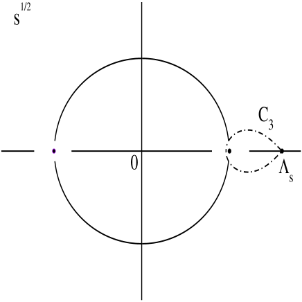
Figure 2: Singularity structure of the $\gamma N\to\pi N$ amplitude (solid lines and dots), and domains of convergence (dashed lines) characterizing the expansion (24).

The representation (24) need not converge in parts of the complex plane very distant from the physical region. Therefore it suffices to use an universal mapping for $\pi N\to\pi N$, $\gamma N\to\pi N$ and $\gamma N\to\gamma N$ reactions.

The transformation function $\xi(\sqrt{s}\,)$ is chosen to be a superposition of the function $(\Lambda_{s}-\sqrt{s}\,)^{2}$ and a Möbius transformation,

$$\xi(\sqrt{s}\,)=\frac{a_{1}\left(\Lambda_{s}-\sqrt{s}\,\right)^{2}-1}{(a_{1}-2\,a_{2})\left(\Lambda_{s}-\sqrt{s}\,\right)^{2}+1}\,,$$

$$a_{1}=\frac{1}{\left(\Lambda_{s}-\mu_{E}\right)^{2}}\,,\qquad a_{2}=\frac{1}{\left(\Lambda_{s}-\Lambda_{0}\right)^{2}}\,.$$ (34)

For $\Lambda^{2}_{0}=m_{N}^{2}-m_{\pi}^{2}$ it maps the interior of the contour $C_{2}$ in Fig. 1 onto the unit circle. Thus it meets our conditions (26-28), in particular it holds $\xi^{\prime}(\Lambda_{s})=0$. Though not necessary, it is convenient to have available the inverse mapping with

$$\xi^{-1}(x)=\Lambda_{s}-\frac{1+x}{\sqrt{(1+x)\,[(1-x)\,a_{1}+2\,a_{2}\,x]}}\,.$$ (35)

The particular form of the conformal mapping used in this work is irrelevant. We constructed various mappings that conform with the physical requirement as discussed above. Our final results show a very minor dependence on the choice thereof, that can be compensated by a slight change of free parameters.

We turn to the analytic structure of the $\gamma N\to\pi N$ amplitude [50], which is illustrated in Fig. 2. The unitarity $s$- and $u$-channel cuts are the same as in the case of $\pi N$ amplitude, except that the part of the $u$-channel cut lying on the real axis is given by

$$0<s<\frac{m_{N}}{m_{N}+m_{\pi}}\,\Big{(}m_{N}^{2}-m_{N}\,m_{\pi}-m_{\pi}^{2}\Big{)}\,.$$ (36)

The $t$-channel cut from multiple pion exchanges consists of the whole imaginary axis and two arcs defined by

$$s=\frac{2\,m_{N}^{2}+m_{\pi}^{2}-m_{t}^{2}}{2}\pm i\,\frac{\left(m_{t}^{2}-m_{\pi}^{2}\right)\sqrt{4\,m_{N}^{2}-m_{t}^{2}}}{2\,m_{t}}\,,\quad$$

$$m_{t}\in(2\,m_{\pi},2\,m_{N})\,.$$ (37)

In addition there are the $t$-channel singularities from the one-pion exchange, that includes the imaginary axis, the line $0<s<(m_{N}-m_{\pi})^{2}$ and a pole at $s=m_{N}^{2}$. We use the conformal mapping (34) with $\Lambda_{0}\simeq 901$ MeV chosen such that the contour $C_{3}$ in Fig.  2 touches the edge of the $t$-channel cut.

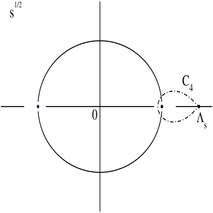
Figure 3: Singularity structure of the $\gamma N\to\gamma N$ amplitude (solid lines and dots), and domains of convergence (dashed lines) characterizing the expansion (24).

The singularity structure of the $\gamma N\to\gamma N$ amplitude is presented on Fig. 3. The unitarity $s$- and $u$-channel cuts are again the same as in the case of $\pi N$ amplitude, except that the part of the $u$-channel cut lying on the real axis is given by

$$0<s<\frac{m_{N}^{4}}{(m_{N}+m_{\pi})^{2}}\,.$$ (38)

The $t$-channel cut from the one-pion exchange consists of the whole imaginary axis and parts of the circle defined by

$$s=m_{N}^{2}-\frac{m_{t}^{2}}{2}\pm i\,\frac{m_{t}}{2}\sqrt{4\,m_{N}^{2}-m_{t}^{2}}\,,\qquad m_{t}\in(m_{\pi},2\,m_{N})\,.$$ (39)

The cut lines of a multiple $n$-pion exchange include the whole imaginary axis and a part of the arcs (39) with $m_{t}\geq n\,m_{\pi}$. We use the conformal mapping (34) with $\Lambda_{0}\simeq 877$ MeV, that maps the interior of the contour $C_{4}$ on Fig. 3 onto the unit circle. The particular value for $\Lambda_{0}$ makes the contour $C_{4}$ not to cross the part of the $t$-channel cut, corresponding to two and more-pion exchanges.

In the generalized potential based on the tree-level scattering amplitudes (2, 4, 5) only the $s$- and $u$-channel nucleon exchange and the t-channel pion-exchange contribute to $U_{\rm inside}(\sqrt{s}\,)$ in (24). The corresponding singularities must be separated in ’inside’ and ’outside’ parts as shown in Appendix B. The ’outside’ part of the potential is expanded as $U_{\rm outside}(\sqrt{s}\,)$ in (24). Given the particular choices of the conformal mappings the one-loop expressions for the three reactions contribute to $U_{\rm outside}(\sqrt{s}\,)$ only. The order to which $U_{\rm outside}(\sqrt{s}\,)$ must be expanded is discussed in the result section 3. The goal is to correlate the order of the expansion (24) with the chiral order as to obtain a generalized potential accurate in the region $\mu_{M}\sqrt{s}<\Lambda_{s}$ uniformly. Then the typical error may be identified in the chiral domain around $\sqrt{s}\simeq\mu_{M}$.

There is one peculiarity appearing when we consider the one-loop contributions to the generalized potential. We use a heavy baryon prescription for loop diagrams because it is well established for all reaction channels considered. Since the potential must possess only left-hand singularities it is necessary to subtract cut structures associated with the s-channel unitarity cut. The latter is responsible for the imaginary part of the one-loop expression at energies $\sqrt{s}>m_{\pi}+m_{N}$. In accordance with (8) we subtract from the one-loop expressions the integral

$$\sum_{c,d}\,\int_{\mu_{\rm thrs}}^{\infty}\frac{dw}{\pi}\,\frac{\sqrt{s}-\mu_{M}}{w-\mu_{M}}\,\frac{U^{(1)}_{ac}(w)\,\rho_{cd}(w)\,U^{(1)}_{db}(w)}{w-\sqrt{s}-i\epsilon}\,,$$ (40)

in a given partial wave, where $U^{(1)}(\sqrt{s})$ is the leading order tree-level potential. In (40) the reference to angular momentum and parity is omitted. The integral (40) is finite since the leading-order potential is asymptotically bounded. This is a consequence of the representation (24). The one-loop expression after subtraction of (40) still has a residual imaginary part at $\sqrt{s}>m_{\pi}+m_{N}$. It diminishes systematically if the order of the truncation in (24) and the order of chiral expansion is increased. We neglect this imaginary part as higher order and decompose the residual loop-expression according to (24). The truncation of the sum in (24) is uniform for all chiral moments of the potential, in particular for the leading-order term specifying the subtraction integral (40).

3 Numerical results

In this section we present our numerical results for the three reactions $\pi N\to\pi N$, $\gamma N\to\pi N$ and $\gamma N\to\gamma N$, where we assume the $\pi N$ channel in an s- or p-wave state. We consider the energy region from threshold up to $1.3$ GeV, which is motivated by the expected reliability of the two-channel approximation (the inelasticities in the $\pi N$ scattering are small at these energies [51, 52]). A detailed comparison with available experimental data is provided. We aim for a description of the experimental data set by solving the integral equation (8) with the generalized potential calculated in perturbation theory based on the chiral Lagrangian (1). The generalized potential is analytically continued beyond the threshold region and expanded systematically in application of suitably constructed conformal mappings as discussed in section 2.2.

3.1 $\pi N$ elastic scattering

The $\pi N$ sector is developed independently from the $\gamma N$ channel as it is treated to first order in the electric charge, $e\simeq 0.303$. The chiral Lagrangian (1) provides several free parameters. To order $Q$ the two parameters, $f$ and $g_{A}$, are relevant, where $f\simeq 92.4$ MeV is identified with the pion decay constant and $g_{A}\simeq 1.26$ with the axial-vector coupling constant of the nucleon. Owing to the Goldberger-Treiman relation $f\,g_{\pi NN}=g_{A}\,m_{N}$ one may use alternatively the empirical pion-nucleon coupling constant

$$\frac{g^{2}_{\pi NN}}{4\pi}\simeq 13.54\,,$$ (41)

as input [53]. We do not count the masses of the pion and nucleon, $m_{\pi}$ and $m_{N}$, as free parameters. They are assumed to take their empirical values properly isospin averaged. At chiral order $Q^{2}$ four additional parameters $c_{1},c_{2},c_{3},c_{4}$ arise. There remain the four counter terms proportional to $d_{1}+d_{2},d_{3},d_{5},d_{14}-d_{15}$ that turn relevant at chiral order $Q^{3}$. The parameter $d_{18}$ parameterizes the degree of violation of the Goldberger-Treiman relation. A study of pion-nucleon scattering only does not determine $g_{A}$ so that we use (41) as input. Given the empirical value for $g_{\pi NN}$ the parameter $d_{18}$ enters no longer as a free parameter in our study.

The generalized potential in (8) is decomposed into an inside and outside part based on the conformal mapping (34). While the inside part of the generalized potential is determined by the pion-nucleon coupling constant $g_{\pi NN}$, the outside part depends on the various counter terms and the order at which the expansion in (24) is truncated. As discussed in the Appendix B we perform a summation of the outside part as is implied by the contribution of the u-channel nucleon-exchange cut for $\sqrt{s}>m_{N}-m_{\pi}^{2}/m_{N}$. This controls large cancelations amongst the inside and outside parts of the potential that arise for large angular momentum. We will determine the truncation order of the residual contributions in (24) by the number of free counter terms contributing to the outside part of the potential. The original potential contains polynomial terms in $\sqrt{s}$ that are unphysical at large energies. In contrast the extrapolated potential is bounded at each order in the expansion of (24). Thus, there is an issue how many terms in the expansion should be considered. If too many terms are included the resulting potential would be unphysically large, even though the potential would be bounded asymptotically. Since the outside part of the potential is governed by left-hand cuts that are far distant, the expansion (24) should converge quickly if applied to the full potential. This is nicely confirmed by the following phenomenological study.

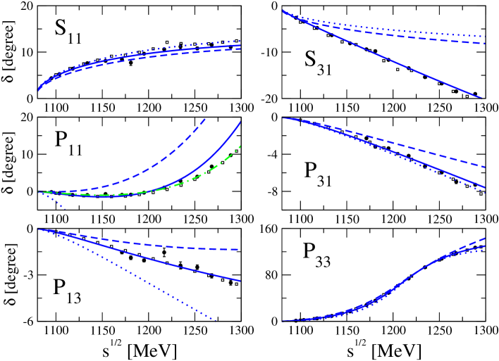
Figure 4: Results of the fit for $\pi N$ $S$ and $P$-wave phase shifts. The solid curves correspond to the full $Q^{3}$ results, the dashed curves to $Q^{2}$ results, and the dotted curves to $Q^{1}$ calculation. The dash-dotted line in the $P_{11}$ phase denote a phenomenological fit as explained it text. The data are from [51](circles) and [52](squares).

In a first step we consider the inside part of the potential as determined by the pion-nucleon coupling constant (41) but keep the values $U_{k}$ in (24) unrelated to the parameters of the chiral Lagrangian. We use $\Lambda_{s}=1500$ MeV, but checked that moderate variations with 1300 MeV $<\Lambda_{s}<$ 1600 MeV lead to almost identical results. Within this phenomenological framework we study the relevance of higher order terms in the expansion of the residual outside part of the potential. For the fits we take the energy independent phase-shift analysis [52]. The analysis from [51] is used for comparison.

The empirical partial waves $S_{11},P_{31}$ and $P_{13}$ can be well reproduced from threshold to $\sqrt{s}\leq 1300$ MeV with only the leading term in the expansion. The $S_{31}$ partial wave requires two terms. The results for these four partial waves are shown by solid curves in Fig. 4 and compared with the empirical phase shifts [51, 52].

The phase-shifts are obtained as solutions of the linear equation (12). The original non-linear equation (8) is satisfied for the $S_{11}$ and $P_{13}$ partial waves for energies from threshold to $\sqrt{s}\leq 1300$ MeV with a violation smaller than 1$\%$. The deviation is somewhat larger for the $P_{31}$ and $S_{31}$ waves, for which we obtain about 10$\%$ at the upper end. It is possible to introduce a number of CDD poles to get solutions that satisfy the causality constraint more precisely, however, this would introduce additional free parameters without clear physical meaning. The small deviations obtained we take as a signal of higher energy effects not yet controlled in the present work.

One cannot obtain a satisfactory fit for $P_{11}$ and $P_{33}$ partial waves based on the linear equation (12) without severe violation of the causality relation (8). This reflects the presence of low lying resonances in these partial waves, the $\Delta$(1232) and the N(1440) resonances. In the $P_{11}$ partial wave a numerically large contribution of the nucleon pole graph to the potential makes it impossible for the solution (8) to exist without a CDD pole. Similar findings were discussed previously in models [54, 55] also based on a single-channel approximation. After inclusion of one CDD pole, we can reproduce the $P_{33}$ partial wave with only the zeroth order coefficient in the expansion (24). The $P_{11}$ partial wave is well described in the presence of one CDD pole if the corresponding potential is expanded to first order. The results are shown in Fig. 4 by the solid line ($P_{33}$) and dash-dotted line ($P_{11}$). In both cases the set of equations (13, 15, 16) provides solutions of (8) accurate at the 1$\%$ level.

We return to our effective field theory which relates the expansion coefficients in (24) to the parameters of the chiral Lagrangian (1). At chiral order $Q^{2}$ there are four counter terms, $c_{1},..,c_{4}$ which contribute to the two s- and four p-wave potentials. There is no contribution to the potentials of higher partial waves. The coefficients $U_{k}$ in (24) posses a chiral decomposition into powers of the pion mass modulo logarithm terms. For the p-waves we have to truncate the expansion (24) at leading order, $k=0$, since any additional term may be altered arbitrarily by higher order counter terms. For the s-wave potentials the second term with, $k=1$, may be considered in addition, since the $Q^{2}$ counter terms determine the slope of the s-wave potential to leading order in a chiral expansion. However, it is unclear a priori whether one should go to the maximum order introduced above. Since the terms with $k\geq 1$ affect the high energy part of the potential we find it advantageous to consider such terms only at an order where they are determined quite precisely. To be on the safe side, we restrict ourselves to the zeroth order in the expansion (24) at chiral order $Q^{2}$. At the next order $Q^{3}$ there are additional counter terms available that lead to a precise determination of the slope of the s-wave potentials. Therefore it is justified to consider the terms with $k=1$ in (24). For the p-waves we keep the $k=0$ terms only, since the slopes of the p-wave potentials receive contributions from unknown $Q^{4}$ counter terms.

$c_{1}$ [$\rm{GeV}^{-1}$]	$c_{2}$ [$\rm{GeV}^{-1}$]	$c_{3}$ [$\rm{GeV}^{-1}$]	$c_{4}$ [$\rm{GeV}^{-1}$]
$-1.31$	$2.03$	$-5.11$	$3.59$
$\bar{d}_{1}+\bar{d}_{2}$ [$\rm{GeV}^{-2}$]	$\bar{d}_{3}$ [$\rm{GeV}^{-2}$]	$\bar{d}_{5}$ [$\rm{GeV}^{-2}$]	$\bar{d}_{14}-\bar{d}_{15}$ [$\rm{GeV}^{-2}$]
$0.13$	$0.79$	$0.68$	$-0.49$
$m_{P_{33}}$ [MeV]	$g^{\pi N}_{P_{33}}$	$m_{P_{11}}$ [MeV]	$g^{\pi N}_{P_{11}}$
$1230.7$	$11.0$	$1514$	$25$

Table 3: Parameters obtained from a fit to the empirical s- and p-wave pion-nucleon phase shifts.

We determine the chiral parameters by a fit to our phenomenological potentials, discussed above. At chiral order $Q^{3}$ it can be reproduced identically with the exception of the $P_{11}$ potential. The numerical values of our parameters are collected in Tab. 3. The solid lines in Fig. 4 show the resulting phase shifts. All phase shifts coincide with the previously discussed phenomenological phases with the exception of the $P_{11}$ phase, for which some further improvement is desirable. An accurate reproduction of the phenomenological $P_{11}$ potential would require the inclusion of the term $U_{k}$ with $k=1$ in (24). Such a term is not generated in our approach convincingly. The $P_{11}$ needs further attention, in particular the inclusion of the inelastic $\pi\pi N$ channel (see e.g. [13], [15], [56]).

The convergence properties of our approach are illustrated in Fig. 4 by additional dashed and dotted lines. The dashed lines correspond to the $Q^{2}$ calculation. It follows from the $Q^{3}$ result by switching off the contribution of the one-loop diagrams together with the parameters, $d_{1}+d_{2},d_{3},d_{5},d_{14}-d_{15}$. In addition the terms with $k=1$ in (24) are dropped. The dotted lines show the results with $c_{i}=0$, in addition, which defines the order $Q$ result. We do not change the CDD pole parameters when going from $Q^{3}$ to $Q^{2}$ or $Q^{1}$ results. The solid, dashed and dotted lines in Fig. 4 are all obtained with the same parameters as given in Tab. 3.

For all partial waves we obtain a convincing convergence pattern, although a few comments must be made. In the $P_{11}$ partial wave there is a convergence, but the $Q^{1}$ and $Q^{2}$ results are completely off the data. This is due to a significant cancelation between a large contribution from the nucleon pole term and the counter terms. The $S_{31}$ potential receives a sizeable contribution from the first order expansion term, which is absent in the $Q^{1}$ and $Q^{2}$ lines.

	current work	KA86[51]	EM98[57]
$a_{[S_{-}]}^{(\pi N)}$ [fm]	0.116	0.130	0.109 $\pm$ 0.001
$a_{[S_{+}]}^{(\pi N)}$ [fm]	0.003	-0.012	0.006 $\pm$ 0.001
$b_{[S_{-}]}^{(\pi N)}$ [$m_{\pi}^{-3}]$	0.010	0.008	0.016
$b_{[S_{+}]}^{(\pi N)}$ [$m_{\pi}^{-3}]$	-0.058	-0.044	-0.045
$a_{[P_{11}]}^{(\pi N)}$ [$m_{\pi}^{-3}$]	-0.082	-0.078	-0.078 $\pm$ 0.003
$a_{[P_{31}]}^{(\pi N)}$ [$m_{\pi}^{-3}$]	-0.048	-0.044	-0.043 $\pm$ 0.002
$a_{[P_{13}]}^{(\pi N)}$ [$m_{\pi}^{-3}$]	-0.032	-0.030	-0.033 $\pm$ 0.003
$a_{[P_{33}]}^{(\pi N)}$ [$m_{\pi}^{-3}$]	0.193	0.214	0.214 $\pm$ 0.002

Table 4: Pion-nucleon threshold parameters (see e.g. [22]).

In order to further scrutinize the consistency of our calculation we provide the threshold values of the $s$- and $p$-wave amplitudes as they come out of our calculation. In Tab. 4 they are compared with the results of different partial-wave analyses [51, 57]. Given the discrepancies among the analyses we find an acceptable overall pattern. For the p-wave scattering volumes we agree with the analysis of [51] at the $10$% level. The s-wave parameters spread most widely in the isospin even channel. A direct extraction of both scattering lengths from an analysis of pionic hydrogen and pionic deuterium data based on $\chi$PT [58] gives the following values

$$a_{[S_{-}]}^{(\pi N)}=(0.120\pm 0.003)\,{\rm fm}\,,\qquad\quad a_{[S_{+}]}^{(\pi N)}=(0.002\pm 0.003)\,{\rm fm}\,,$$ (42)

which are consistent with our results.

	$c_{1}$ [$\rm{GeV}^{-1}$]	$c_{2}$ [$\rm{GeV}^{-1}$]	$c_{3}$ [$\rm{GeV}^{-1}$]	$c_{4}$ [$\rm{GeV}^{-1}$]
current work	$-1.31$	$2.03$	$-5.11$	$3.59$
K-matrix	$-1.60$	$3.25$	$-6.34$	$3.93$
$Q^{2}$ phases [59]	$-0.57$	$2.84$	$-3.87$	$2.89$
$Q^{3}$ phases [5] fit 1	$-1.23$	$3.28$	$-5.94$	$3.47$
$Q^{3}$ phases [5] fit 2	$-1.42$	$3.13$	$-5.85$	$3.50$
$NN$ phases [60]			$-4.78$	$3.96$
	$\bar{d}_{1}+\bar{d}_{2}$ [$\rm{GeV}^{-2}$]	$\bar{d}_{3}$ [$\rm{GeV}^{-2}$]	$\bar{d}_{5}$ [$\rm{GeV}^{-2}$]	$(\bar{d}_{14}-\bar{d}_{15})$ [$\rm{GeV}^{-2}$]
current work	$0.13$	$0.79$	$+0.68$	$-0.49$
K-matrix	$3.94$	$-3.68$	$-0.17$	$-7.46$
$Q^{3}$ phases [5] fit 1	$3.06$	$-3.27$	$+0.45$	$-5.65$
$Q^{3}$ phases [5] fit 2	$3.31$	$-2.75$	$-0.48$	$-5.69$

Table 5: Comparison of low-energy constants in pion-nucleon scattering.

We continue with a discussion of our parameter set as determined from a fit to the s- and p-wave pion-nucleon phase shifts and collected in Tab. 3. The parameters related to the two CDD poles reflect the presence of the $\Delta(1232)$ in the $P_{33}$ and $N(1440)$ in the $P_{11}$ waves. They allow for an interpretation in terms of effective resonance vertices of the form

$$\mathcal{L}_{\rm eff}\,=\frac{g_{\Delta}}{f}\,\,\bar{\Delta}_{\mu}\,\vec{T}\,(\partial^{\mu}\vec{\pi})\,N\,+\frac{g_{N^{*}}}{2\,f}\,\bar{N}^{*}\,\gamma_{5}\,\gamma^{\mu}\,\big{(}\vec{\tau}\cdot(\partial_{\mu}\vec{\pi})\big{)}\,N+{\rm h.c.}\,,\qquad$$

$$g_{\Delta}=\frac{\sqrt{3}\,g^{\pi N}_{P_{33}}\,f}{m_{P_{33}}}\simeq 1.43\,,\qquad g_{N^{*}}=\frac{2\,g^{\pi N}_{P_{11}}\,f}{\sqrt{3}(m_{P_{11}}+m_{N})}\simeq 1.09\,,$$ (43)

with the isospin transition matrices normalized by $T_{i}^{\dagger}\,T_{j}=\delta_{ij}-\tau_{i}\,\tau_{j}/3$.

It is interesting to compare our parameter set with the ones from different analyses. A collection of various sets is offered in Tab. 5, where we recall central values only. We do not show statistical errors arguing that a comparison of different parameter sets is more significant in our case. At chiral order $Q^{2}$ a strict $\chi$PT fit to the $\pi N$ phase shift was performed in [59]. The sizes of the $c_{1-4}$ counter terms agrees roughly with our values, which we recall in Tab. 5 for convenience. A more quantitative agreement is expected at higher order in the chiral expansion. The parameter sets of [5] are based on a strict $\chi$PT fit at order $Q^{3}$. The empirical $\pi N$ phase shifts at energies $\sqrt{s}\leq 1100$ MeV are described. Indeed, the $c_{1-4}$ parameters agree significantly better with our set. In [5] different parameter sets are obtained, the most significant two of which are represented in Tab. 5. A further source of information on some low-energy constants is a chiral analysis of the nucleon-nucleon scattering process [60]. Here only the parameters $c_{3}$ and $c_{4}$ are relevant. The values reported in [60] differ somewhat from the results of [5]. While the value for $c_{4}$ is quite compatible with the result of [60], the value for $c_{3}$ is somewhat larger than our result.

The size of the parameter $c_{1}$ can be related to the pion-nucleon sigma term [4]. To the order $Q^{3}$ it holds

$$\sigma_{\pi N}=-4\,c_{1}\,m_{\pi}^{2}-\frac{9\,m_{\pi}^{3}}{64\,\pi\,m_{N}^{2}}\,g_{\pi NN}^{2}+{\mathcal{O}}\left(Q^{4}\right)\,,$$ (44)

which for our value of $c_{1}$ would imply $\sigma_{\pi N}=77$ MeV. This value is in contradiction to the recent determination of the sigma term based on unquenched but two-flavour QCD lattice simulations [61], which suggests a much smaller sigma term $\sigma_{\pi N}=(44-54)$ MeV. Such values appear compatible with an analysis of the subthreshold $\pi N$ amplitudes performed to chiral order $Q^{3}$ [62], which suggests a significantly smaller value for $|c_{1}|$. The scattering amplitude was reconstructed inside the Mandelstam triangle by means of dispersion relations using empirical phase shifts. This may hint at a significant sensitivity on how to determine the parameter set and reflect the influence of higher order effects. Our work does not shed additional light onto this puzzle.

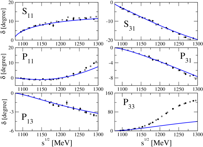
Figure 5: Results of the fit for pion-nucleon s- and p-wave phase shifts using a K-matrix ansatz. The parameters are given in Tab. 5. The data are from [51](circles) and [52](squares).

A striking discrepancy we observe for the $Q^{3}$ counter terms. For instance our value for $|\bar{d}_{3}|$ is about about four to five times as small as the values of [5, 6]. We traced the source of the discrepancy in the $Q^{3}$ counter terms as the consequence of rescattering effects. It is not related to the expansion of the potential using conformal mappings. If instead of solving the non-linear equation (8) we insist on a $K$-matrix ansatz as used in [5, 6] the parameter set is altered significantly. More specifically, in this case we apply the conformal mapping technique to the K-matrix. While the tree-level contributions to the K-matrix and the generalized potential are identical, the one-loop contributions differ. The K-matrix does not receive a contribution of the second order rescattering term (40) nor the CDD pole correction term (17). Only the real part of the one-loop diagrams contribute to the K-matrix. It is decomposed according to (24), where we use the same truncation order as in our proper approach. The result of a low-energy refit of the counter terms in the K-matrix ansatz is included in Tab. 5 by the two rows labeled ’K-matrix’. The values are much closer to the $\chi$PT fits of [5, 6]. Note that the $c_{2}$ parameter is also affected significantly by rescattering effects bringing its value close to the one obtained in [5]. The resulting $\pi$N phase shifts are shown in Fig. 5. Such an ansatz, which is at odds with the causality constraint of local quantum field theory, is nevertheless able to recover the empirical phase shifts amazingly well, with the exception of the $P_{33}$ phase. The latter is described only much below the isobar resonance.

3.2 Pion photoproduction

The generalized potential for the $\gamma N\to\pi N$ reaction is calculated to chiral order $Q^{3}$, where a multipole expansion is performed with the $\pi N$ channel in an s- or p-wave state. At leading order the potential is determined by the mass parameters and the pion-nucleon coupling constant (41). At subleading orders the anomalous magnetic moments of the proton and neutron, $\kappa_{p}$ and $\kappa_{n}$, are probed. They determine the isoscalar and isovector moments, $\kappa_{s}$ and $\kappa_{v}$, with

$$\kappa_{s}=\kappa_{p}+\kappa_{n}\,,\qquad\kappa_{v}=\kappa_{p}-\kappa_{n}\,,\qquad\kappa_{p}\simeq 1.793\,,\qquad\kappa_{n}\simeq-1.913\,,$$ (45)

where we recall also their empirical values. At order $Q^{3}$ the four counter term combinations $d_{8},d_{9},d_{20},2\,d_{21}+d_{22}$ are relevant in addition. Since we allowed for a CDD pole in the $P_{11}$ and $P_{33}$ elastic $\pi N$ amplitudes, there will be additional parameters, $g^{\gamma N}_{P_{11}}$ and $g^{\gamma N}_{1,P_{33}},g^{\gamma N}_{2,P_{33}}$, characterizing the coupling of the CDD pole to the $\gamma N$ states. An interpretation in terms of effective resonance vertices is provided by

$${\mathcal{L}}_{\rm eff}=\frac{i\,e\,f^{(1)}_{\Delta}}{2\,m_{N}}\,\bar{\Delta}^{\mu}\,\gamma_{\nu}\,\gamma_{5}\,T_{3}\,N\,F^{\mu\nu}+\frac{e\,f^{(2)}_{\Delta}}{4\,m_{N}^{2}}\,\bar{\Delta}^{\mu}\,\gamma_{5}\,T_{3}\,(\partial_{\nu}N)\,F^{\mu\nu}+\rm{h.c.}$$

$$\qquad\!-\frac{e}{4\,m_{N}}\,\bar{N}^{*}\,\sigma_{\mu\nu}\,\frac{\kappa^{N^{*}}_{s}+\kappa^{N^{*}}_{v}\,\tau_{3}}{2}\,N\,F^{\mu\nu}+\rm{h.c.}\,,$$

$$f^{(1)}_{\Delta}=\frac{m_{N}\,\sqrt{3}\,g^{\gamma N}_{1,P_{33}}(m_{N}-m_{\Delta})-2\,g^{\gamma N}_{2,P_{33}}m_{\Delta}}{e\,m_{\Delta}^{2}}\simeq 5.14\,,$$

$$f^{(2)}_{\Delta}=-\frac{4\,\sqrt{3}\,g^{\gamma N}_{1,P_{33}}\,m_{N}^{2}}{e\,m_{\Delta}^{2}}\simeq 5.89\,,$$

$$\kappa^{N^{*}}_{s}=-\frac{\sqrt{3}\,m_{N}}{e\,m_{P_{11}}}\left(g^{\gamma p}_{P_{11}}+g^{\gamma n}_{P_{11}}\right)\simeq 1.28\,,$$

$$\kappa^{N^{*}}_{v}=-\frac{\sqrt{3}\,m_{N}}{e\,m_{P_{11}}}\left(g^{\gamma p}_{P_{11}}-g^{\gamma n}_{P_{11}}\right)\simeq 1.02.$$ (46)

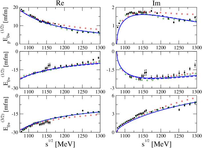
Figure 6: Electric photoproduction multipoles $E_{0+}$. The data are from [63](filled circles – energy independent analyses, open circles – energy dependent analysis) and [18](squares). The solid line denotes the $Q^{3}$ calculation, the dashed line – $Q^{2}$ calculation.

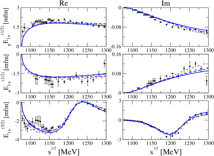
Figure 7: Electric photoproduction multipoles $E_{1+}$. The data and line conventions are as in Fig. 6.

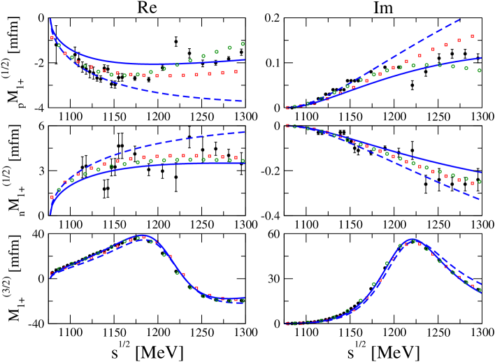
Figure 8: Magnetic photoproduction multipoles $M_{1+}$. The data and line conventions are as in Fig. 6.

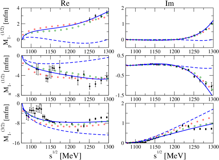
Figure 9: Magnetic photoproduction multipoles $M_{1-}$. The data and line conventions are as in Fig. 6.

The generalized potential is decomposed into an inside and outside part according to the decomposition (24). The inside part is determined unambiguously by $g_{\pi NN}$. It consists of multiple pole terms at $\sqrt{s}=m_{N}$. The outside part contains branch cuts located outside the contour $C_{3}$ of Fig. 2 only. It is expanded systematically using the conformal mapping (34) with $\Lambda_{0}=991$ MeV and $\mu_{E}=m_{N}+m_{\pi}/2$. Like for the elastic $\pi N$ potential we find it advantageous to perform a particular summation in the outside part of the photoproduction potentials. The one-pion exchange contribution provides a left-hand cut at $\sqrt{s}\leq m_{N}-m_{\pi}$ that is characterized by multiple poles at the branch point $\sqrt{s}=m_{N}-m_{\pi}$. Though such structures may be expanded systematically using (34), the convergence would be unnaturally slow in particular at large $J$. In order to treat the pole structures accurately we consider the region $m_{N}-2\,m_{\pi}\leq\sqrt{s}\leq m_{N}-m_{\pi}$ explicitly in the outside part of the potential. For more technical details we refer to Appendix B. In the residual outside part of the potential we truncate the expansion (24) at $k=0$ for the s-waves and p-waves.

$\bar{d}_{8}$ GeV2	$\bar{d}_{9}$ GeV2	$\bar{d}_{20}$ GeV2	$(2\,\bar{d}_{21}-\bar{d}_{22}$) GeV2	$g^{\gamma p}_{P_{11}}$	$g^{\gamma n}_{P_{11}}$	$g^{\gamma N}_{1,P_{33}}$	$g^{\gamma N}_{2,P_{33}}$
$3.35$	$-0.06$	$0.61$	$0.05$	$-0.33$	$0.04$	$-0.44$	$-0.93$

Table 6: Parameters obtained from photoproduction data.

The parameter set is obtained from the empirical photoproduction s- and p-wave multipoles. There are in part large discrepancies among different energy-dependent analyses [63, 18]. Therefore we try to adjust the parameters to the energy independent partial-wave analysis from [63], which is less biased than the energy dependent multipole analyses. We fit only the real part of the multipoles, since the imaginary parts are given by Watson’s theorem [64]. Our preferred parameters are given in Tab. 6.

We discuss some details of the fit procedure. We find the $\pi N$ rescattering effects important for the real parts of the s-wave multipoles. For the $p$-wave multipoles, which do not have a CDD pole contribution, rescattering effects are mostly responsible for generating the correct imaginary part, but do not modify the real parts much. The s-wave multipoles shown by solid lines in Fig. 6 depend on the particular counter term combination

$$\bar{d}_{20}+\frac{2\,\bar{d}_{21}-\bar{d}_{22}}{2}\,.$$ (47)

Since none of the other multipoles depend on $\bar{d}_{20}$, the parameter combination (47) is determined by the empirical s-wave multipoles. Given the spread in the different energy dependent analyses a satisfactory description of the s-wave multipoles is obtained.

The magnetic multipole $M_{1+}^{(3/2)}$ multipole provides a large and dominant contribution to the cross sections in the $\Delta(1232)$ resonance region [63, 18]. As a consequence the empirical error bars for this multipole are very small. The multipole depends on the particular parameter combination

$$\bar{d}_{8}+\frac{2\,\bar{d}_{21}-\bar{d}_{22}}{2}\,.$$ (48)

Since the same parameter combination enters the electric multipole $E_{1+}^{(3/2)}$ the parameter combination (48) together with the CDD pole parameters $g^{\gamma N}_{1,P_{33}},g^{\gamma N}_{2,P_{33}}$ is determined by a fit of the $E_{1+}^{(3/2)}$ and $M_{1+}^{(3/2)}$ multipoles. The solid lines in Fig. 7 and Fig. 8 show that a satisfactory description is obtained. The electric $p$-wave multipoles ${}_{p}E_{1+}^{(1/2)}$, ${}_{n}E_{1+}^{(1/2)}$, also shown in Fig. 7, do not depend on any of the parameters collected in Tab. 6. Nevertheless, the empirical multipoles are recovered reasonably by the solid lines.

There remain two parameter combinations, $\bar{d}_{9}$ and $2\,\bar{d}_{21}-\bar{d}_{22}$, that cannot be determined unambiguously from the energy independent multipole analysis [63]. Incidentally, the energy dependent analyses [63, 18] differ most significantly in those five magnetic multipoles, ${}_{p}M_{1\pm}^{(1/2)}$, ${}_{n}M_{1\pm}^{(1/2)}$ and $M_{1-}^{(3/2)}$, that are left to determine $\bar{d}_{9}$, $2\,\bar{d}_{21}-\bar{d}_{22}$ and the CDD pole parameters $g^{\gamma p}_{P_{11}}$ and $g^{\gamma n}_{P_{11}}$. In Tab. 6 we provide our preferred parameter set that took into account additional constraints from photoproduction cross sections and Compton scattering data. The five magnetic multipoles are shown in Fig. 8 and Fig. 9.

Before scrutinizing in more depth the quality of the multipole description we illustrate the convergence properties of our approach. In all Figs. 6-9 the dashed lines show the effect of switching off the contribution from the one-loop diagrams and counter terms in the photoproduction potentials. The CDD pole parameters are unchanged. For most of the multipoles this affects the results by less than $20\%$. For the $M_{1-}^{(3/2)}$ and $M_{1+}^{(1/2)}$ multipoles the difference at the highest energy considered constitute a factor of two. Also the ${}_{p}M_{1-}^{(1/2)}$ and ${}_{n}M_{1-}^{(1/2)}$ multipoles prove sensitive to the one-loop and counter term effects. This is analogous to our findings for the $P_{11}$ phase shift, the potential of which is a result of subtle cancelations. We conclude that all together there is a satisfactory convergence pattern.

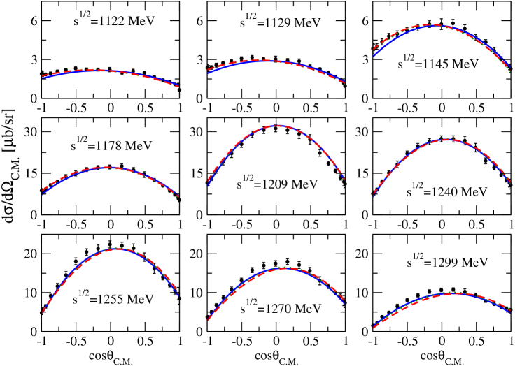
Figure 10: Differential cross section for the reaction $\gamma p\to\pi^{0}p$. The solid line corresponds to our calculation with only $s$- and $p$-wave multipoles included. The effect of higher partial waves is shown by the dashed and dotted lines as explained in the text. The data are from [65].

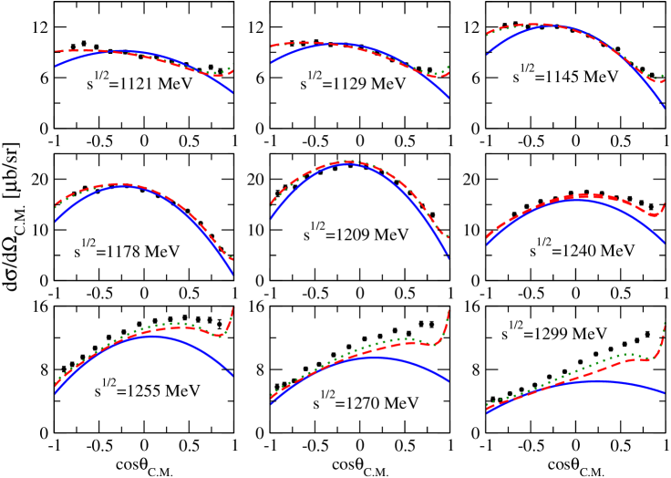
Figure 11: Differential cross section for the reaction $\gamma p\to\pi^{+}n$ with data taken from [66]. The assembly of the lines is as in Fig. 10.

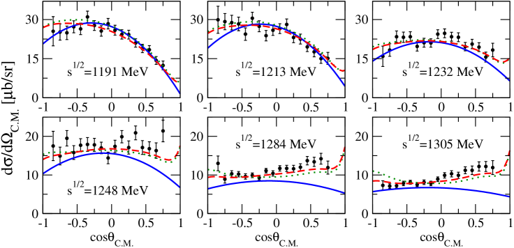
Figure 12: Differential cross section for the reaction $\gamma n\to\pi^{-}p$ with data taken from [67]. The assembly of the lines is as in Fig. 10.

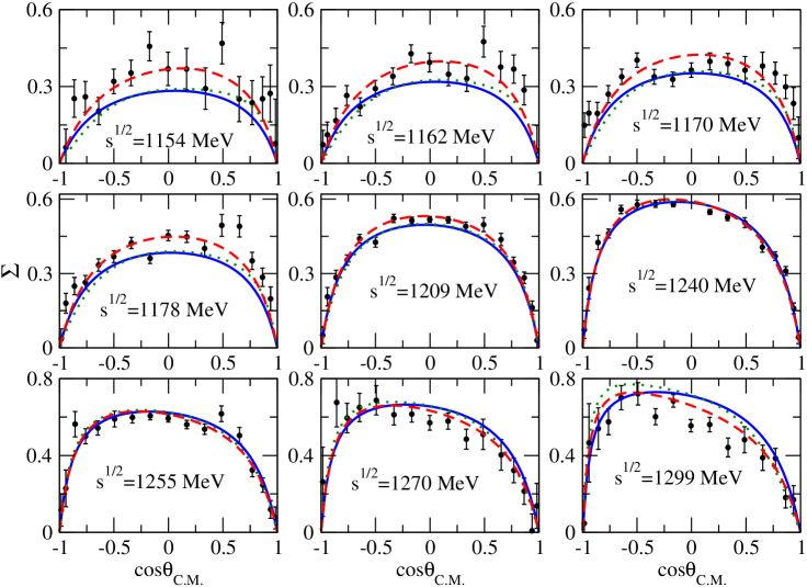
Figure 13: Beam asymmetry for the reaction $\gamma p\to\pi^{0}p$ with data taken from [65]. The assembly of the lines is as in Fig. 10.

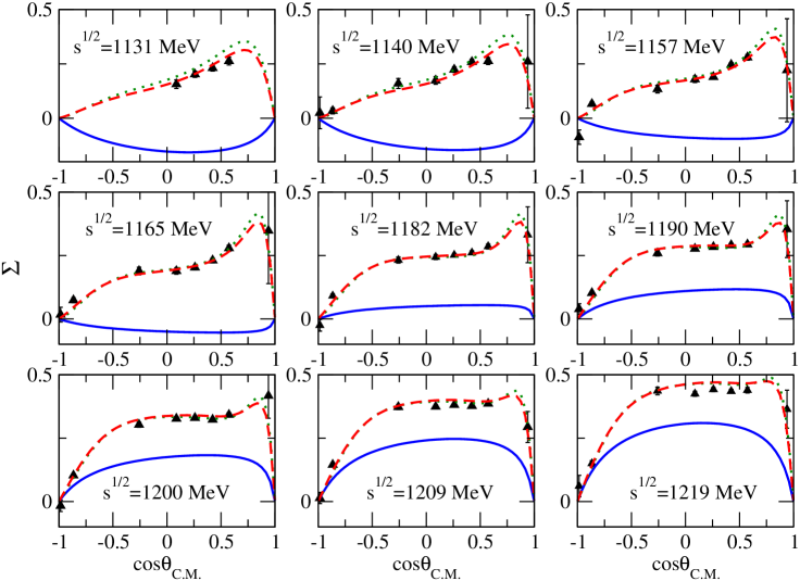
Figure 14: Beam asymmetry for the reaction $\gamma p\to\pi^{+}n$ with data taken from [68]. The assembly of the lines is as in Fig. 10.

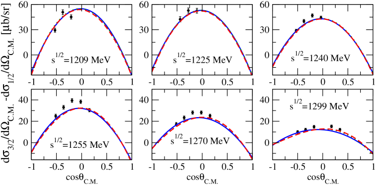
Figure 15: Helicity asymmetry for the reaction $\gamma p\to\pi^{0}p$ with data taken from [66]. The assembly of the lines is as in Fig. 10.

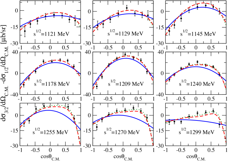
Figure 16: Helicity asymmetry for the reaction $\gamma p\to\pi^{+}n$ with data taken from [66]. The assembly of the lines is as in Fig. 10.

We proceed with a more direct comparison of our results with empirical cross section data. This is achieved by taking our s- and p-wave multipoles in the calculation of differential and polarization cross sections. Higher partial waves are supplemented from two different sources. First we compute the higher multipoles within our given scheme but neglect the final state interaction, i.e. we identify the generalized potential with the partial-wave production amplitude. Note that the one-loop contribution of a strict $\chi$PT computation does not contribute to any of the higher partial waves for which we neglect the final state interaction. Second we take the higher multipoles from the energy dependent analysis [18]. In Figs. 10-11 we present differential cross section data from several recent and precise measurements [65, 67, 66, 68] for the $\gamma p\to\pi^{0}p$ and $\gamma p\to\pi^{+}n$ and $\gamma n\to\pi^{-}p$ reactions. Fig. 10 illustrates that our multipoles describe the differential cross section for the $\pi^{0}$ production off the proton accurately, the effect of higher multipoles being quite small. Recall the absence of the $t$-channel pion exchange process in this reaction. After adding the effects of the higher multipoles the same is true for the $\pi^{\pm}$ production cross sections of Fig. 12 and Fig. 11. The solid lines show the contributions from the s- and p-wave multipoles. The dashed and dotted lines result upon adding up the higher multipoles from our theory and [18] respectively. The effect of using different higher multipoles, dashed versus dotted line, is irrelevant for our conclusions.

We compute the beam and helicity asymmetries of the two reactions $\gamma p\to\pi^{0}p$ and $\gamma p\to\pi^{+}\,n$, for which empirical data exist. Their relation to the multipole amplitudes is given in Appendix A.3. The results are shown in Figs. 13-16. After inclusion of higher partial wave contributions all considered observables are nicely reproduced in the whole energy region considered. Higher partial wave contributions are significant in the production of charged pions.

Like for $\pi N$ elastic scattering we scrutinize the near-threshold physics for pion photoproduction in some detail. We compute the s- and p-wave threshold production parameters. Empirically it is well established that in neutral pion photoproduction there is a strong cusp effect at the $\pi^{+}\,n$ threshold [69, 70]. To obtain accurate results we depart from the isospin formulation and perform a coupled-channel computation in the particle basis using physical masses for the nucleons and pions. Isospin breaking effects are not considered for the generalized potential being estimated to be of minor importance. No additional parameters arise.

In Tab. 7 we present the s-wave threshold parameters for neutral and charged pion production. Our results are compared to the empirical values, which we reproduce quite accurately. Tab. 7 recalls also the results of a $\chi$PT analysis accurate to chiral order $Q^{4}$. While $\chi$PT appears well converging for charged pion production a less convincing convergence pattern is found for the neutral pion production [8]. The order $Q^{3}$ value obtained in [8] for the $E_{0^{+}}$ threshold amplitude is $+0.90\cdot 10^{-3}/m_{\pi^{+}}$, in striking conflict with experiment. Only the inclusion of the order $Q^{4}$ terms lead to a value compatible with the empirical data. A precise prediction of the threshold amplitude is difficult in $\chi$PT since it depends sensitively on $Q^{4}$ counter terms that are not well known. The threshold value given in [71] is based on an analysis of the latest MAMI data set [70]. It is amusing to observe that we obtain accurate threshold parameters already based on the chiral Lagrangian truncated at order $Q^{3}$. We reiterate that our threshold values are a consequence of a parameter fit to the production data at energies excluding the threshold region.

			Present work	$\chi$PT ($Q^{4}$)	Experiment
$E_{0+}$	($\pi^{+}n$)	[$10^{-3}/m_{\pi^{+}}$]	$\phantom{-}27.4$	$\phantom{-}28.2$ [9]	$28.06\pm 0.27\pm 0.45$ [72]
$E_{0+}$	($\pi^{-}p$)	[$10^{-3}/m_{\pi^{+}}$]	$-31.5$	$-32.7$ [9]	$-31.5\pm 0.8$ [73]
$E_{0+}$	($\pi^{0}\,p$)	[$10^{-3}/m_{\pi^{+}}$]	$-1.12$	$-1.16$ [74]	$\begin{array}[]{ll}-1.32\pm 0.05\pm 0.06\,\text{\cite[cite]{[\@@bibref{}{Bergstrom:1996fq}{}{}]}}\\ -1.23\pm 0.08\pm 0.03\,\text{\cite[cite]{[\@@bibref{}{Schmidt:2001vg}{}{}]}}\end{array}$

Table 7: Threshold values for the $E_{0^{+}}$ multipole in the $\gamma\,p\to\pi^{0}\,p$, $\gamma\,n\to\pi^{-}\,n$ and $\gamma\,p\to\pi^{0}\,p$ reactions.

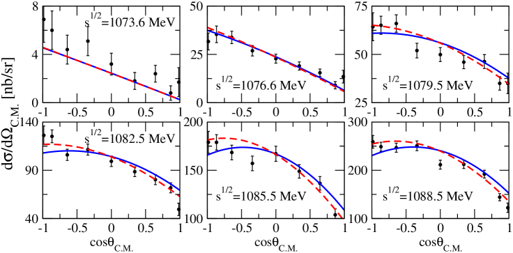
Figure 17: Near threshold differential cross section for the reaction $\gamma p\to\pi^{0}p$ with data taken from [75, 70]. Shown are results from our coupled-channel theory including isospin breaking effects as are implied by the use of empirical pion and nucleon masses. The solid lines correspond to our calculation with only $s$- and $p$-wave multipoles included. The effect of higher partial waves is shown by the dashed lines.

Further significant information on the near-threshold region of neutral pion photoproduction is available. The s-wave amplitude shows a strong energy dependence with a prominent cusp structure at the $\pi^{+}\,n$ threshold [70]. Since the threshold region shows an intriguing interplay of the s- and p-wave multipoles we confront our theory in Fig. 17 with empirical differential cross section of the Mainz group directly. Given the fact that we did not fit the parameters to those data an excellent description is achieved.

			Present work	$\chi$PT ($Q^{3}$)	Experiment
$\bar{P}_{1}$	($\pi^{0}\,p$)	[$10^{-3}/m_{\pi^{+}}^{2}$]	$10.2$	$9.4$ [74]	$9.46\pm 0.05\pm 0.28$ [70]
$\bar{P}_{2}$	($\pi^{0}\,p$)	[$10^{-3}/m_{\pi^{+}}^{2}$]	$-10.7$	$-10.0$ [74]	$-9.5\pm 0.09\pm 0.28$ [70]
$\bar{P}_{3}$	($\pi^{0}\,p$)	[$10^{-3}/m_{\pi^{+}}^{2}$]	$10.3$	$10.6$ [74]	$11.32\pm 0.11\pm 0.34$ [70]

Table 8: Threshold values of p-wave multipoles in neutral pion photoproduction.

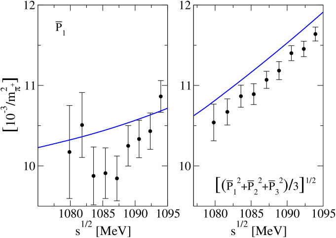
Figure 18: Energy dependence of the p-wave amplitude $\bar{P}_{1}$ (l.h.p.) and $(\bar{P}_{1}^{2}+\bar{P}_{2}^{2}+\bar{P}_{3}^{2})^{1/2}/\sqrt{3}$ (r.h.p.) in neutral pion photoproduction. The data are from [76]. The solid lines follow from the coupled-channel theory.

From the near-threshold differential cross section two combinations of p-wave threshold parameters may be extracted. It is customary to introduce the following three combinations of p-wave multipole amplitudes,

$$\bar{p}_{\rm cm}\,\bar{P}_{1}=3\,E_{1+}+M_{1+}-M_{1-}\,,\qquad\bar{p}_{\rm cm}\,\bar{P}_{2}=3\,E_{1+}-M_{1+}+M_{1-}\,,$$

$$\bar{p}_{\rm cm}\,\bar{P}_{3}=2\,M_{1+}+M_{1-}\,,$$ (49)

which all vanish at the production threshold with $\bar{p}_{\rm cm}=0$. A complete determination of all three p-wave threshold amplitudes requires additional information. For this purpose a measurement of the near-threshold photon asymmetry suffices [70].

At leading orders in a chiral expansion $\bar{P}_{1}$ and $\bar{P}_{2}$ do not depend on any of the $Q^{3}$ counter terms. The threshold behavior of $\bar{P}_{1}$ and $\bar{P}_{2}$ is predicted in terms of the electromagnetic charge, the pion-nucleon coupling constant and the masses of the pions and nucleons only [8, 74, 71]. In Tab. 8 we recall their numerical values from [74]. The chiral corrections of order $Q^{4}$ were studied in [71] and shown to be subject to sizeable cancelation effects amongst chiral loops and further counter terms dominated by isobar exchange processes. In contrast $\bar{P}_{3}$ receives a contribution from the $Q^{3}$ counter term combination $\bar{d}_{8}+\bar{d}_{9}$ and there is no parameter-free prediction accurate to order $Q^{3}$.

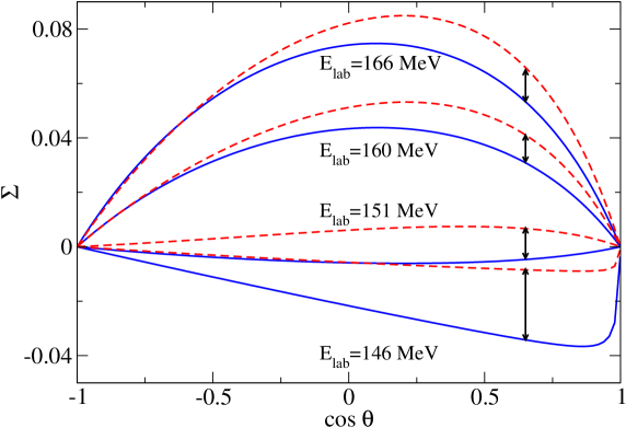
Figure 19: Energy dependence of the photon asymmetry in neutral pion photoproduction from the coupled-channel theory. The solid lines correspond to our calculation with only $s$- and $p$-wave multipoles included. The effect of higher partial waves is shown by the dashed lines.

In Tab. 8 we confront our p-wave threshold parameters with those of [70, 74]. Though we are in qualitative agreement with the empirical values obtained by the Mainz group there is a significant discrepancy. Contrasting conclusions were drawn from the $\chi$PT computation to order $Q^{4}$ in [71], which was able to accommodate the threshold values presented in [70]. It is interesting to locate the source of the observed discrepancies. For this purpose we provide a comparison with near-threshold data of the Saskatoon group [76]. In Fig. 18 the empirical energy dependence of $\bar{P}_{1}$ is shown against our theoretical result. Given the energy dependence of our theory one would expect a threshold value of around $10$, a value close to our result. This is striking disagreement with the value of $9.3\pm 0.09$ extracted in [76], based on a different assumption on the energy dependence. In Fig. 18 we present also the empirical constraint on the mean p-wave amplitudes. We find an excellent description of the energy dependence where the overall magnitude is overestimated by less than 2$\%$.

We finally turn to the near-threshold photon asymmetry measurement of the Mainz group [70]. A direct comparison is not straightforward since an average from threshold to 166 MeV laboratory photon energies was performed. In Fig. 19 we show the result of our computation at four different energies demonstrating a sign change in the asymmetry at energies below the mean value of 159.5 MeV in the Mainz experiment. At the mean energy our photon asymmetry is about a factor four to five smaller than the averaged value presented in [70]. Within our scheme we have no freedom to significantly increase that value without destroying the successful description of the photoproduction multipoles at higher energies. It is interesting to recall that a negative photon asymmetry was obtained also in [77, 78] based on a dispersion-relation analysis of photo production data. Given such a sign change an average over the photon energy depends on the very details of the averaging procedure.

A significant effect of higher partial wave contributions on the asymmetry is illustrated by the dashed lines in Fig. 19. The possible importance of d-wave amplitudes in the photon asymmetry was pointed out in [79] recently.

Since the near-threshold behavior of the photon asymmetry is subject to subtle cancelation effects it would be important to extend our analysis to order $Q^{4}$ and see whether the observed sign change persists. Also further data taking on the photon asymmetry like planned and ongoing at Mainz [80, 81] is highly welcome.

3.3 Proton Compton scattering

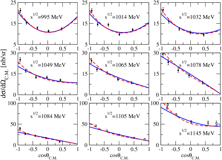
Figure 20: Differential cross section for Compton scattering off the proton as a function of the center-of-mass scattering angle. The data are from [82]($\bullet$) and [83] ($\square$). The solid lines follow from the our partial-wave amplitudes with $J\leq 3/2$. The dashed lines show the effect of partial-wave contributions with $J>3/2$ as explained in the text.

We turn to Compton scattering off the proton. Since counter terms start to contribute at the order $Q^{4}$ there are no additional free parameters to be determined in our work. The CDD pole parameters are set already from pion-nucleon scattering and pion photoproduction. In the following we present parameter free results based on a generalized potential accurate to order $Q^{3}$.

Since we neglect the intermediate $\gamma N$ states the Compton amplitude reduces to the sum of two contributions. There is a direct term and a rescattering term, which depends quadratically on the photoproduction amplitude. The latter has already been calculated and presented in the previous section. In the rescattering part we consider $\pi N$ states in s- or p-waves only. Higher partial-waves cannot be treated here because those were neither considered in elastic pion-nucleon scattering nor in pion photoproduction. We argue that this suffices for calculating cross sections in the energy region considered. Higher partial waves are largely suppressed by the $\pi N$ phase space proportional to $p_{\rm cm}^{2\,L+1}$ entering the integral in (8). On the other hand for the direct contribution we take into account all $J=\frac{1}{2}$ and $J=\frac{3}{2}$ waves. The positive and negative parity partial-wave amplitudes are of equal importance as a consequence of gauge invariance. We checked that these waves reproduce the Born diagrams quite accurately up to energies of about 1300 MeV. According to our strategy we have to apply an analytic extrapolation to the generalized Compton potential. Using the conformal mapping as detailed in section 2.2 we truncate this expansion at zeroth order. Terms beyond the zeroth order cannot be justified since $Q^{4}$ counter terms may alter those significantly.

Our results for the differential cross section and beam asymmetry are presented in Figs. 20-22 against empirical data. We find agreement with the data taking into account some discrepancy of the different data sets. The photon threshold region, the pionproduction threshold region, and the isobar region are equally well reproduced. This is nicely illustrated by Fig. 23, which shows the energy dependence of the cross section at fixed scattering angle $\theta\simeq 90^{\circ}$. There seems to be a systematic undershooting of the backward differential cross section for energies $\sqrt{s}<1150$ MeV. We believe, that a natural explanation for this effect are missing higher order contributions. Indeed adding to the $J\leq 3/2$ result contribution from additional partial-wave with $J>3/2$ as implied by the direct term in our scheme the differential cross section is increased towards the data in backward direction. This is shown by the dashed lines in Figs. 20-22.

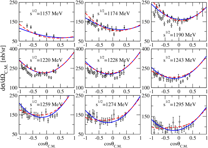
Figure 21: Differential cross section for Compton scattering off the proton as a function of the center-of-mass scattering angle. The data are from [83] ($\square$),[68]($\blacktriangle$), [84]($\circ$) and the lines are as in Fig. 20.

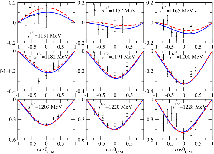
Figure 22: Beam asymmetry for Compton scattering off the proton as a function of the center-of-mass scattering angle. The data are from [68] and the lines are as in Fig. 20.

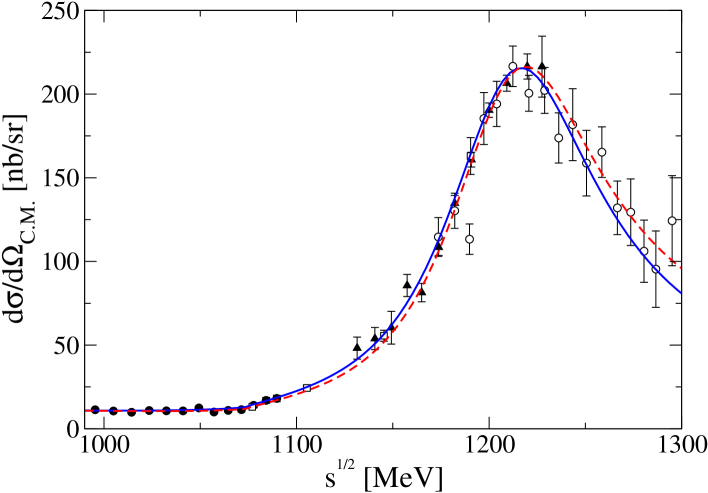
Figure 23: Compton scattering off the proton as a function of energy at scattering angle $\theta=90^{\circ}$. The data are from [82]($\bullet$), [83] ($\square$),[68]($\blacktriangle$), [84]($\circ$) and the lines are as in Fig. 20. The experimental values correspond to scattering angles closest to $\theta=90^{\circ}$ taken in the interval $86^{\circ}<\theta<94^{\circ}$.

The low-energy physics of Compton scattering is characterized by various nucleon polarizabilities. For a definition of the polarizabilities see e.g. [85]. It is instructive to express the latter in terms of partial-wave amplitudes $T^{J}_{\pm,ab}(\sqrt{s}\,)$ as constructed in Appendix A.4 and used in (8). In our case the indices $a$ and $b$ run form one to two, reflecting the two polarizations of the photon. The electric and magnetic dipole polarizabilities $\alpha_{p}$ and $\beta_{p}$ probe partial-wave amplitudes with $J=\frac{1}{2}$ and $J=\frac{3}{2}$ at threshold, where there are constraints set by crossing symmetry. To be specific the following identity holds

$$\Delta T^{\,\gamma p\to\gamma p,\frac{3}{2}}_{\pm,22}(\sqrt{s}=m_{p})=\frac{3}{4}\,\Delta T^{\,\gamma p\to\gamma p,\frac{1}{2}}_{\mp,11}(\sqrt{s}=m_{p})\,,$$ (50)

which can be derived from the expressions given in Appendix A.4 and [86]. In (50) the ’$\Delta$’ indicates the need to subtract the contributions from the nucleon exchange processes. In our approach the crossing relation (50) is obeyed strictly. This is a consequence of the matching scale $\mu_{M}$ in (8) being identified with the nucleon mass. In turn we recover the one-loop $\chi$PT results of [1]:

$$\alpha_{p}=\frac{3}{16\,\pi\,m_{p}^{3}}\,\Delta T^{\,\gamma p\to\gamma p,\frac{1}{2}}_{+,11}(m_{p})=\frac{5\,e^{2}\,g_{\pi NN}^{2}}{384\,\pi^{2}\,m_{N}^{2}\,m_{\pi}}\simeq 13.0\cdot 10^{-4}\,\rm{fm}^{3}\,,$$

$$\beta_{p}=\frac{3}{16\,\pi\,m_{p}^{3}}\,\Delta T^{\,\gamma p\to\gamma p,\frac{1}{2}}_{-,11}(m_{p})=\frac{e^{2}\,g_{\pi NN}^{2}}{768\,\pi^{2}\,m_{N}^{2}\,m_{\pi}}\simeq\phantom{x}1.3\cdot 10^{-4}\,\rm{fm}^{3}\,,$$ (51)

which are known to agree well with the experimental values $\alpha_{p}=(12.0\pm 0.6)\cdot 10^{-4}\,\rm{fm}^{3}$, $\beta_{p}=(1.9\pm 0.6)\cdot 10^{-4}\,\rm{fm}^{3}$ [87] (for a recent development see [88]). Further polarizabilities probe derivatives of partial-wave amplitudes at threshold. Since we expand the generalized potential to the zeroth order in the conformal mapping only, we can extract reliably only electric and magnetic dipole polarizabilities.

4 Summary

We presented a uniform description of photon- and pion-nucleon scattering data up to and beyond the isobar region. The results are based on partial-wave amplitudes derived from the chiral Lagrangian formulated with photon, pion and nucleon fields. Electromagnetic gauge invariance is kept rigourously.

Our study is based on partial-wave amplitudes that have the MacDowell relations and that are free of kinematical constraints. In the presence of spin the derivation of such amplitudes is tedious and presented in this work for pion photoproduction and Compton scattering for the first time. The partial-wave scattering amplitudes were decomposed into parts with left- and right-hand cuts only. Such a separation is electromagnetic-gauge invariant. The part with left-hand cuts only defines a generalized potential, which is evaluated relying on the chiral Lagrangian truncated at order $Q^{3}$. The part with right-hand cuts only is derived as a solution of a non-linear integral equation. The latter combines the constraints set by causality and coupled-channel unitary in a systematic fashion. The reparametrization invariance of local quantum field theory is obeyed strictly.

The non-linear integral equation does not permit solutions always. The unitarity constraint implies an asymptotic bound on the generalized potential, which is at odds with any polynomial energy dependence as generated by $\chi$PT. This problem was resolved by performing an analytic continuation constrained by the known asymptotic bound. The generalized potential was evaluated in a strict chiral expansion to order $Q^{3}$. It followed an analytic extrapolation in terms of suitably constructed conformal mappings. The non-linear integral equations were solved by N/D techniques, where the presence of two CDD poles in the N/D ansatz reflect the physics of the isobar and Roper resonances. It was demonstrated that the presence of a CDD pole corresponds to an infinite set of local counter terms in the chiral Lagrangian.

Even though the parameter set was adjusted to the scattering data avoiding the near threshold region, we obtained results that are compatible with the empirical threshold behavior nevertheless. The accurate pion-nucleon scattering lengths as measured in pionic-hydrogen and deuterium systems are recovered. In order to compare with the near threshold data available for neutral pion photoproduction we considered isospin breaking effects as implied by the empirical pion and nucleon masses. Despite the fact that we reproduce the differential cross section accurately we predict s- and p-wave threshold parameters that differ somewhat from the values obtained by the Mainz and Saskatoon groups. We traced this discrepancy to an additional energy dependence in the p-wave multipoles that was not considered in the threshold analyses of the two groups. As a striking prediction we find a sign change in the photon asymmetry at photon energies below 160 MeV. Further data on the photon asymmetry, that do not average over a large threshold region, would be highly welcome. Our threshold analysis was completed by a determination of the electric and magnetic dipole polarizabilties, for which their empirical values are reproduced accurately.

A detailed comparison of threshold parameters with results from $\chi$PT was given. In contrast to a strict $\chi$PT computation that requires in many cases important contributions from the $Q^{4}$ terms, we obtained an accurate description of threshold observable based on the chiral Lagrangian truncated at order $Q^{3}$. The apparent slow convergence of $\chi$PT in particular for the neutral pion photoproduction process is overcome largely by our resummation approach that protects causality and unitarity rigourously. A more convincing convergence pattern is found in our scheme.

While in our work we focused on s- and p-waves we provided a comprehensive comparison with scattering data up to energies of $\sqrt{s}\sim 1300$ MeV. In case of pion-nucleon scattering this was achieved by a comparison with the phase shifts, which are sufficiently well known from various partial-wave analyses and were reproduced quite accurately. In contrast the electric and magnetic multipole amplitudes of the pion photoproduction process suffer still from ambiguities. A comparison with recent analyses of the MAID and SAID groups was offered in this case. Since we observe in part significant discrepancies amongst the two groups and our results we provided complementary results for differential cross section, beam and helicity asymmetry. We focused on the processes which were measured most accurately. For neutral pion photo production the influence of additional partial waves was shown to be of minor importance. For charged pion photo production the role of higher partial wave contributions builds up significantly. A comparison with a representative selection of high-quality data is offered by combining our results for the s- and p-wave multipoles with the higher partial-waves from our theory where we neglected the final state interaction. This way an accurate description of the data was achieved. The empirical data on Compton scattering off the proton were reproduced with the $J=\frac{1}{2}$ and $J=\frac{3}{2}$ partial-waves. The influence of higher partial wave contributions was shown to be of minor importance. Differential cross sections and beam asymmetries were reproduced equally well from threshold to the isobar region.

Appendix A Partial-wave amplitudes and kinematic constraints

Throughout this appendix we adopt the notation $w_{\mu}=p_{\mu}+q_{\mu}=\bar{p}_{\mu}+\bar{q}_{\mu}$, where $p_{\mu}$ and $\bar{p}_{\mu}$ are the initial and final nucleon $4$-momenta respectively, whereas $q_{\mu}$ and $\bar{q}_{\mu}$ are the $4$-momenta of initial pion (photon) and final pion (photon) respectively. The Madelstam variables are $s=w^{2}$, $t=(\bar{q}-q)^{2}=(\bar{p}-p)^{2}$ and $u=(\bar{q}-p)^{2}=(\bar{p}-q)^{2}$. In the center of mass frame the energies of the nucleons are denoted by $E$, $\bar{E}$, and the energies of initial pion (photon) and final pion (photon) by $\omega$, $\bar{\omega}$. For the initial state it holds

$$E=\Bigg{\{}\begin{array}[]{ll}\frac{s+m_{N}^{2}-m_{\pi}^{2}}{2\,\sqrt{s}}&{\rm for}\;\;\pi N\\ \frac{s+m_{N}^{2}}{2\,\sqrt{s}}&{\rm for}\;\;\gamma N\end{array}\,,\qquad\quad\omega=\Bigg{\{}\begin{array}[]{ll}\frac{s-m_{N}^{2}+m_{\pi}^{2}}{2\,\sqrt{s}}&{\rm for}\;\;\pi N\\ \frac{s-m_{N}^{2}}{2\,\sqrt{s}}&{\rm for}\;\;\gamma N\end{array}\,,$$ (56)

$$E^{2}=m_{N}^{2}+p_{\rm cm}^{2}\,,\qquad\quad\omega^{2}=\Bigg{\{}\begin{array}[]{ll}m_{\pi}^{2}+p_{\rm cm}^{2}&{\rm for}\;\;\pi N\\ p_{\rm cm}^{2}&{\rm for}\;\;\gamma N\end{array}\,,$$ (59)

with the relative momentum $p_{\rm cm}$ of the center of mass frame. Analogous expressions hold for the final state. The center-of-mass scattering angle $\theta$ is introduced with

$$p^{\mu}=(E,0,0,-p_{\rm cm})\,,\qquad\bar{p}^{\mu}=(\bar{E},-\bar{p}_{\rm cm}\,\sin\theta,0,-\bar{p}_{\rm cm}\,\cos\theta)\,.$$ (60)

A.1 Isospin decomposition

We recall the isospin decomposition for the $\pi N$ elastic amplitude and the one for the photoproduction of the pion (see e.g. [90]). The elastic amplitude $T^{ab}$ and the production amplitude $T^{a}$ may be decomposed as follows

$$T_{\pi N\to\pi N}^{ab}=T^{(+)}_{\pi N}\,\delta^{ab}+T^{(-)}_{\pi N}\,i\,\varepsilon^{abc}\,\tau_{c}=\Big{(}\frac{1}{3}\,\tau_{a}\,\tau_{b}\Big{)}\,T^{(\frac{1}{2})}_{\pi N}+\Big{(}\delta_{ab}-\frac{1}{3}\,\tau_{a}\,\tau_{b}\Big{)}T^{(\frac{3}{2})}_{\pi N}\,,$$

$$T_{\gamma N\to\pi N}^{a}=T^{(-)}_{\gamma N}\,i\,\varepsilon^{a3c}\,\tau_{c}+T^{(0)}_{\gamma N}\,\tau^{a}+T^{(+)}_{\gamma N}\,\delta^{a3}=\sqrt{\frac{3}{2}}\,\Big{(}\delta_{a3}-\frac{1}{3}\,\tau_{a}\,\tau_{3}\Big{)}\,T^{(\frac{3}{2})}_{\gamma N}$$

$$\qquad\quad\;\;\,+\,\sqrt{\frac{1}{3}}\,\tau_{a}\,\Big{(}\frac{1+\tau_{3}}{2}\,T^{(\frac{1}{2})}_{\gamma p}+\frac{1-\tau_{3}}{2}\,T^{(\frac{1}{2})}_{\gamma n}\Big{)}\,,$$ (61)

where $a$ and $b$ are the isospin indices of the final and initial pions respectively. The elastic amplitudes $T^{(I)}_{\pi N}$ with isospin $I=\frac{1}{2}$ and $I=\frac{3}{2}$ are linear combinations of $T^{(\pm)}_{\pi N}$. The production amplitudes $T^{(I)}_{\gamma N}$ with isospin $I=\frac{1}{2},\frac{3}{2}$ and $N=p,n$ are related to $T^{(0,\pm)}_{\gamma N}$. It holds

$$T_{\gamma p}^{(\frac{1}{2})}=\sqrt{3}\,T^{(0)}_{\gamma N}+\frac{1}{\sqrt{3}}\,T^{(+)}_{\gamma N}+\frac{2}{\sqrt{3}}\,T^{(-)}_{\gamma N}\,,\qquad T^{(\frac{1}{2})}_{\pi N}=T^{(+)}_{\pi N}+2\,T^{(-)}_{\pi N}\,,$$

$$T_{\gamma n}^{(\frac{1}{2})}=\sqrt{3}\,T^{(0)}-\frac{1}{\sqrt{3}}\,T^{(+)}_{\gamma N}-\frac{2}{\sqrt{3}}\,T^{(-)}_{\gamma N}\,,$$

$$T^{(\frac{3}{2})}_{\gamma p}=T^{(\frac{3}{2})}_{\gamma n}=\sqrt{\frac{2}{3}}\,\Big{(}T^{(+)}_{\gamma N}-T^{(-)}_{\gamma N}\Big{)}\,,\qquad\quad\;\;\,T^{(\frac{3}{2})}_{\pi N}=T^{(+)}_{\pi N}-T^{(-)}_{\pi N}\,,$$ (62)

where the amplitudes are introduced with respect to normalized states. This is convenient in a coupled-channel framework. The isospin amplitudes of (62) are related to the ones in the particle basis as follows

$$T_{\,\pi^{0}\,p\to\,\pi^{0}\,p} = \frac{1}{3}\,T^{(\frac{1}{2})}_{\pi N}+\frac{2}{3}\,T^{(\frac{3}{2})}_{\pi N}=T_{\pi^{0}\,n\to\pi^{0}\,n}\,,$$

$$T_{\pi^{+}n\to\pi^{+}n} = \frac{2}{3}\,T^{(\frac{1}{2})}_{\pi N}+\frac{1}{3}\,T^{(\frac{3}{2})}_{\pi N}=T_{\pi^{-}p\to\pi^{-}p}\,,$$

$$T_{\pi^{0}\,p\to\pi^{+}n} = \frac{\sqrt{2}}{3}\left(T^{(\frac{1}{2})}_{\pi N}-T^{(\frac{3}{2})}_{\pi N}\right)=-T_{\pi^{0}n\to\pi^{-}p}\,,$$ (63)

and

$$T_{\gamma p\to\pi^{0}\,p} = \sqrt{\frac{1}{3}}\,T_{\gamma p}^{(\frac{1}{2})}+\sqrt{\frac{2}{3}}\,T_{\gamma p}^{(\frac{3}{2})}\,,\qquad T_{\gamma n\to\pi^{0}n}=-\sqrt{\frac{1}{3}}\,T_{\gamma n}^{(\frac{1}{2})}+\sqrt{\frac{2}{3}}\,T_{\gamma n}^{(\frac{3}{2})}\,,$$

$$T_{\gamma p\to\pi^{+}n} = \sqrt{\frac{2}{3}}\,T_{\gamma p}^{(\frac{1}{2})}-\sqrt{\frac{1}{3}}\,T_{\gamma p}^{(\frac{3}{2})}\,,\qquad T_{\gamma n\to\pi^{-}p}=\sqrt{\frac{2}{3}}\,T_{\gamma n}^{(\frac{1}{2})}+\sqrt{\frac{1}{3}}\,T_{\gamma n}^{(\frac{3}{2})}\,.$$ (64)

A.2 $\pi N$ elastic scattering

The on-shell pion-nucleon scattering amplitude may be decomposed into invariant amplitudes

$$T(\bar{q},q;w)=F_{1}(s,t)+F_{2}(s,t)\,w/$$

$$\qquad\quad\;\;\;\;\,=F_{+}(\sqrt{s},t)\,\Bigg{\{}\frac{1}{2}\,+\frac{w/}{2\sqrt{w^{2}}}\Bigg{\}}+F_{-}(\sqrt{s},t)\,\Bigg{\{}\frac{1}{2}\,-\frac{w/}{2\sqrt{w^{2}}}\Bigg{\}}\,,$$ (65)

where we suppress the reference to the isospin channel and the on-shell nucleon Dirac-spinors. The two sets of amplitudes introduced in (65) are related to each other through

$$F_{\pm}=F_{1}\pm F_{2}\,\sqrt{s}\,.$$ (66)

Since the amplitudes $F_{1}$, $F_{2}$ are free of kinematic singularities, so are the amplitudes $F_{\pm}$ except for the relation

$$F_{-}(+\sqrt{s},t)=F_{+}(-\sqrt{s},t)\,.$$ (67)

One may adopt the viewpoint that there is in fact only a single invariant amplitude $F_{+}(\sqrt{s},t)$ which characterizes the scattering amplitude fully. The latter amplitude is free of any kinematic constraints.

The partial-wave amplitudes with definite parity, $P$, and total angular momentum, $J$, are most economically given in terms of the $F_{\pm}$ amplitudes. We recall from [91, 22]

$$t_{\pm}^{J}(\sqrt{s}\,)=\pm\,\frac{E\pm m_{N}}{2\,m_{N}}\left(p_{\rm cm}^{2}\right)^{J-\frac{1}{2}}\int_{-1}^{1}\frac{d\cos\theta}{2}\,\Bigg{\{}\frac{P_{J-\frac{1}{2}}(\cos\theta)}{\left(p_{\rm cm}^{2}\right)^{J-\frac{1}{2}}}\,F_{\pm}(\sqrt{s},t)$$

$$\qquad\qquad-\,\frac{P_{J+\frac{1}{2}}(\cos\theta)}{\left(p_{\rm cm}^{2}\right)^{J+\frac{1}{2}}}\,(E\mp m_{N})^{2}\,F_{\mp}(\sqrt{s},t)\Bigg{\}}\,,$$ (68)

where $\pm$ characterizes the helicity of the nucleon. The parity of the amplitude $t_{\pm}^{J}(\sqrt{s}\,)$ is given by $P=\pm$ for $J-\frac{1}{2}$ odd and $P=\mp$ for $J-\frac{1}{2}$ even.

The expressions (68) imply the standard normalization of the helicity amplitudes $t_{\pm}^{J}(\sqrt{s}\,)$. We introduce partial-wave amplitudes $T_{\pm}^{J}(\sqrt{s}\,)$, that enjoy the MacDowell relation

$$T_{-}^{J}(+\sqrt{s}\,)=T_{+}^{J}(-\sqrt{s}\,)\,,$$ (69)

and that are free of kinematic singularities and zeros, where we admit constraints at $s=0$ as the only exception. From (68) it follows that the helicity amplitudes $t_{\pm}^{J}(\sqrt{s}\,)$ suffer from kinematic zeros at threshold and pseudo-threshold defined by the conditions

$$E\pm m_{N}=\frac{s+m_{N}^{2}-m_{\pi}^{2}}{2\,\sqrt{s}}\pm m_{N}=0\,.$$ (70)

This conclusion is possible only since the invariant functions $F_{\pm}(\sqrt{s},\,t)$ are kinematicly unconstrained. With

$$T_{\pm}^{J}(\sqrt{s}\,)=\frac{2\,m_{N}\sqrt{s}}{E\pm m_{N}}\left(\frac{\sqrt{s}}{p_{\rm cm}}\right)^{2\,J-1}\,t_{\pm}^{J}(\sqrt{s}\,)\,,\quad$$ (71)

we recover the covariant partial-wave amplitudes derived previously in [22] up to a factor $s^{J}$. That factor $s^{J}$ is introduced in the present work as to render the phase-space density

$$\rho_{\pm}^{J}(\sqrt{s}\,)=-\Im{\,\frac{1}{T_{\pm}^{J}(\sqrt{s}\,)}}=\frac{p_{\rm cm}\,(E\pm m_{N})}{8\,\pi\,s}\left(\frac{p_{\rm cm}^{2}}{s}\right)^{J-1/2}\,,$$ (72)

constant at asymptotically large $\sqrt{s}$.

We turn to the technical details of the effective field theory. The tree-level diagrams (2) implied by the Lagrangian density (1) lead to the invariant amplitudes

$$F^{(I)}_{\pm}(\sqrt{s},t)=\Big{\{}\frac{1}{2\,f^{2}}\,(\pm\sqrt{s}-m_{N})+\frac{c_{4}}{f^{2}}\,(\bar{q}\cdot q-(\pm\sqrt{s}-m_{N})^{2})$$

$$\quad+\,\frac{d_{3}}{2\,f^{2}\,m_{N}^{3}}\,(s-m_{N}^{2}-m_{\pi}^{2})\,(s-m_{N}^{2}-\bar{q}\cdot q)\,(s-m_{N}^{2}+m_{\pi}^{2}-2\,\bar{q}\cdot q)$$

$$\quad+\,\Big{[}2\,\frac{d_{1}+d_{2}}{f^{2}\,m_{N}}\,(\bar{q}\cdot q)+4\,\frac{d_{5}}{f^{2}\,m_{N}}\,m_{\pi}^{2}\,\Big{]}\,(s-m_{N}^{2}-\bar{q}\cdot q)\Big{\}}\,C_{-}^{(I)}$$

$$+\,\Big{\{}-4\,\frac{c_{1}}{f^{2}}\,m_{\pi}^{2}+\frac{c_{2}}{2\,f^{2}\,m_{N}^{2}}(s-m_{N}^{2}-m_{\pi}^{2})\,(s-m_{N}^{2}+m_{\pi}^{2}-2\,\bar{q}\cdot q)$$

$$\quad+\,2\,\frac{c_{3}}{f^{2}}\,(\bar{q}\cdot q)+\frac{d_{14}-d_{15}}{f^{2}\,m_{N}}\,(s-m_{N}^{2}-\bar{q}\cdot q)\,(\bar{q}\cdot q-(\pm\sqrt{s}-m_{N})^{2})\Big{\}}\,C_{+}^{(I)}$$

$$-\,\frac{(g_{A}-2\,m_{\pi}^{2}\,d_{18})^{2}}{4\,f^{2}}\frac{(\pm\sqrt{s}-m_{N})^{2}}{m_{N}\pm\sqrt{s}}\,C_{s,N}^{(I)}$$

$$+\,\frac{(g_{A}-2\,m_{\pi}^{2}\,d_{18})^{2}}{4\,f^{2}}\Big{(}\frac{4\,m_{N}^{2}(\pm\sqrt{s}-m_{N})}{u-m_{N}^{2}}+m_{N}\pm\sqrt{s}\Big{)}\,C_{u,N}^{(I)}\,,$$ (73)

where the isospin coefficients $C^{(I)}_{...}$ are detailed in Tab. 1. The amplitudes (73) receive contributions from different orders in a strict chiral expansion. While the counter terms $c_{...}$ start to contribute at order $Q^{2}$, the counter terms $d_{...}$ contribute at $Q^{3}$.

At chiral order $Q^{3}$ one needs to consider a set of ultraviolet divergent one-loop diagrams. The counter term combinations $d_{1}+d_{2}$, $d_{3}$, $d_{5}$ and $d_{14}-d_{15}$ are required for their renormalization. In the heavy-baryon chiral perturbation theory the corresponding loop diagrams were computed in [5]. The results were expressed in terms of the frame-dependent amplitudes, $g$ and $h$, that arise naturally in the center-of-mass frame with two-component nucleon spinors,

$$T_{\rm cm}=\frac{E+m_{N}}{2\,m_{N}}\,\Big{\{}g+i\,\vec{\sigma}\cdot(\vec{q}_{\pi,\rm{out}}\times\vec{q}_{\pi,\rm{in}})\,h\,\Big{\}}\,.$$ (74)

with the Pauli matrices $\sigma_{i}$. The invariant amplitudes $F_{\pm}$ of (65) follow with

$$F_{+}=g-h\,p_{\rm cm}^{2}\,\cos\theta\,,\qquad\quad F_{-}=-h\,(E+m_{N})^{2}\,.$$ (75)

We recall from [5] the explicit result

$$g^{(I)} = \Big{\{}i\,\frac{\omega^{2}}{8\pi f^{4}}\,p_{\rm cm}+\frac{g_{A}^{2}}{32\pi\,f^{4}}\,(m_{\pi}^{2}-2\,t)\,\Big{[}m_{\pi}+\frac{2\,m_{\pi}^{2}-t}{2\,\sqrt{-t}}\arctan{\frac{\sqrt{-t}}{2\,m_{\pi}}}\Big{]}$$

$$\quad+\,\frac{g_{A}^{4}}{24\pi\,f^{4}\,\omega^{2}}\,\big{(}t-2\,m_{\pi}^{2}+2\,\omega^{2}\big{)}\big{(}i\,p_{\rm cm}^{3}-m_{\pi}^{3}\big{)}\Big{\}}\,C^{(I)}_{+}\,,$$

$$+ \Big{\{}\frac{2\,\omega}{f^{2}}(2\,m_{\pi}^{2}-t)(\bar{d}_{1}+\bar{d}_{2})+\frac{4\,\omega^{3}}{f^{2}}\,\bar{d}_{3}+\frac{8\,\omega\,m_{\pi}^{2}}{f^{2}}\,\bar{d}_{5}$$

$$\quad+\,\frac{1}{32\pi^{2}\,f^{4}}\,\Big{[}\frac{\omega}{3}\,(4\,m_{\pi}^{2}-t)\sqrt{1-\frac{4\,m_{\pi}^{2}}{t}}\log\frac{\sqrt{4\,m_{\pi}^{2}-t}+\sqrt{-t}}{2\,m_{\pi}}$$

$$\quad-\,4\,\omega^{2}\,p_{\rm cm}\Big{(}\log{\frac{\omega+p_{\rm cm}}{m_{\pi}}}-i\,\frac{\pi}{2}\Big{)}+\frac{\omega}{9}\left(18\,\omega^{2}-12\,m_{\pi}^{2}+\frac{5}{2}\,t\right)\Big{]}$$

$$\quad-\,\frac{g_{A}^{2}}{24\pi^{2}f^{4}}\,\Big{[}\frac{1}{4}\,\omega\,(5\,t-8\,m_{\pi}^{2})\,\sqrt{1-\frac{4\,m_{\pi}^{2}}{t}}\,\log\frac{\sqrt{4\,m_{\pi}^{2}-t}+\sqrt{-t}}{2\,m_{\pi}}$$

$$\quad+\,2\,\omega\,m_{\pi}^{2}-\frac{13}{24}\,\omega\,t\Big{]}+\frac{g_{A}^{4}}{96\pi^{2}\,f^{4}\,\omega^{2}}\,\Big{[}2\,p_{\rm cm}^{3}\Big{(}\log{\frac{\omega+p_{\rm cm}}{m_{\pi}}}-i\,\frac{\pi}{2}\Big{)}$$

$$\quad+\,2\,m_{\pi}^{2}\,\omega-\frac{5}{3}\,\omega^{3}\Big{]}\,(2\,m_{\pi}^{2}-2\,\omega^{2}-t)\Big{\}}\,C^{(I)}_{-}\,,$$

$$h^{(I)} = \Big{\{}\frac{2\,\omega}{f^{2}}\,(\bar{d}_{14}-\bar{d}_{15})$$ (76)

$$\quad-\,\frac{g_{A}^{4}}{24\pi^{2}\,f^{4}\,\omega^{2}}\,\Big{[}m_{\pi}^{2}\,\omega+\frac{\omega^{3}}{6}+p_{\rm cm}^{3}\,\Big{(}\log{\frac{\omega+p_{\rm cm}}{m_{\pi}}}-i\frac{\pi}{2}\Big{)}\Big{]}\Big{\}}\,C_{+}^{(I)}\,,$$

$$+ \Big{\{}\frac{g_{A}^{2}}{32\pi\,f^{4}}\,\Big{[}\frac{t-4\,m_{\pi}^{2}}{2\,\sqrt{-t}}\arctan{\frac{\sqrt{-t}}{2\,m_{\pi}}}-m_{\pi}\Big{]}$$

$$\quad+\,\frac{g_{A}^{4}}{24\,\pi\,f^{4}\,\omega^{2}}\left(i\,p_{\rm cm}^{3}-m_{\pi}^{3}\right)\Big{\}}\,C_{-}^{(I)}\,,$$

where the $\bar{d}$’s are the scale independent renormalized coupling constants according to [5].

At order $Q^{3}$ it is legitimate to add up the loop contribution (76) to the tree-level contribution (73) via the relation (75) provided the substitution rules

$$\frac{g_{A}-2\,m_{\pi}^{2}\,d_{18}}{f}\to\frac{g_{\pi NN}}{m_{N}}\,,\qquad d_{i}\to 0\,,$$ (77)

are used in (73). In the one-loop result (76) we replace $g_{A}\to f\,g_{\pi NN}/m_{N}$ for convenience. The loop contributions are specified in a manner such that it is justified to use the empirical pion-decay constant with $f=f_{\pi}$ in the tree-level expressions (73).

A.3 Pion photoproduction amplitudes

We decompose the on-shell pion photoproduction amplitude into four invariant amplitudes, where we will suppress reference to the channel specifics (see (61)). There are different choices possible. Chew et al. constructed in [90] the CGLN amplitudes, $A(s,t),B(s,t),C(s,t)$ and $D(s,t)$ that are free of kinematic constraints [38, 92]. Since we are interested in a partial-wave decomposition of the invariant amplitudes it is advantageous to use a different set showing the MacDowell symmetry [36] in addition. Like for elastic pion-nucleon scattering it is possible to introduce invariant amplitudes $F_{1}^{\pm}(\sqrt{s},t)$ and $F_{2}^{\pm}(\sqrt{s},t)$ with

$$F^{-}_{i}(+\sqrt{s},t)=F^{+}_{i}(-\sqrt{s},t)\,,$$ (78)

that are free of kinematic constraints. We recall the definition of the CGLN amplitudes and relate them to the $F_{1-2}^{\pm}(\sqrt{s},t)$ amplitudes

$$i\,T_{\mu}(\bar{q},q;w)=\gamma_{5}\,\gamma_{\mu}\,q/\,A(s,t)-2\,\gamma_{5}\,\big{[}\left(\bar{q}\cdot q\right)P_{\mu}-\left(P\cdot q\right)\bar{q}_{\mu}\big{]}\,B(s,t)$$

$$\qquad+\,\gamma_{5}\,\big{[}\left(\bar{q}\cdot q\right)\gamma_{\mu}-q/\,\bar{q}_{\mu}\big{]}\,C(s,t)$$

$$\qquad+\,2\,\gamma_{5}\,\big{[}\left(P\cdot q\right)\gamma_{\mu}-q/\,P_{\mu}-m_{N}\,\gamma_{\mu}\,q/\big{]}\,D(s,t)$$

$$\qquad=\sum_{i=1}^{2}\,\Big{\{}F^{+}_{i}(\sqrt{s}\,,\,t)\,L^{(i,+)}_{\mu}(\bar{q},q,w)+F^{-}_{i}(\sqrt{s}\,,\,t)\,L^{(i,-)}_{\mu}(\bar{q},q,w)\Big{\}}\,,$$

$$L^{(1,\pm)}_{\mu}(\bar{q},q,w)=\gamma_{5}\,\Big{(}\frac{1}{2}\pm\frac{w/}{2\,\sqrt{s}}\Big{)}\,\gamma_{\mu}\,q/\,,\qquad$$

$$L^{(2,\pm)}_{\mu}(\bar{q},q,w)=\gamma_{5}\,\Big{(}\frac{1}{2}\pm\frac{w/}{2\,\sqrt{s}}\Big{)}\,\Big{(}(\bar{q}\cdot q)\,\gamma_{\mu}-q/\,\bar{q}_{\mu}\Big{)}\,,$$ (79)

where $P_{\mu}=(p_{\mu}+\bar{p}_{\mu})/2$. The two representations in (79) are equivalent in the presence of an on-shell initial nucleon spinor, $p^{2}=m_{N}^{2}$ and

$$F^{\pm}_{1} = A-B\,(\bar{q}\cdot q)-D\left(m_{N}\pm\sqrt{s}\,\right),$$

$$F^{\pm}_{2} = C-D-B\left(m_{N}\pm\sqrt{s}\,\right).$$ (80)

¿From (80) it follows our claim that the amplitudes $F^{\pm}_{1}(\sqrt{s}\,,\,t)$, and $F^{\pm}_{2}(\sqrt{s}\,,\,t)$ are free of kinematic constraints but (78).

The partial-wave amplitudes with definite parity, $P$, and total angular momentum, $J$, corresponding to anti-aligned and aligned helicities of the initial nucleon and photon are readily expressed in terms of the invariant amplitudes $F^{\pm}_{1,2}$ introduced in (79). We derive

$$t^{J}_{\pm,1}(\sqrt{s}\,)=\frac{(\bar{p}_{\rm cm}\,p_{\rm cm})^{J-\frac{1}{2}}}{\sqrt{2\,m_{N}\,\sqrt{s}}}\sqrt{\frac{\bar{E}\pm m_{N}}{2\,m_{N}}}\int_{-1}^{1}\,\frac{d\cos\theta}{2}\,\Bigg{\{}\Big{[}\mp 2\,\omega\,\sqrt{s}\,F^{\pm}_{1}(\sqrt{s},t)$$

$$\qquad+\big{(}(\sqrt{s}\mp m_{N})\,\bar{\omega}\,\omega\pm m_{N}\,\bar{p}_{\rm cm}\,p_{\rm cm}\,\cos\theta\big{)}\,F^{\pm}_{2}(\sqrt{s},t)$$

$$\qquad+\,\omega\,\sqrt{s}\,(\bar{E}\pm m_{N})\,F^{\mp}_{2}(\sqrt{s},t)\Big{]}\,\omega\,(\bar{E}\mp m_{N})\,\frac{P_{J+\frac{1}{2}}(\cos\theta)}{(\bar{p}_{\rm cm}\,p_{\rm cm})^{J+\frac{1}{2}}}$$

$$\quad\pm\,\Big{[}-\omega\,\sqrt{s}\,\big{(}2\,F_{1}^{\mp}(\sqrt{s},t)\pm(\bar{E}\mp m_{N})\,F_{2}^{\pm}(\sqrt{s},t)\big{)}$$

$$\qquad+\,\Big{(}m_{N}\,\bar{p}_{\rm cm}\,p_{\rm cm}\,\cos\theta\mp(\sqrt{s}\pm m_{N})\,\bar{\omega}\,\omega\Big{)}\,F^{\mp}_{2}(\sqrt{s},t)\Big{]}\,\frac{P_{J-\frac{1}{2}}(\cos\theta)}{(\bar{p}_{\rm cm}\,p_{\rm cm})^{J-\frac{1}{2}}}\,\Bigg{\}}\,,$$

$$t^{J}_{\pm,2}(\sqrt{s}\,)=(\bar{p}_{\rm cm}\,p_{\rm cm})^{J-\frac{1}{2}}\sqrt{\frac{\sqrt{s}}{2\,m_{N}}}\sqrt{\frac{\bar{E}\pm\bar{m}_{N}}{2\,m_{N}}}\int_{-1}^{1}\frac{d\cos\theta}{2}\,\Bigg{\{}$$

$$\quad\mp\,\Big{[}{\textstyle{\sqrt{\frac{2\,J+3}{2\,J-1}}}}\,\omega\,(\bar{E}\pm m_{N})\,F^{\mp}_{2}(\sqrt{s},t)$$

$$\qquad+\,{\textstyle{\sqrt{\frac{2\,J-1}{2\,J+3}}}}\,\bar{p}_{\rm cm}\,p_{\rm cm}\,\cos\theta\,F^{\pm}_{2}(\sqrt{s},t)\Big{]}\,\omega\,(\bar{E}\mp m_{N})\,\frac{P_{J+\frac{1}{2}}(\cos\theta)}{(\bar{p}_{\rm cm}\,p_{\rm cm})^{J+\frac{1}{2}}}$$

$$\quad\pm\,\Big{[}{\textstyle{\sqrt{\frac{2\,J+3}{2\,J-1}}}}\,\bar{p}_{\rm cm}\,p_{\rm cm}\,\cos\theta\,F^{\mp}_{2}(\sqrt{s},t)$$

$$\qquad+\,{\textstyle{\sqrt{\frac{2\,J-1}{2\,J+3}}}}\,(\bar{E}\mp m_{N})\,\omega\,F^{\pm}_{2}(\sqrt{s},t)\Big{]}\,\frac{P_{J-\frac{1}{2}}(\cos\theta)}{(\bar{p}_{\rm cm}\,p_{\rm cm})^{J-\frac{1}{2}}}\Bigg{\}}\,,$$ (81)

except for $J=\frac{1}{2}$ with $t^{\frac{1}{2}}_{\pm,2}=0$. The parity of the amplitudes $t_{\pm,1}^{J}(\sqrt{s}\,)$ and $t_{\pm,2}^{J}(\sqrt{s}\,)$ is given by $P=\pm$ for $J-\frac{1}{2}$ odd and $P=\mp$ for $J-\frac{1}{2}$ even. The electric and magnetic multipoles [90, 93] can be expressed in terms of helicity partial-wave amplitudes $t^{IJ}_{\pm,1}(\sqrt{s}\,)$ and $t^{IJ}_{\pm,2}(\sqrt{s}\,)$ as follows

$$E^{(I)}_{(J-\frac{1}{2})+}=\frac{m_{N}}{4\,\pi\,\sqrt{s}}\,\frac{-\sqrt{2}}{2\,J+1}\left(t^{IJ}_{+,1}-\sqrt{\frac{2\,J-1}{2\,J+3}}\,t^{IJ}_{+,2}\right)\left\{\begin{array}[]{lll}\sqrt{\frac{1}{3}}&\quad{\rm for}&\quad I=\frac{1}{2}\\ \sqrt{\frac{3}{2}}&\quad{\rm for}&\quad I=\frac{3}{2}\\ \end{array}\right.,$$ (84)

$$M^{(I)}_{(J-\frac{1}{2})+}=\frac{m_{N}}{4\,\pi\,\sqrt{s}}\,\frac{-\sqrt{2}}{2\,J+1}\left(t^{IJ}_{+,1}+\sqrt{\frac{2\,J+3}{2\,J-1}}\,t^{IJ}_{+,2}\right)\left\{\begin{array}[]{lll}\sqrt{\frac{1}{3}}&\quad{\rm for}&\quad I=\frac{1}{2}\\ \sqrt{\frac{3}{2}}&\quad{\rm for}&\quad I=\frac{3}{2}\\ \end{array}\right.,$$ (87)

(88)

$$E^{(I)}_{(J+\frac{1}{2})-}=\frac{m_{N}}{4\,\pi\,\sqrt{s}}\,\frac{+\sqrt{2}}{2\,J+1}\left(t^{IJ}_{-,1}+\sqrt{\frac{2\,J+3}{2\,J-1}}\,t^{IJ}_{-,2}\right)\left\{\begin{array}[]{lll}\sqrt{\frac{1}{3}}&\quad{\rm for}&\quad I=\frac{1}{2}\\ \sqrt{\frac{3}{2}}&\quad{\rm for}&\quad I=\frac{3}{2}\\ \end{array}\right.\,,$$ (91)

$$M^{(I)}_{(J+\frac{1}{2})-}=\frac{m_{N}}{4\,\pi\,\sqrt{s}}\,\frac{-\sqrt{2}}{2\,J+1}\left(t^{IJ}_{-,1}-\sqrt{\frac{2\,J-1}{2\,J+3}}\,t^{IJ}_{-,2}\right)\left\{\begin{array}[]{lll}\sqrt{\frac{1}{3}}&\quad{\rm for}&\quad I=\frac{1}{2}\\ \sqrt{\frac{3}{2}}&\quad{\rm for}&\quad I=\frac{3}{2}\\ \end{array}\right.\,,$$ (94)

where we made explicit the isospin structure. Note that the conventional electric and magnetic multipole amplitudes are introduced with respect to isospin states that are not normalized. Since the partial-wave helicity amplitudes are defined with respect to normalized states the factors $\sqrt{\frac{1}{3}}$ and $\sqrt{\frac{3}{2}}$ arise.

The differential cross section, $d\sigma/d\Omega$, the beam asymmetry, $\Sigma$, and the helicity asymmetry, $d\,(\sigma_{3/2}-\sigma_{1/2})/d\Omega$, are expressed conveniently in terms of helicity matrix elements (see e.g. [94]). It holds

$$\frac{d\sigma}{d\Omega}=\frac{\bar{p}_{\rm cm}}{2\,p_{\rm cm}}\left(|H_{N}|^{2}+|H_{SA}|^{2}+|H_{SP}|^{2}+|H_{D}|^{2}\right)\,,$$

$$\Sigma\,\frac{d\sigma}{d\Omega}=\frac{\bar{p}_{\rm cm}}{p_{\rm cm}}\,\Re\left(H_{SP}H_{SA}^{*}-H_{N}H_{D}^{*}\right)\,,$$

$$\frac{d\sigma_{3/2}}{d\Omega}-\frac{d\sigma_{1/2}}{d\Omega}=\frac{\bar{p}_{\rm cm}}{p_{\rm cm}}\left(|H_{SP}|^{2}+|H_{D}|^{2}-|H_{N}|^{2}-|H_{SA}|^{2}\right)\,,$$ (95)

with $x=\cos\theta$ and

$$H_{N\;\;}=\frac{m_{N}}{4\pi\,\sqrt{s}}\,\cos\frac{\theta}{2}\,\sum_{J}\left(t^{J}_{+,1}-t^{J}_{-,1}\right)\left(P^{\prime}_{J+\frac{1}{2}}(x)-P^{\prime}_{J-\frac{1}{2}}(x)\right)\,,$$

$$H_{SA}=-\frac{m_{N}}{4\pi\,\sqrt{s}}\,\sin\frac{\theta}{2}\,\sum_{J}\left(t^{J}_{+,1}+t^{J}_{-,1}\right)\left(P^{\prime}_{J+\frac{1}{2}}(x)+P^{\prime}_{J-\frac{1}{2}}(x)\right)\,,$$

$$H_{SP}=\frac{m_{N}}{4\pi\,\sqrt{s}}\,\frac{-\sin\theta\cos{\frac{\theta}{2}}}{\sqrt{(J-\frac{1}{2})(J+\frac{3}{2})}}\,\sum_{J}\left(t^{J}_{+,2}-t^{J}_{-,2}\right)\left(P^{\prime\prime}_{J+\frac{1}{2}}(x)-P^{\prime\prime}_{J-\frac{1}{2}}(x)\right)\,,$$

$$H_{D\;\;}=\frac{m_{N}}{4\pi\,\sqrt{s}}\,\frac{\sin\theta\sin{\frac{\theta}{2}}}{\sqrt{(J-\frac{1}{2})(J+\frac{3}{2})}}\,\sum_{J}\left(t^{J}_{+,2}+t^{J}_{-,2}\right)\left(P^{\prime\prime}_{J+\frac{1}{2}}(x)+P^{\prime\prime}_{J-\frac{1}{2}}(x)\right)\,.$$

We construct partial-wave amplitudes, $T^{J}_{\pm,1}(\sqrt{s}\,)$ and $T^{J}_{\pm,2}(\sqrt{s}\,)$, that are free of kinematic constraints. According to (81) the helicity partial-wave amplitudes have zeros at thresholds and pseudothresholds

$$\bar{E}\pm m_{N}=\frac{s+m_{N}^{2}-m_{\pi}^{2}}{2\,\sqrt{s}}\pm m_{N}=0\,.$$ (96)

Taking into account (59) and

$$\bar{p}_{\rm cm}\,p_{\rm cm}\,\cos\theta=\frac{t}{2}+\bar{E}\,E-m_{N}^{2}\,,$$ (97)

it is readily seen that the two amplitudes

$$\sqrt{2\,m_{N}\,\sqrt{s}}\,\sqrt{\frac{2\,m_{N}}{\bar{E}\pm m_{N}}}\,\frac{t^{J}_{\pm,1}(\sqrt{s}\,)}{(\bar{p}_{\rm cm}\,p_{\rm cm})^{J-\frac{1}{2}}}\,,$$

$$\sqrt{\frac{m_{N}}{2\,\sqrt{s}}}\,\sqrt{\frac{2\,m_{N}}{\bar{E}\pm m_{N}}}\,\frac{t^{J}_{\pm,2}(\sqrt{s}\,)}{(\bar{p}_{\rm cm}\,p_{\rm cm})^{J-\frac{1}{2}}}\,,$$ (98)

are free of kinematic constraints but one exception. From (81) it follows that the amplitudes $t^{J}_{\pm,1}(\sqrt{s}\,)$ and $t^{J}_{\pm,2}(\sqrt{s}\,)$ are linear dependent at $\omega=p_{\rm cm}=0$ even after pulling out the common phase-space factor. In that limit the two partial-wave amplitudes are characterized by the terms proportional to $\bar{p}_{\rm cm}\,p_{\rm cm}\,\cos\theta\,F_{2}^{\mp}(\sqrt{s},t)$ in (81). It follows

$$\frac{t^{J}_{\pm,1}(\sqrt{s}\,)-\frac{m_{N}}{\sqrt{s}}\,\sqrt{\frac{2\,J-1}{2\,J+3}}\,t^{J}_{\pm,2}(\sqrt{s}\,)}{(\bar{p}_{\rm cm}\,p_{\rm cm})^{J-\frac{1}{2}}}\stackrel{{\scriptstyle p_{\rm cm}\to 0}}{{=}}O(p_{\rm cm})\,.$$ (99)

Owing to (99) it is straightforward to derive the following set of partial-wave amplitudes

$$T^{J}_{\pm,a}(\sqrt{s}\,) = \sqrt{\frac{4\,m_{N}^{2}\,\sqrt{s}}{\bar{E}\pm m_{N}}}\left(\frac{s}{\bar{p}_{\rm cm}\,p_{\rm cm}}\right)^{J-\frac{1}{2}}\!t^{J}_{\pm,b}(\sqrt{s}\,)\left(\begin{matrix}\frac{\sqrt{s}}{p_{\rm cm}}&0\\ -\sqrt{\frac{2\,J-1}{2\,J+3}}\,\frac{m_{N}}{p_{\rm cm}}&1\end{matrix}\right)_{ba}\!,$$ (100)

which are free of any constraints. As in the case of $\pi N$ scattering the factor of $s^{J}$ was chosen so that the $\gamma N$ phase-space density is asymptotically constant (see (9)). The MacDowell relations

$$T_{-,1}^{J}(+\sqrt{s}\,)=-T_{+,1}^{J}(-\sqrt{s}\,)\,,\qquad T_{-,2}^{J}(+\sqrt{s}\,)=+T_{+,2}^{J}(-\sqrt{s}\,)$$ (101)

hold.

We turn to the details of the effective field theory. The Lagrangian density (1) leads with (4, 79) to the tree-level expressions

$$F_{1}^{\pm} = -\frac{e\,(g_{A}-2\,m_{\pi}^{2}\,d_{18})\,(m_{N}\pm\sqrt{s}\,)}{4\,f\,m_{N}\,(m_{N}\mp\sqrt{s}\,)}\,\tilde{C}_{s,N}$$

$$- \frac{e\,(g_{A}-2\,m_{\pi}^{2}\,d_{18})\,(m_{N}^{2}\pm 2\sqrt{s}\,m_{N}+u)}{4\,f\,m_{N}\,(m_{N}^{2}-u)}\,\tilde{C}_{u,N}$$

$$- \frac{2\,e\,(2\,m_{N}^{2}\pm 2\sqrt{s}\,m_{N}-m_{\pi}^{2}+\bar{q}\cdot q)}{f\,m_{N}}\,(d_{8}\,C_{+}+d_{9}\,C_{0})$$

$$- \frac{e\,d_{20}\,(m_{N}\mp\sqrt{s}\,)\,(m_{N}^{2}-s+\bar{q}\cdot q)}{4\,f\,m_{N}^{2}}\,C_{-}\,,$$

$$F_{2}^{\pm} = -\frac{e\,(g_{A}-2\,m_{\pi}^{2}\,d_{18})\,(s-u)}{(m_{N}^{2}-u)\,(m_{N}\mp\sqrt{s}\,)\,(t-m_{\pi}^{2})}\,\frac{m_{N}}{f}\,C_{-}$$ (102)

$$- \frac{e\,(g_{A}-2\,m_{\pi}^{2}\,d_{18})}{f\,(m_{N}^{2}-u)}\,\tilde{C}_{u,N}-\frac{e\,(g_{A}-2\,m_{\pi}^{2}\,d_{18})}{(m_{N}^{2}-u)\,(m_{N}\mp\sqrt{s}\,)}\,\frac{m_{N}}{f}\,\big{(}C_{+}+C_{0}\big{)}$$

$$- \frac{2\,e\,(m_{N}\mp\sqrt{s}\,)}{f\,m_{N}}\,(d_{8}\,C_{+}+d_{9}\,C_{0})$$

$$+ \frac{e\,d_{20}\,(m_{N}^{2}+m_{\pi}^{2}-s)}{4\,f\,m_{N}^{2}}\,C_{-}+\frac{e\,(2\,d_{21}-d_{22})}{2\,f}\,C_{-}\,,$$

with the channel dependent coefficients $C$ and $\tilde{C}$ given in Tab. 2. The tree-level expressions (102) receive contributions at different orders in the chiral expansion.

At chiral order $Q^{3}$ a set of ultraviolet divergent one-loop diagrams contribute. In the heavy-baryon chiral perturbation theory the corresponding loop diagrams were computed in [8, 10]. Their renormalization requires the presence of the $Q^{3}$ counter terms $d_{8-9,20-22}$. The results of [8, 10] for the $\gamma\,p\to\pi^{0}\,p$ production were expressed in terms of the electric and magnetic multipoles (94). The one-loop expressions for the $\gamma\,p\to\pi^{+}\,n$ reaction were presented in [10] in terms of amplitudes, that arise naturally in the center-of-mass frame with two-component nucleon spinors [90]. We introduce such amplitudes in a notation tailored for our purpose,

$$i\,\vec{T}_{\rm cm}=\sqrt{\frac{\bar{E}+m_{N}}{2\,m_{N}}\,\frac{E+m_{N}}{2\,m_{N}}}\,\Big{\{}\vec{\sigma}\,f_{1}-i\,(\vec{\sigma}\cdot\vec{q}_{\pi})\,(\vec{\sigma}\times\vec{q}_{\gamma})\,f_{2}$$

$$\qquad\qquad\qquad\qquad\qquad\quad\;+\,(\vec{\sigma}\cdot\vec{q}_{\gamma})\,\vec{q}_{\pi}\,f_{3}+(\vec{\sigma}\cdot\vec{q}_{\pi})\,\vec{q}_{\pi}\,f_{4}\Big{\}}\,,$$ (103)

where we use a different overall normalization and pion and photon three momenta that are not normalized. The Coulomb gauge with vanishing zero component of the photon wave function is assumed in (103). The original amplitudes of Chew, Goldberger and Low [90] possess kinematical zeros at vanishing photon or pion momentum. In part such kinematical constraints are a consequence of using normalized photon and pion momenta in the definition of the amplitudes. The amplitudes $f_{2}$ and $f_{3}$ will be shown to be free of kinematical zeros at $\vec{q}_{\pi}=0$ or $\vec{q}_{\gamma}=0$. This is not the case for the remaining amplitudes $f_{1}$ and $f_{4}$ as can be seen by expressing the invariant amplitudes of (79) in terms of the center-of-mass amplitudes

$$F_{1}^{+} = \frac{(\sqrt{s}+m_{N})^{2}-m_{\pi}^{2}}{2\,\sqrt{s}}\left(-\,\frac{\sqrt{s}+m_{N}}{2\,\sqrt{s}}\,f_{2}+\frac{\bar{q}\cdot q}{s-m^{2}_{N}}\,f_{4}\right)\,,$$

$$F_{1}^{-} = \frac{f_{1}}{\sqrt{s}-m_{N}}-\frac{\sqrt{s}+m_{N}}{2\,\sqrt{s}}\,\frac{\bar{q}\cdot q}{\sqrt{s}-m_{N}}\,f_{3}\,,$$

$$F_{2}^{+} = \frac{(\sqrt{s}+m_{N})^{2}-m_{\pi}^{2}}{2\,\sqrt{s}}\,\frac{f_{4}}{\sqrt{s}-m_{N}}\,,\qquad\quad\;\;F_{2}^{-}=\frac{\sqrt{s}+m_{N}}{2\,\sqrt{s}}\,f_{3}\,.$$ (104)

Since the invariant amplitudes $F_{1}^{\pm}$ and $F_{2}^{\pm}$ were shown to be free of kinematical constraints, it follows that the amplitudes $f_{1}$ and $f_{4}$ must vanish at $\sqrt{s}=m_{N}$.

¿From [8, 10] we reconstruct the four center-of-mass amplitudes

$$\frac{f_{1}}{\omega}=4\,e\left(\frac{\bar{d}_{9}}{f}\,C_{0}+\frac{\bar{d}_{8}}{f}\,C_{+}\right)\cos\theta\,\bar{p}_{\rm cm}$$

$$\quad\;+\,\Big{\{}\frac{e\,g_{A}}{16\,\pi\,f^{3}}\left(\frac{m_{\pi}^{2}}{\bar{\omega}}\,\arcsin{\frac{\bar{\omega}}{m_{\pi}}}+i\,\bar{p}_{\rm cm}\right)+\frac{e\,g_{A}^{3}\,\cos\theta\,\bar{p}_{\rm cm}}{48\,\pi\,f^{3}}\Big{(}2\,\frac{m_{\pi}^{3}}{\bar{\omega}^{3}}+3\,\frac{m_{\pi}}{\bar{\omega}}$$

$$\qquad\;-\,\frac{3\,m_{\pi}^{2}}{\bar{\omega}^{2}}\,\arcsin{\frac{\bar{\omega}}{m_{\pi}}}+2\,i\,\bar{p}_{\rm cm}\,\frac{m_{\pi}^{2}}{\bar{\omega}^{3}}+i\,\frac{\bar{p}_{\rm cm}}{\bar{\omega}}\Big{)}\Big{\}}\,C_{+}$$

$$\quad\;+\,\Big{\{}e\,\frac{\bar{d}_{20}}{f}\,\bar{\omega}+e\left(\frac{\bar{d}_{21}}{f}-\frac{\bar{d}_{22}}{2\,f}\right)(\bar{\omega}-\cos\theta\,\bar{p}_{\rm cm})$$

$$\qquad\;+\,\frac{e\,g_{A}}{32\,\pi^{2}\,f^{3}}\,\Big{(}\frac{m_{\pi}^{2}}{\bar{\omega}}\,\arcsin^{2}{\frac{\bar{\omega}}{m_{\pi}}}+2\,i\,\,\bar{p}_{\rm cm}\,\arcsin{\frac{\bar{\omega}}{m_{\pi}}}\Big{)}$$

$$\qquad\;+\,\frac{e\,g_{A}^{3}\,\cos\theta\,\bar{p}_{\rm cm}}{32\,\pi^{2}f^{3}}\Big{(}-\frac{m_{\pi}^{2}}{\bar{\omega}^{2}}\,\arcsin^{2}{\frac{\bar{\omega}}{m_{\pi}}}+\Big{(}2\,i\,\frac{\bar{p}_{\rm cm}}{\bar{\omega}}+\frac{\pi\,m_{\pi}^{2}}{\bar{\omega}^{2}}\Big{)}\,\arcsin{\frac{\bar{\omega}}{m_{\pi}}}$$

$$\qquad\;-\,2\,\pi\,\frac{m_{\pi}}{\bar{\omega}}+2\,-i\,\pi\,\frac{\bar{p}_{\rm cm}}{\bar{\omega}}\Big{)}\Big{\}}\,C_{-}$$

$$f_{2}=4\,e\left(\frac{\bar{d}_{9}}{f}\,C_{0}+\frac{\bar{d}_{8}}{f}\,C_{+}\right)$$

$$\quad\;+\,\frac{e\,g_{A}^{3}}{32\,\pi\,f^{3}}\Big{(}\frac{m_{\pi}^{2}}{\bar{\omega}^{2}}\,\arcsin{\frac{\bar{\omega}}{m_{\pi}}}-2\,\frac{m_{\pi}}{\bar{\omega}}-i\,\frac{\bar{p}_{\rm cm}}{\bar{\omega}}\Big{)}\,C_{-}\,,$$

$$f_{3}=-4\,e\left(\frac{\bar{d}_{9}}{f}\,C_{0}+\frac{\bar{d}_{8}}{f}\,C_{+}\right)+e\,\left(\frac{\bar{d}_{21}}{f}-\frac{\bar{d}_{22}}{2\,f}\right)C_{-}$$

$$\quad\;+\,\frac{e\,g_{A}^{3}}{48\,\pi^{2}\,f^{3}}\Big{(}2\,\frac{m_{\pi}^{3}}{\bar{\omega}^{3}}-3\,\frac{m_{\pi}}{\bar{\omega}}+2\,i\,\frac{m_{\pi}^{2}}{\bar{\omega}^{3}}\,\bar{p}_{\rm cm}-2\,i\,\frac{\bar{p}_{\rm cm}}{\bar{\omega}}\Big{)}\,C_{+}$$

$$\quad\;+\,\Big{\{}\frac{e\,g_{A}^{3}}{32\,\pi\,f^{3}}\Big{(}\frac{m_{\pi}^{2}}{\bar{\omega}^{2}}\,\arcsin^{2}{\frac{\bar{\omega}}{m_{\pi}}}-\Big{(}\frac{\pi\,m_{\pi}^{2}}{\bar{\omega}^{2}}+2\,i\,\frac{\bar{p}_{\rm cm}}{\bar{\omega}}\Big{)}\,\arcsin{\frac{\bar{\omega}}{m_{\pi}}}$$

$$\qquad\;+\,2\,\pi\,\frac{m_{\pi}}{\bar{\omega}}-2+i\,\pi\,\frac{\bar{p}_{\rm cm}}{\bar{\omega}}\Big{)}\Big{\}}\,C_{-}\,,$$

$$f_{4}=0\,,$$ (105)

with renormalized and scale-independent counter terms $\bar{d}_{...}$ in the convention of [8]. The channel dependent coefficients $C_{...}$ are given in Tab. 2. The kinematical constraint on the amplitude $f_{1}$ at $\sqrt{s}=m_{N}$ is incorporated by pulling out the overall factor $\omega=(s-m_{N}^{2})/(2\,\sqrt{s}\,)$.

At order $Q^{3}$ it is justified to add up the loop contribution (105) to the tree-level contribution (102) via the relation (104) provided the substitution rules (77) are used in (102). In the one-loop result (105) we replace $g_{A}\to f\,g_{\pi NN}/m_{N}$.

A.4 Photon-nucleon scattering

We decompose the Compton scattering amplitude into invariant amplitudes. Bardeen and Tung [92] constructed six amplitudes $A^{BT}_{1-6}(s,t)$ that were proven to be free of kinematic constraints

$$T^{\mu\nu}(\bar{q},q;w)=\sum_{i=1}^{6}\,A^{BT}_{i}(s,t)\,L^{\mu\nu}_{i}\,,\qquad Q_{\mu}=\frac{\bar{q}_{\mu}+q_{\mu}}{2}\,,\qquad P_{\mu}=\frac{\bar{p}_{\mu}+p_{\mu}}{2}\,,$$

$$L^{\mu\nu}_{1}=Q^{2}\,g^{\mu\nu}-2\,Q^{\mu}\,Q^{\nu}\,,$$

$$L^{\mu\nu}_{2}={\textstyle{\frac{1}{2}}}\,Q^{2}\,(\gamma^{\mu}\,Q/\,\gamma^{\nu}-\gamma^{\nu}\,Q/\,\gamma^{\mu})-(P\cdot Q)\,(Q^{\mu}\,\gamma^{\nu}+Q^{\nu}\,\gamma^{\mu})$$

$$\qquad+\;Q/\,(Q^{\mu}\,P^{\nu}+Q^{\nu}\,P^{\mu})\,,$$

$$L^{\mu\nu}_{3}=(m_{N}\,Q/-P\cdot Q)\,g^{\mu\nu}+i\,Q^{2}\,\sigma^{\mu\nu}-i\,\sigma^{\alpha\nu}\,Q_{\alpha}\,Q^{\mu}-i\,\sigma^{\mu\alpha}\,Q_{\alpha}\,Q^{\nu}$$

$$\qquad-\,m_{N}\,(Q^{\mu}\,\gamma^{\nu}+Q^{\nu}\,\gamma^{\mu})+(Q^{\mu}\,P^{\nu}+Q^{\nu}\,P^{\mu})\,,$$

$$L^{\mu\nu}_{4}=Q^{2}\,(\gamma^{\mu}\,P^{\nu}+\gamma^{\nu}\,P^{\mu})-(P\cdot Q)\,(Q^{\mu}\,\gamma^{\nu}+Q^{\nu}\,\gamma^{\mu})$$

$$\qquad-\;Q/\,(Q^{\mu}\,P^{\nu}+Q^{\nu}\,P^{\mu})+((P\cdot Q)\,Q/-m_{N}\,Q^{2})\,g^{\mu\nu}+2\,m_{N}\,Q^{\mu}\,Q^{\nu}\,,$$

$$L^{\mu\nu}_{5}=Q^{2}\,P^{\mu}\,P^{\nu}-(P\cdot Q)\,(Q^{\mu}\,P^{\nu}+Q^{\nu}\,P^{\mu})$$

$$\qquad-\,{\textstyle{\frac{1}{2}}}\,\big{(}P^{2}\,Q^{2}-(P\cdot Q)^{2}\big{)}\,g^{\mu\nu}+P^{2}\,Q^{\mu}\,Q^{\nu}\,,$$

$$L^{\mu\nu}_{6}=-{\textstyle{\frac{1}{2}}}\,(P\cdot Q)\,(\gamma^{\mu}\,P^{\nu}+\gamma^{\nu}\,P^{\mu})+{\textstyle{\frac{1}{4}}}\,(P\cdot Q)\,(\gamma^{\mu}\,Q/\,\gamma^{\nu}-\gamma^{\nu}\,Q/\,\gamma^{\mu})$$

$$\qquad-\,{\textstyle{\frac{i}{2}}}\,m_{N}\,Q^{2}\,\sigma^{\mu\nu}+{\textstyle{\frac{1}{2}}}\,(m_{N}\,(P\cdot Q)-Q/\,P^{2})\,g^{\mu\nu}+Q/\,(Q^{\mu}\,Q^{\nu}+P^{\mu}\,P^{\nu})$$

$$\qquad+\,{\textstyle{\frac{1}{2}}}\,m^{2}_{N}\,(Q^{\mu}\,\gamma^{\nu}+Q^{\nu}\,\gamma^{\mu})-{\textstyle{\frac{1}{2}}}\,m_{N}\,(Q^{\mu}\,P^{\nu}+Q^{\nu}\,P^{\mu})$$

$$\qquad+\,{\textstyle{\frac{i}{2}}}\,m_{N}\,\sigma^{\alpha\nu}\,Q_{\alpha}\,Q^{\mu}+{\textstyle{\frac{i}{2}}}\,m_{N}\,\sigma^{\mu\alpha}\,Q_{\alpha}\,Q^{\nu}\,.$$ (106)

For our purpose it convenient to introduce an alternative set of invariant amplitudes, $F^{\pm}_{1-3}(\sqrt{s},t)$, for which the MacDowell symmetry [36] is manifest and therefore more transparent expressions for the partial-wave helicity amplitudes arise. We construct amplitudes which enjoy the relations

$$F^{-}_{i}(+\sqrt{s},t)=F^{+}_{i}(-\sqrt{s},t)\,,$$ (107)

and are free of kinematic constraints. We find that the following decomposition

$$T_{\mu\nu}(\bar{q},q;w)=\sum_{i=1}^{3}\,\Big{(}F^{+}_{i}(\sqrt{s},t)\,L^{(i,+)}_{\mu\nu}(\bar{q},q,w)+F^{-}_{i}(\sqrt{s},t)\,L^{(i,-)}_{\mu\nu}(\bar{q},q,w)\Big{)}\,,$$

$$L^{(1,\pm)}_{\mu\nu}=\gamma_{\nu}\,q/\,\Big{(}\frac{1}{2}\pm\frac{w/}{2\,\sqrt{s}}\Big{)}\,\bar{q}/\,\gamma_{\mu}\,,\qquad L^{(2,\pm)}_{\mu\nu}=\gamma_{\mu}\,\bar{q}/\,\Big{(}\frac{1}{2}\pm\frac{w/}{2\,\sqrt{s}}\Big{)}\,q/\,\gamma_{\nu}\,,$$

$$L^{(3,\pm)}_{\mu\nu}=\Big{(}\frac{1}{2}\pm\frac{w/}{2\,\sqrt{s}}\Big{)}\,\Big{(}(w\cdot\bar{q})\,g_{\mu\alpha}-w_{\mu}\,\bar{q}_{\alpha}\Big{)}\,\Big{(}q_{\alpha}\gamma_{\nu}-q/\,g_{\alpha\nu}\Big{)}$$

$$\qquad\;\;\,+\,\Big{(}(w\cdot q)\,g_{\nu\alpha}-w_{\nu}\,q_{\alpha}\Big{)}\,\Big{(}\bar{q}_{\alpha}\gamma_{\mu}-\bar{q}/\,g_{\alpha\mu}\Big{)}\,\Big{(}\frac{1}{2}\pm\frac{w/}{2\,\sqrt{s}}\Big{)}\,,$$ (108)

meets our requirements. For on-shell conditions the amplitudes $F^{\pm}_{1-3}(\sqrt{s},t)$ are linear combinations of the amplitudes of Bardeen and Tung [92]. It holds

$$F^{\pm}_{1}=\frac{m_{N}^{2}\pm 2\,\sqrt{s}\,m_{N}-s}{8\,m_{N}^{2}}\,A^{BT}_{1}-\frac{(m_{N}\mp\sqrt{s}\,)^{2}}{8\,m_{N}}\,A^{BT}_{2}+\frac{1}{4}\,A^{BT}_{3}\mp\frac{\sqrt{s}}{4}\,A^{BT}_{4}$$

$$\quad\;\;\,\mp\,\sqrt{s}\,\frac{(2\,m_{N}\mp\sqrt{s}\,)\,s}{8\,m_{N}^{2}}\,A^{BT}_{5}\mp\frac{\sqrt{s}}{8}\,A^{BT}_{6}\,,$$

$$F^{\pm}_{2}=\frac{m_{N}^{2}\pm 2\,\sqrt{s}\,m_{N}+2\,(\bar{q}\cdot q)-s}{8\,m_{N}^{2}}\,A^{BT}_{1}$$

$$\quad\;\;\,-\,\frac{m_{N}^{2}\mp 2\sqrt{s}\,m_{N}-2\,(\bar{q}\cdot q)+s}{8\,m_{N}}\,A^{BT}_{2}-\frac{1}{4}\,A^{BT}_{3}\mp\frac{\sqrt{s}}{4}\,A^{BT}_{4}$$

$$\quad\;\;\,+\,\frac{m_{N}^{4}-s\,m_{N}^{2}\mp 2\,\sqrt{s}\,s\,m_{N}+s^{2}-2\,(\bar{q}\cdot q)\,s}{8\,m_{N}^{2}}\,A^{BT}_{5}\pm\frac{\sqrt{s}}{8}\,A^{BT}_{6}\,,$$

$$F^{\pm}_{3}=-\frac{1}{2\,m_{N}}\,A^{BT}_{1}-\frac{1}{2}\,A^{BT}_{2}\mp\sqrt{s}\,\frac{m_{N}\mp 2\,\sqrt{s}}{4\,m_{N}}\,A^{BT}_{5}\,.$$ (109)

We observe that the transformation coefficients, expressing the Bardeen and Tung amplitude in terms of the $F^{\pm}_{1-3}$ amplitudes, are finite everywhere but at $\sqrt{s}=0$. Furthermore the determinant of the transformation (109) equals $(\sqrt{s}\,s)/128$. It follows our claim that the amplitudes, $F^{\pm}_{1-3}(\sqrt{s},t)$, are free of kinematic constraints but (107).

The helicity partial-wave amplitudes with definite parity, $P$, and total angular momentum, $J$, are conveniently derived from the invariant amplitudes introduced in (108). We use a convention consistent with the photoproduction amplitudes

$$t_{\pm,11}^{J}(\sqrt{s}\,)=\frac{\pm\,\omega^{2}}{2\,m_{N}}\,\int_{-1}^{+1}\frac{dx}{2}\,\bigg{\{}\Big{[}2\,E\,F_{1}^{\mp}+2\,\omega\,F_{1}^{\pm}\pm(2\,s-m_{N}^{2}\pm m_{N}\,\sqrt{s}\,)\,F_{3}^{\pm}$$

$$\qquad-4\,\sqrt{s}\,F_{2}^{\mp}+x\big{(}2\,E\,F_{1}^{\pm}+2\,\omega\,F_{1}^{\mp}\pm m_{N}\,(m_{N}\mp\sqrt{s}\,)\,F_{3}^{\mp}\big{)}\Big{]}\,P_{J-\frac{1}{2}}(x)$$

$$\quad+\,\Big{[}-2\,E\,F_{1}^{\pm}-2\,\omega\,F_{1}^{\mp}+4\,\sqrt{s}\,F_{2}^{\pm}\mp(m_{N}^{2}\pm m_{N}\,\sqrt{s}-2\,s)\,F_{3}^{\mp}$$

$$\qquad+\,x\,\big{(}-2\,E\,F_{1}^{\mp}-2\,\omega\,F_{1}^{\pm}\pm m_{N}\,(m_{N}\pm\sqrt{s}\,)\,F_{3}^{\pm}\big{)}\Big{]}\,P_{J+\frac{1}{2}}(x)\bigg{\}}\,,$$

$$t_{\pm,12}^{J}(\sqrt{s}\,)=\frac{\pm\,\omega^{2}}{4\,m_{N}}\,\int_{-1}^{+1}\frac{dx}{2}\,\bigg{\{}\Big{[}{\textstyle{\sqrt{\frac{2\,J-1}{2\,J+3}}}}\,\big{(}-4\,m_{N}\,F_{1}^{\mp}+(m_{N}\pm\sqrt{s}\,)^{2}\,F_{3}^{\pm}\big{)}$$

$$\qquad+\,x\,{\textstyle{\sqrt{\frac{2\,J+3}{2\,J-1}}}}\,\big{(}4\,m_{N}\,F_{1}^{\pm}-(m_{N}\mp\sqrt{s}\,)^{2}\,F_{3}^{\mp}\big{)}\Big{]}\,P_{J-\frac{1}{2}}(x)$$

$$\quad+\,\Big{[}{\textstyle{\sqrt{\frac{2\,J+3}{2\,J-1}}}}\,\big{(}-4\,m_{N}\,F_{1}^{\pm}+(m_{N}\mp\sqrt{s}\,)^{2}\,F_{3}^{\mp}\big{)}$$

$$\qquad+\,x\,{\textstyle{\sqrt{\frac{2J-1}{2J+3}}}}\,\big{(}4\,F_{1}^{\mp}m_{N}-F_{3}^{\pm}(m_{N}\pm\sqrt{s})^{2}\big{)}\Big{]}\,P_{J+\frac{1}{2}}(x)\bigg{\}}\,,$$

$$\!\!t_{\pm,22}^{J}(\sqrt{s}\,)=\frac{\pm\,\omega^{2}}{2\,m_{N}}\int_{-1}^{+1}\!\frac{dx}{2}\,\bigg{\{}\Big{[}{\textstyle{\frac{2\,J+7}{2\,J+3}}}\,\big{(}2\,\omega\,F_{1}^{\pm}-2\,E\,F_{1}^{\mp}+\sqrt{s}\,(m_{N}\pm\sqrt{s}\,)\,F_{3}^{\pm}\big{)}$$

$$\qquad+\,x\,{\textstyle{\frac{2\,J+3}{2\,J-1}}}\,\big{(}2\,E\,F_{1}^{\pm}-2\,\omega\,F_{1}^{\mp}-\sqrt{s}\,(m_{N}\mp\sqrt{s}\,)\,F_{3}^{\mp}\big{)}\Big{]}\,P_{J-\frac{1}{2}}(x)$$

$$\quad+\,\Big{[}{\textstyle{\frac{2\,J-5}{2\,J-1}}}\,\big{(}2\,E\,F_{1}^{\pm}-2\,\omega\,F_{1}^{\mp}-\sqrt{s}\,(m_{N}\mp\sqrt{s}\,)\,F_{3}^{\mp}\big{)}$$

$$\qquad-\,x\,{\textstyle{\frac{2\,J-1}{2\,J+3}}}\,\big{(}2\,E\,F_{1}^{\mp}-2\,\omega\,F_{1}^{\pm}-\sqrt{s}\,(m_{N}\pm\sqrt{s}\,)\,F_{3}^{\pm}\big{)}\Big{]}\,P_{J+\frac{1}{2}}(x)\bigg{\}}\,,$$ (110)

with $x=\cos\theta$ and $P=\pm$ for $J-\frac{1}{2}$ odd and $P=\mp$ for $J-\frac{1}{2}$ even. Following [95] the differential cross section and photon asymmetry are expressed in terms of helicity matrix elements

$$\frac{d\sigma}{d\Omega} = \frac{1}{2}\left(|\phi_{1}|^{2}+|\phi_{2}|^{2}+2\,|\phi_{3}|^{2}+2\,|\phi_{4}|^{2}+|\phi_{5}|^{2}+|\phi_{6}|^{2}\right)$$

$$\Sigma\,\frac{d\sigma}{d\Omega} = \Re\,\big{(}(\phi_{1}+\phi_{5})\,\phi_{3}^{*}+(\phi_{2}-\phi_{6})\,\phi_{4}^{*}\big{)}\,,$$ (111)

with

$$\phi_{1} = \frac{m_{N}}{4\pi\,\sqrt{s}}\,\cos{\frac{\theta}{2}}\,\sum_{J}\left(t^{J}_{-,11}+t^{J}_{+,11}\right)\big{\{}P^{\prime}_{J+\frac{1}{2}}(\cos\theta)-P^{\prime}_{J-\frac{1}{2}}(\cos\theta)\big{\}}\,,$$

$$\phi_{2} = -\frac{m_{N}}{4\pi\,\sqrt{s}}\,\sin{\frac{\theta}{2}}\,\sum_{J}\left(t^{J}_{-,11}-t^{J}_{+,11}\right)\big{\{}P^{\prime}_{J+\frac{1}{2}}(\cos\theta)+P^{\prime}_{J-\frac{1}{2}}(\cos\theta)\big{\}}\,,$$

$$\phi_{3} = \frac{m_{N}}{4\pi\,\sqrt{s}}\,\frac{\sin\theta\,\sin{\frac{\theta}{2}}}{\sqrt{(J-\frac{1}{2})(J+\frac{3}{2})}}\,\sum_{J}\left(t^{J}_{-,12}-t^{J}_{+,12}\right)\big{\{}P^{\prime\prime}_{J+\frac{1}{2}}(\cos\theta)+P^{\prime\prime}_{J-\frac{1}{2}}(\cos\theta)\big{\}}\,,$$

$$\phi_{4} = \frac{m_{N}}{4\pi\,\sqrt{s}}\,\frac{\sin\theta\,\cos{\frac{\theta}{2}}}{\sqrt{(J-\frac{1}{2})(J+\frac{3}{2})}}\,\sum_{J}\left(t^{J}_{-,12}+t^{J}_{+,12}\right)\big{\{}P^{\prime\prime}_{J+\frac{1}{2}}(\cos\theta)-P^{\prime\prime}_{J-\frac{1}{2}}(\cos\theta)\big{\}}\,,$$

$$\phi_{5} = \frac{m_{N}}{4\pi\,\sqrt{s}}\,\frac{2\,\cos^{3}{\frac{\theta}{2}}}{(J-\frac{1}{2})(J+\frac{3}{2})}\,\sum_{J}\left(t^{J}_{-,22}+t^{J}_{+,22}\right)\big{\{}-3\,(J-\textstyle\frac{1}{2})\,P^{\prime\prime}_{J-\frac{1}{2}}(\cos\theta)$$

$$\quad+\,(J-\textstyle\frac{1}{2})\,P^{\prime\prime}_{J+\frac{1}{2}}(\cos\theta)+2\,\big{(}P^{\prime\prime\prime}_{J-\frac{1}{2}}(\cos\theta)-P^{\prime\prime\prime}_{J-\frac{3}{2}}(\cos\theta)\big{)}\big{\}}\,,$$

$$\phi_{6} = -\frac{m_{N}}{4\pi\,\sqrt{s}}\,\frac{2\sin^{3}{\frac{\theta}{2}}}{(J-\frac{1}{2})(J+\frac{3}{2})}\,\sum_{J}\left(t^{J}_{-,22}-t^{J}_{+,22}\right)\big{\{}3\,(J-\textstyle\frac{1}{2})\,P^{\prime\prime}_{J-\frac{1}{2}}(\cos\theta)$$ (112)

$$\quad+\,(J-\textstyle\frac{1}{2})\,P^{\prime\prime}_{J+\frac{1}{2}}(\cos\theta)+2\,\big{(}P^{\prime\prime\prime}_{J-\frac{1}{2}}(\cos\theta)+P^{\prime\prime\prime}_{J-\frac{3}{2}}(\cos\theta)\big{)}\big{\}}\,.$$

In order to obtain partial-wave amplitudes that are free of kinematic constraints we apply the transformations derived in (71, 100) to the helicity partial-wave amplitudes of (110). We introduce

$$T^{J}_{\pm,ab}(\sqrt{s}\,) = 2\,m_{N}\,\left(\frac{s}{p^{2}_{\rm cm}}\right)^{J-\frac{1}{2}}$$

$$\times \sum_{c,d}\left(\begin{matrix}\frac{\sqrt{s}}{p_{\rm cm}}&-\sqrt{\frac{2\,J-1}{2\,J+3}}\,\frac{m_{N}}{p_{\rm cm}}\\ 0&1\end{matrix}\right)_{ac}t^{J}_{\pm,cd}(\sqrt{s}\,)\left(\begin{matrix}\frac{\sqrt{s}}{p_{\rm cm}}&0\\ -\sqrt{\frac{2\,J-1}{2\,J+3}}\,\frac{m_{N}}{p_{\rm cm}}&1\end{matrix}\right)_{db}\,,$$

which implies the photon-nucleon phase-space distribution

$$\rho^{\gamma N,J}_{\pm}(\sqrt{s}\,) = -\Im\,\big{[}T^{J}_{\pm}(\sqrt{s}\,)\,\big{]}^{-1}$$ (114)

$$= \,\frac{p_{\rm cm}}{8\pi\,\sqrt{s}}\left(\frac{p_{\rm cm}^{2}}{s}\right)^{J-\frac{1}{2}}\left(\begin{matrix}\frac{p_{\rm cm}^{2}}{s}&\sqrt{\frac{J-\frac{1}{2}}{J+\frac{3}{2}}}\frac{m_{N}p_{\rm cm}}{s}\\ \sqrt{\frac{J-\frac{1}{2}}{J+\frac{3}{2}}}\frac{m_{N}p_{\rm cm}}{s}&1+\frac{J-\frac{1}{2}}{J+\frac{3}{2}}\frac{m_{N}^{2}}{s}\end{matrix}\right)\,.$$

Inserting (110) into (A.4) we confirm by explicit calculations that indeed the partial-wave amplitudes $T^{J}_{\pm,ab}(\sqrt{s}\,)$ are kinematically unconstrained. Moreover, the MacDowell relations

$$T_{-,ab}^{J}(+\sqrt{s}\,)=\left\{\begin{array}[]{ll}+T_{+,ab}^{J}(-\sqrt{s}\,)\qquad{\rm for}&\quad a=b\\ -T_{+,ab}^{J}(-\sqrt{s}\,)\qquad{\rm for}&\quad a\neq b\end{array}\right.\,,$$ (117)

are satisfied.

We turn to the specifics of the effective field theory. For the photon-proton amplitude the Lagrangian density (1) and (5) imply the tree-level expressions

$$F_{1}^{\pm} = \frac{e^{2}\,(g_{A}-2\,m_{\pi}^{2}\,d_{18})\,(m_{N}\mp\sqrt{s}\,)^{2}}{(4\pi\,f)^{2}\,m_{N}\,(m_{\pi}^{2}-t)}\mp\frac{e^{2}\,\sqrt{s}}{m_{N}\,(m_{N}^{2}-u)\,(m_{N}\pm\sqrt{s}\,)}$$

$$+ \frac{e^{2}\kappa_{p}\,(m_{N}^{2}\,(m_{N}\pm\sqrt{s}\,)+s\,(m_{N}\mp\sqrt{s}\,))}{m_{N}^{3}\,(m_{N}^{2}-u)\,(m_{N}\pm\sqrt{s}\,)}+\frac{e^{2}\,\kappa_{p}^{2}\,(m_{N}\pm\sqrt{s}\,)}{4\,m_{N}^{2}\,(m_{N}^{2}-u)}\,,$$

$$F_{2}^{\pm} = \frac{e^{2}\,(g_{A}-2\,m_{\pi}^{2}\,d_{18})\,((m_{N}\mp\sqrt{s}\,)^{2}+t)}{(4\pi\,f)^{2}\,m_{N}\,(m_{\pi}^{2}-t)}$$

$$+ \frac{e^{2}\,(m_{N}\,(m_{N}^{2}-s)\pm\sqrt{s}\,(m_{N}^{2}-u))}{m_{N}\,(m_{N}^{2}-u)\,(m_{N}\mp\sqrt{s}\,)\,(m_{N}\pm\sqrt{s}\,)^{2}}$$

$$+ \frac{e^{2}\,((\kappa_{p}+2)\,m_{N}\pm\kappa_{p}\,\sqrt{s}\,)^{2}}{4\,m_{N}^{2}\,(m_{N}\mp\sqrt{s}\,)(m_{N}\pm\sqrt{s}\,)^{2}}$$

$$+ \frac{e^{2}\,\kappa_{p}\,(2\,m_{N}^{4}+s\,m_{N}^{2}\mp 2\,\sqrt{s}\,s\,m_{N}-u\,s)}{m_{N}^{3}\,(m_{N}^{2}-u)\,(m_{N}^{2}-s)}\,,$$

$$F_{3}^{\pm} = \frac{e^{2}\,(g_{A}-2\,m_{\pi}^{2}\,d_{18})}{(2\pi\,f)^{2}\,(m_{\pi}^{2}-t)}+\frac{4\,e^{2}}{(m_{N}^{2}-u)\,(m_{N}^{2}-s)}$$ (118)

$$+ \frac{2\,e^{2}\,\kappa_{p}\,(m_{N}^{2}\mp\sqrt{s}\,m_{N}+2\,s)}{m_{N}^{2}\,(m_{N}^{2}-u)\,(m_{N}^{2}-s)}\,,$$

which contribute at different orders in a chiral expansion.

A systematic computation at order $Q^{3}$ requires the evaluation of one-loop diagrams. The relevant loops were established by Bernard, Meißner and Kaiser [1] in terms of six center-of-mass amplitudes

$$T_{\rm cm}^{\,ij}=\frac{E+m_{N}}{2\,m_{N}}\,\Big{\{}\delta^{ij}\,A_{1}+\bar{q}\,^{i}\,q^{j}\,A_{2}+i\,\epsilon_{ijk}\,\sigma_{k}\,A_{3}+i\,\epsilon_{klm}\,\sigma_{k}\,\bar{q}\,^{l}\,q^{m}\,\delta^{ij}\,A_{4}$$

$$\qquad\!+\,i\,\sigma_{k}\,[\epsilon_{kil}\,q^{l}\,\bar{q}\,^{j}-\epsilon_{kjl}\,\bar{q}\,^{l}\,q^{i}]\,A_{5}+\,i\,\sigma_{k}\,[\epsilon_{kil}\,\bar{q}\,^{l}\,\bar{q}\,^{j}-\epsilon_{kjl}\,q^{l}\,q^{i}]\,A_{6}\Big{\}}\,,$$ (119)

within a two-component nucleon spinor formulation. The Coulomb gauge is assumed in (119) with vanishing zero components of the photon wave functions. The invariant amplitudes of (108) are unambiguously reconstructed from their center-of-mass amplitudes, $A_{1-6}(\omega,t)$, with

$$F_{i}^{\pm}=\frac{1}{\sqrt{s}}\left(\frac{m_{N}+\sqrt{s}}{2\,m_{N}}\right)^{2}\,\sum_{j=1}^{6}\,a^{\pm}_{ij}\,A_{j}\,,$$

$$a_{13}^{+}=-a_{11}^{+}=\frac{\sqrt{s}}{(m_{N}+\sqrt{s}\,)^{2}}\,,\qquad a_{15}^{+}=-\frac{m_{N}-\sqrt{s}}{m_{N}+\sqrt{s}}\,\big{(}m_{N}+\omega\,(x-1)\big{)}\,,$$

$$a_{12}^{+}=-\frac{m_{N}^{2}\,(m_{N}-\sqrt{s}\,)\,(x-1)-m_{N}\,s\,(x-7)+\sqrt{s}\,s\,(x-3)}{4\,\sqrt{s}\,(m_{N}+\sqrt{s}\,)}\,,$$

$$a_{14}^{+}=\frac{m_{N}^{2}\,(x-1)+\sqrt{s}\,(\sqrt{s}-2\,m_{N})\,(x+1)}{4\,\sqrt{s}}\,,\qquad a_{16}^{+}=-(m_{N}-\sqrt{s}\,)\,,$$

$$a_{13}^{-}=-a_{11}^{-}=\frac{m_{N}+\omega}{2\,\omega^{2}}\,,\qquad a_{15}^{-}=\omega\,(x-1)+m_{N}\,x\,,$$

$$a_{12}^{-}=\frac{m_{N}\,(m_{N}-2\,\sqrt{s}\,)\,(x-1)-s\,(x-3)}{4\,\sqrt{s}}\,,\qquad a_{16}^{-}=-\frac{2\,(m_{N}+\omega)\,\sqrt{s}}{m_{N}-\sqrt{s}}\,,$$

$$a_{14}^{-}=-\frac{m_{N}^{2}\,(x-1)-\sqrt{s}\,(\sqrt{s}+2\,m_{N})\,(1+x)}{4\,\sqrt{s}}\,,$$

$$a_{23}^{+}=-a_{21}^{+}=\frac{m_{N}\,s\,(x-3)+m_{N}^{3}\,(x-1)+s^{\frac{3}{2}}\,(1+x)-m_{N}^{2}\,\sqrt{s}\,(1+3\,x)}{4\,\omega\,s\,(m_{N}+\sqrt{s}\,)}\,,$$

$$a_{22}^{+}=\frac{m_{N}^{5}\,(x-1)^{2}+m_{N}^{4}\,\sqrt{s}\,(1+2\,x-3\,x^{2})+4\,m_{N}^{2}\,\sqrt{s}\,s\,(x-1)\,x}{8\,\sqrt{s}\,s\,(m_{N}+\sqrt{s}\,)}$$

$$\quad\;\;+\,\frac{\sqrt{s}\,s^{2}\,(3+2\,x-x^{2})-m_{N}\,s^{2}\,(13-2\,x+x^{2})}{8\,\sqrt{s}\,s\,(m_{N}+\sqrt{s}\,)}\,,$$

$$a_{24}^{+}=-\frac{m_{N}^{4}\,(x-1)^{2}+4\,m_{N}\,\sqrt{s}\,s\,(1+x)-s^{2}\,(1+x)^{2}}{8\,\sqrt{s}\,s}$$

$$\quad\;\;-\,\frac{-4\,m_{N}^{3}\,\sqrt{s}\,(x^{2}-1)+4\,m_{N}^{2}\,s\,(1+x^{2})}{8\,\sqrt{s}\,s}\,,$$

$$a_{25}^{+}=-\frac{8\,m_{N}^{3}\,s+m_{N}^{5}\,(x-1)^{2}-3\,m_{N}^{4}\,\sqrt{s}\,(x^{2}-1)}{4\,\sqrt{s}\,s\,(m_{N}+\sqrt{s}\,)}$$

$$\quad\;\;-\,\frac{-\sqrt{s}\,s^{2}\,(x^{2}-1)+4\,m_{N}^{2}\,\sqrt{s}\,s\,(2+x^{2})-m_{N}\,s^{2}\,(5-2\,x+x^{2})}{4\,\sqrt{s}\,s\,(m_{N}+\sqrt{s}\,)}\,,$$

$$a_{26}^{+}=\frac{m_{N}\,s\,(x-3)+m_{N}^{3}\,(x-1)+\sqrt{s}\,s\,(1+x)-m_{N}^{2}\,\sqrt{s}\,(1+3\,x)}{2\,s}\,,$$

$$a_{21}^{-}=-\frac{8\,m_{N}\,s\,E+m_{N}^{4}\,(x-1)+s^{2}\,(1+x)-2\,m_{N}^{2}\,s\,(2+x)}{8\,\omega^{2}\,\sqrt{s}\,s}\,,$$

$$a_{22}^{-}=-\frac{4\,m_{N}\,\sqrt{s}\,(m_{N}^{2}+2\,s)\,(x-1)+m_{N}^{4}\,(x-1)^{2}}{8\,\sqrt{s}\,s}$$

$$\quad\;\,\,-\,\frac{s^{2}\,(-3-2\,x+x^{2})-2\,m_{N}^{2}\,s\,(-3+2\,x+x^{2})}{8\,\sqrt{s}\,s}\,,$$

$$a_{23}^{-}=\frac{8\,m_{N}\,s\,E+m_{N}^{4}\,(x-1)+s^{2}\,(1+x)-2\,m_{N}^{2}\,s\,(6+x)}{8\,\omega^{2}\,\sqrt{s}\,s}\,,$$

$$a_{24}^{-}=\frac{m_{N}^{4}\,(x-1)^{2}+4\,m_{N}\,\sqrt{s}\,s\,(1+x)+s^{2}\,(1+x)^{2}}{8\,\sqrt{s}\,s}$$

$$\quad\;\,\,+\,\frac{-2\,m_{N}^{2}\,s\,(-1+4\,x+x^{2})}{8\,\sqrt{s}\,s}\,,$$

$$a_{25}^{-}=\frac{2\,m_{N}^{3}\,\sqrt{s}\,(x-1)+m_{N}^{4}\,(x-1)^{2}+2\,m_{N}\,\sqrt{s}\,s\,(3\,x-1)}{4\,\sqrt{s}\,s}$$

$$\quad\;\,\,+\,\frac{s^{2}\,(x^{2}-1)-2\,m_{N}^{2}\,s(x^{2}+5\,x-2)}{4\,\sqrt{s}\,s}\,,$$

$$a_{26}^{-}=-\frac{8\,m_{N}\,s\,E+m_{N}^{4}\,(x-1)+s^{2}\,(1+x)-2\,m_{N}^{2}\,s\,(2+x)}{2\,s\,(m_{N}-\sqrt{s}\,)}\,,$$

$$a_{33}^{+}=-a_{31}^{+}=\frac{2\,m_{N}}{\omega\,(m_{N}+\sqrt{s}\,)^{2}}\,,\qquad a_{32}^{+}=\frac{m^{2}_{N}\,(x-1)-\sqrt{s}\,m_{N}\,(x-3)}{\sqrt{s}\,(m_{N}+\sqrt{s}\,)}\,,$$

$$a_{36}^{+}=\frac{2\,m_{N}}{\omega}\,,\qquad a_{34}^{+}=-\frac{m^{2}_{N}\,(x-1)-\sqrt{s}\,m_{N}\,(x+1)}{\sqrt{s}\,(m_{N}+\sqrt{s}\,)}\,,\qquad$$

$$a_{35}^{+}=-\frac{2\,m_{N}\,(m_{N}-\sqrt{s}\,)\,(x-1)}{\sqrt{s}\,(m_{N}+\sqrt{s}\,)}\,,$$

$$a_{33}^{-}=-a_{31}^{-}=\frac{m_{N}}{\omega^{2}\,\sqrt{s}}\,,\qquad a_{32}^{-}=-\frac{m^{2}_{N}\,(x-1)+\sqrt{s}\,m_{N}\,(x-3)}{\sqrt{s}\,(m_{N}+\sqrt{s}\,)}\,,$$

$$a_{36}^{-}=\frac{4\,m_{N}}{\sqrt{s}-m_{N}}\,,\qquad a_{34}^{-}=\frac{m_{N}^{2}\,(x-1)-\sqrt{s}\,m_{N}\,(x+1)}{\sqrt{s}\,(m_{N}-\sqrt{s}\,)}\,,\qquad$$

$$a_{35}^{-}=\frac{2\,m^{2}_{N}\,\sqrt{s}-m_{N}^{3}\,(x-1)+s\,m_{N}\,(x-1)}{\omega\,s}\,,$$ (120)

with $x=\cos\theta$ and $\omega,E$ as in (59). We specify the one-loop contribution to the invariant amplitudes $F_{1-3}^{\pm}$ in terms of (120) and the one-loop expressions for the center-of-mass $A_{1-6}(\omega,t)$ amplitudes. From [1] we recall

$$W = \sqrt{m_{\pi}^{2}-\omega^{2}\,z^{2}+t\,(1-z)^{2}\,x\,(x-1)}\,,\quad R=\sqrt{m_{\pi}^{2}+t\,(1-z)^{2}\,x\,(x-1)}\,,$$

$$A_{1} = \frac{e^{2}\,g_{A}^{2}}{8\pi\,f^{2}}\,\Big{\{}m_{\pi}-\sqrt{m_{\pi}^{2}-\omega^{2}}+\frac{2\,m_{\pi}^{2}-t}{\sqrt{-t}}\,\Big{[}\frac{1}{2}\,\arctan{\frac{\sqrt{-t}}{2\,m_{\pi}}}$$

$$\quad-\,\int_{0}^{1}dz\arctan{\frac{(1-z)\,\sqrt{-t}}{2\,\sqrt{m_{\pi}^{2}-\omega^{2}\,z^{2}}}}\Big{]}\Big{\}}\,,$$

$$A_{2} = \frac{e^{2}\,g_{A}^{2}}{8\pi\,f^{2}}\frac{t-2\,m_{\pi}^{2}}{(-t)^{\frac{3}{2}}}\int_{0}^{1}dz\bigg{[}\arctan{\frac{(1-z)\,\sqrt{-t}}{2\,\sqrt{m_{\pi}^{2}-\omega^{2}\,z^{2}}}}$$

$$\quad-\,\frac{2\,(1-z)\sqrt{t\,(\omega^{2}\,z^{2}-m_{\pi}^{2})}}{4\,m_{\pi}^{2}-4\,\omega^{2}\,z^{2}-t\,(1-z)^{2}}\bigg{]}\,,$$

$$A_{3} = \frac{e^{2}\,g_{A}^{2}}{8\pi^{2}\,f^{2}}\,\Big{[}\frac{m_{\pi}^{2}}{\omega}\,\arcsin^{2}{\frac{\omega}{m_{\pi}}}-\omega\Big{]}$$

$$+ \frac{e^{2}\,g_{A}^{2}}{4\pi^{2}\,f^{2}}\,\omega^{4}\sin^{2}{\theta}\int_{0}^{1}dx\int_{0}^{1}dz\,\frac{x\,(1-x)\,z\,(1-z)^{3}}{W^{3}}\,\Big{[}\arcsin{\frac{\omega\,z}{R}}+\frac{\omega\,z\,W}{R^{2}}\Big{]}\,,$$

$$A_{4} = \frac{e^{2}\,g_{A}^{2}}{4\pi^{2}\,f^{2}}\,\int_{0}^{1}dx\int_{0}^{1}dz\,\frac{z\,(1-z)}{W}\arcsin{\frac{\omega\,z}{R}}\,,$$

$$A_{5} = \frac{e^{2}\,g_{A}^{2}}{8\pi^{2}\,f^{2}}\int_{0}^{1}dx\int_{0}^{1}dz\,\Big{[}-\frac{(1-z)^{2}}{W}\arcsin{\frac{\omega\,z}{R}}$$

$$\quad+\,2\,\omega^{2}\,\cos{\theta}\,\frac{x\,(1-x)\,z\,(1-z)^{3}}{W^{3}}\Big{(}\arcsin{\frac{\omega z}{R}}+\frac{\omega\,z\,W}{R^{2}}\Big{)}\Big{]}\,,$$

$$A_{6} = \frac{e^{2}\,g_{A}^{2}}{8\pi^{2}f^{2}}\int_{0}^{1}dx\int_{0}^{1}dz\,\Big{[}\frac{(1-z)^{2}}{W}\arcsin{\frac{\omega\,z}{R}}$$ (121)

$$\quad-\,2\,\omega^{2}\,\frac{x\,(1-x)\,z\,(1-z)^{3}}{W^{3}}\,\Big{(}\arcsin{\frac{\omega\,z}{R}}+\frac{\omega\,z\,W}{R^{2}}\Big{)}\Big{]}\,.$$

At order $Q^{3}$ it is justified to add up the loop contribution (121) to the tree-level contribution (118) via the relation (120) provided the substitution rules (77) are used in (118). In the one-loop result (121) we replace $g_{A}\to f\,g_{\pi NN}/m_{N}$.

Appendix B Separating singularities of tree-level diagrams

In this appendix we show how to derive the representation (24) for the nucleon $s$- and $u$-channel and the one-pion-exchange diagrams. The treatment of the nucleon $s$-channel poles is straightforward. While the pole term at $\sqrt{s}=m_{N}$ is part of $U_{\rm inside}(\sqrt{s}\,)$, any residual background contribution is part of $U_{\rm outside}(\sqrt{s}\,)$.

Consider the $u$-channel nucleon exchange in $\pi N$ elastic scattering. It takes the generic form

$$\int\limits_{-1}^{1}\frac{d\cos\theta}{2}\,\frac{\lambda(\sqrt{s},\cos\theta)}{u-m_{N}^{2}}\,,$$ (122)

where the function $\lambda(\sqrt{s},\cos\theta)$ reflects the specifics of the partial-wave considered. It is a polynomial in $\cos\theta$. The contribution to the generalized potential is derived in application of the following identity

$$\int\limits_{-1}^{1}\frac{d\cos\theta}{2}\,\frac{1}{u-m_{N}^{2}}=\int\limits_{-\infty}^{0}\frac{-1}{4\,p^{2}_{\rm cm}(s^{\prime})}\,\frac{ds^{\prime}}{s^{\prime}-s}+\int\limits_{(\Lambda^{-}_{N})^{2}}^{(\Lambda^{+}_{N})^{2}}\,\frac{-1}{4\,p^{2}_{\rm cm}(s^{\prime})}\frac{ds^{\prime}}{s^{\prime}-s}\,.$$

$$\Lambda^{+}_{N}=\sqrt{m_{N}^{2}+2\,m_{\pi}^{2}}\,,\qquad\qquad\Lambda^{-}_{N}=\frac{m_{N}^{2}-m_{\pi}^{2}}{m_{N}}\,,$$

$$p^{2}_{\rm cm}(s)=\big{(}s-(m_{N}-m_{\pi})^{2}\big{)}\,\frac{s-(m_{N}+m_{\pi})^{2}}{4\,s}\,,$$ (123)

where we consider an s-wave type angular average with $\lambda(\sqrt{s},\cos\theta)=1$ for simplicity. A translation of (123) from the variable $s$ to $\sqrt{s}$ is performed by means of the identities

$$\int\limits_{(\Lambda^{-}_{N})^{2}}^{(\Lambda^{+}_{N})^{2}}\frac{(\alpha(s^{\prime})+\beta(s^{\prime})\,\sqrt{s}\,)\,ds^{\prime}}{s^{\prime}-s} = \int\limits_{+\Lambda^{-}_{N}}^{+\Lambda^{+}_{N}}\frac{(\alpha(w^{2})+\beta(w^{2})\,w)\,dw}{w-\sqrt{s}}$$ (124)

$$- \int\limits_{-\Lambda^{+}_{N}}^{-\Lambda^{-}_{N}}\frac{(\alpha(w^{2})+\beta(w^{2})\,w)\,dw}{w-\sqrt{s}}\,,$$

where $\alpha(s)$ and $\beta(s)$ are analytic in the integration region. Any contribution of the $u$-channel nucleon exchange to the partial-wave potential can therefore be represented as,

$$\int\limits_{-1}^{1}\frac{d\cos\theta}{2}\,\frac{\lambda(\sqrt{s},\cos\theta)}{u-m_{N}^{2}}=-\int\limits_{\Lambda^{-}_{N}}^{\Lambda^{+}_{N}}\,\frac{\gamma(w,x_{\theta})}{4\,p^{2}_{\rm cm}(w^{2})}\,\frac{dw}{w-\sqrt{s}}+u_{\rm outside}(\sqrt{s}\,)\,,$$

$$x_{\theta}=\frac{2\,m_{\pi}^{2}\,w^{2}-w^{4}+(m_{N}^{2}-m_{\pi}^{2})^{2}}{4\,w^{2}\,p^{2}_{\rm cm}(w^{2})}\,,$$ (125)

where the function $u_{\rm outside}(\sqrt{s}\,)$ has no singularities inside the domain enclosed by the contour $C_{2}$ of Fig. 1. The value $x_{\theta}$ corresponds to the specific scattering angle determined by the condition $u=m_{N}^{2}$. The cut from $\Lambda^{-}_{N}<\sqrt{s}<\Lambda^{+}_{N}$ in (125) contributes to the inside and outside part of the generalized potential as seen in Fig.  1. Nevertheless we include both parts explicitly as implied by (125). This amounts to a well defined summation of an infinite set of terms in $U_{\rm outside}(\sqrt{s}\,)$. For higher partial-waves there would be a large cancelation of the inside and outside parts, which we avoid by the suggested summation. Such a procedure is justified, since there are no analogous cuts stemming from higher order contributions.

We turn to the $\gamma N\to\pi N$ reaction. In this case we need to consider the nucleon u-channel and t-channel one-pion exchange. It holds

$$\int\limits_{-1}^{1}\frac{d\cos\theta}{2}\frac{1}{u-m_{N}^{2}}=\int\limits_{-\infty}^{0}\frac{-1}{4\,\bar{p}_{\rm cm}(s^{\prime})\,p_{\rm cm}(s^{\prime})}\,\frac{ds^{\prime}}{s^{\prime}-s}$$

$$\qquad\qquad\qquad\qquad-\,\frac{\arctan{\left(2\,m_{N}\,\frac{|\bar{p}_{\rm cm}(m_{N}^{2})|}{2\,m_{N}^{2}-m_{\pi}^{2}}\right)}}{|\bar{p}_{\rm cm}(m_{N}^{2})|}\,\frac{m_{N}}{s-m_{N}^{2}}\,,$$

$$\int\limits_{-1}^{1}\frac{d\cos\theta}{2}\,\frac{1}{t-m_{\pi}^{2}}=\int\limits_{-\infty}^{0}\frac{-1}{4\,\bar{p}_{\rm cm}(s^{\prime})\,p_{\rm cm}(s^{\prime})}\,\frac{ds^{\prime}}{s^{\prime}-s}$$

$$\qquad\qquad\qquad\qquad+\,\int\limits_{0}^{(m_{N}-m_{\pi})^{2}}\,\frac{2}{4\,\bar{p}_{\rm cm}(s^{\prime})\,p_{\rm cm}(s^{\prime})}\,\frac{ds^{\prime}}{s^{\prime}-s}$$

$$\qquad\qquad\qquad\qquad-\,\frac{\arctan{\left(2\,m_{N}\,\frac{|\bar{p}_{\rm cm}(m_{N}^{2})|}{m_{\pi}^{2}}\right)}}{|\bar{p}_{\rm cm}(m_{N}^{2})|}\,\frac{m_{N}}{s-m_{N}^{2}}\,,$$ (126)

$$\bar{p}^{2}_{\rm cm}(s)=\big{(}s-(m_{N}-m_{\pi})^{2}\big{)}\,\frac{s-(m_{N}+m_{\pi})^{2}}{4\,s}\,,\qquad p^{2}_{\rm cm}(s)=\frac{(s-m_{N}^{2})^{2}}{4\,s}\,.$$

From the various contributions in (126) only the pole terms, singular at $\sqrt{s}=m_{N}$, will be part of $U_{\rm inside}(\sqrt{s}\,)$. Like for the case of elastic $\pi N$ scattering it is advantageous to perform a summation in $U_{\rm outside}(\sqrt{s}\,)$, as implied by the cut contribution from $m_{N}-2\,m_{\pi}<\sqrt{s}<m_{N}-m_{\pi}$ in the one-pion exchange contribution. This term leads to numerically large pole structures at $\sqrt{s}=m_{N}-m_{\pi}$. The lower bound at $\sqrt{s}=m_{N}-2\,m_{\pi}$ is somewhat arbitrary, but suffices to identify the important pole terms. We assure that our results do not depend on that specific choice. As in the case of the nucleon exchange in $\pi N$ elastic scattering no such cut structures appear at higher orders.

The generalization of (126) to the case of an arbitrary partial-wave is analogous to (125), where a subtraction of the following form

$$\,\int\limits_{m_{N}-2m_{\pi}}^{m_{N}-m_{\pi}}\,\frac{f(w)}{\bar{p}_{\rm cm}(w^{2})\,(w-m_{N}+m_{\pi})^{n}}\,\frac{dw}{w-\sqrt{s}}\longrightarrow-\sum_{i=1}^{n}\frac{R_{i}}{(\sqrt{s}-m_{N}+m_{\pi})^{i}}$$

$$+\,\int\limits_{m_{N}-2m_{\pi}}^{m_{N}-m_{\pi}}\,\frac{f(w)}{\bar{p}_{\rm cm}(w^{2})\,(\sqrt{s}-m_{N}+m_{\pi})^{n}}\,\frac{dw}{w-\sqrt{s}}\,,$$ (127)

is useful. The function $f(w)$ is regular at the pseudo threshold. The residui $R_{i}$ in (127) are to be adjusted such that the r.h.s. of (127) does not have any contributions from isolated poles at the pseudo threshold $\sqrt{s}=m_{N}-m_{\pi}$.

We turn to the u-channel nucleon and t-channel exchange processes in Compton scattering. For an s-wave angle average we derive the representations

$$\int\limits_{-1}^{1}\frac{d\cos\theta}{2}\,\frac{1}{u-m_{N}^{2}}=\int\limits_{-\infty}^{0}\frac{-1}{4\,p^{2}_{\rm cm}(s^{\prime})}\,\frac{ds^{\prime}}{s^{\prime}-s}-\frac{1}{s-m_{N}^{2}}\,,$$

(128)

$$\int\limits_{-1}^{1}\frac{d\cos\theta}{2}\,\frac{1}{t-m_{\pi}^{2}}=\int\limits_{m_{\pi}^{2}}^{\infty}\frac{1}{4\,p^{2}_{\rm cm}\,C_{+}(m_{t}^{2})}\,\frac{dm_{t}^{2}}{C_{+}(m^{2}_{t})-s}\,\frac{dC_{+}(m_{t}^{2})}{dm_{t}^{2}}\,$$

$$\qquad\qquad\qquad\qquad\!\!+\,\int\limits_{m_{\pi}^{2}}^{\infty}\frac{1}{4\,p^{2}_{\rm cm}\,C_{-}(m_{t}^{2})}\,\frac{dm_{t}^{2}}{C_{-}(m_{t}^{2})-s}\,\frac{dC_{-}(m_{t}^{2})}{dm_{t}^{2}}\,,$$

$$C_{\pm}(m_{t}^{2})=m_{N}^{2}-\frac{m_{t}^{2}}{2}\pm\frac{1}{2}\,\sqrt{m_{t}^{2}\,(m_{t}^{2}-4\,m_{N}^{2})}\,,\qquad p^{2}_{\rm cm}(s)=\frac{(s-m_{N}^{2})^{2}}{4\,s}\,.$$

The pole term, singular at $\sqrt{s}=m_{N}$, from the nucleon u-channel exchange contributes to $U_{\rm inside}(\sqrt{s}\,)$. The t-channel one-pion exchange contributes in the region with $m_{\pi}<m_{t}<2\,m_{\pi}$. Right at $m_{t}=2\,m_{\pi}$ the functions $C_{\pm}(m^{2}_{t})$ touch the contour line $C_{4}$ of Fig. 3. The generalization to the case of non-s-wave type contributions is analogous to (125).

References

- [1] V. Bernard, N. Kaiser, U.-G. Meissner, Chiral dynamics in nucleons and nuclei, Int. J. Mod. Phys. E4 (1995) 193–346.
- [2] V. Bernard, Chiral Perturbation Theory and Baryon Properties, Prog. Part. Nucl. Phys. 60 (2008) 82–160.
- [3] V. Pascalutsa, M. Vanderhaeghen, S. N. Yang, Electromagnetic excitation of the Delta(1232)-resonance, Phys. Rept. 437 (2007) 125–232.
- [4] V. Bernard, N. Kaiser, U.-G. Meissner, Determination of the low-energy constants of the next-to- leading order chiral pion nucleon Lagrangian, Nucl. Phys. A615 (1997) 483–500.
- [5] N. Fettes, U.-G. Meissner, S. Steininger, Pion nucleon scattering in chiral perturbation theory. I: Isospin-symmetric case, Nucl. Phys. A640 (1998) 199–234.
- [6] N. Fettes, U.-G. Meissner, Pion nucleon scattering in chiral perturbation theory. II: Fourth order calculation, Nucl. Phys. A676 (2000) 311.
- [7] V. Bernard, N. Kaiser, U. G. Meissner, Threshold pion photoproduction in chiral perturbation theory, Nucl. Phys. B383 (1992) 442–496.
- [8] V. Bernard, N. Kaiser, U.-G. Meissner, Neutral pion photoproduction off nucleons revisited, Z. Phys. C70 (1996) 483–498.
- [9] V. Bernard, N. Kaiser, U.-G. Meissner, Chiral corrections to the Kroll-Ruderman theorem, Phys. Lett. B383 (1996) 116–120.
- [10] H. W. Fearing, T. R. Hemmert, R. Lewis, C. Unkmeir, Radiative pion capture by a nucleon, Phys. Rev. C62 (2000) 054006.
- [11] S. R. Beane, M. Malheiro, J. A. McGovern, D. R. Phillips, U. van Kolck, Compton scattering on the proton, neutron, and deuteron in chiral perturbation theory to O(), Nucl. Phys. A747 (2005) 311–361.
- [12] O. Scholten, A. Y. Korchin, V. Pascalutsa, D. Van Neck, Pion and photon induced reactions on the nucleon in a unitary model, Phys. Lett. B384 (1996) 13–19.
- [13] O. Krehl, C. Hanhart, S. Krewald, J. Speth, What is the structure of the Roper resonance?, Phys. Rev. C62 (2000) 025207.
- [14] G. Penner, U. Mosel, Vector meson production and nucleon resonance analysis in a coupled-channel approach for energies GeV II: photon-induced results, Phys. Rev. C66 (2002) 055212.
- [15] A. M. Gasparyan, J. Haidenbauer, C. Hanhart, J. Speth, Pion nucleon scattering in a meson exchange model, Phys. Rev. C68 (2003) 045207.
- [16] V. Shklyar, H. Lenske, U. Mosel, G. Penner, Coupled-channel analysis of the omega-meson production in pi N and gamma N reactions for cm energies up to 2-GeV, Phys. Rev. C71 (2005) 055206.
- [17] A. Matsuyama, T. Sato, T. S. H. Lee, Dynamical coupled-channel model of meson production reactions in the nucleon resonance region, Phys. Rept. 439 (2007) 193–253.
- [18] D. Drechsel, S. S. Kamalov, L. Tiator, Unitary Isobar Model - MAID2007, Eur. Phys. J. A34 (2007) 69–97.
- [19] A. Datta, S. Pakvasa, Pion nucleon phase shifts in heavy baryon chiral perturbation theory, Phys. Rev. D56 (1997) 4322–4327.
- [20] P. J. Ellis, H.-B. Tang, Pion nucleon scattering in a new approach to chiral perturbation theory, Phys. Rev. C57 (1998) 3356–3375.
- [21] N. Fettes, U. G. Meissner, Pion nucleon scattering in an effective chiral field theory with explicit spin-3/2 fields, Nucl. Phys. A679 (2001) 629–670.
- [22] M. F. M. Lutz, E. E. Kolomeitsev, Relativistic chiral SU(3) symmetry, large N(c) sum rules and meson baryon scattering, Nucl. Phys. A700 (2002) 193–308.
- [23] K. Torikoshi, P. J. Ellis, Low energy pion nucleon scattering in the heavy baryon and infrared schemes, Phys. Rev. C67 (2003) 015208.
- [24] V. Pascalutsa, D. R. Phillips, Effective theory of the Delta(1232) in Compton scattering off the nucleon, Phys. Rev. C67 (2003) 055202.
- [25] V. Pascalutsa, M. Vanderhaeghen, Chiral effective-field theory in the Delta(1232) region. I: Pion electroproduction on the nucleon, Phys. Rev. D73 (2006) 034003.
- [26] V. Pascalutsa, The Delta(1232) Resonance in Chiral Effective Field Theory, Prog. Part. Nucl. Phys. 61 (2008) 27–33.
- [27] B. Long, U. van Kolck, Scattering in the Region in an Effective Field Theory, Nucl. Phys. A840 (2010) 39–75.
- [28] U.-G. Meissner, J. A. Oller, Chiral unitary meson baryon dynamics in the presence of resonances: Elastic pion nucleon scattering, Nucl. Phys. A673 (2000) 311–334.
- [29] A. Gomez Nicola, J. R. Pelaez, Unitarized pion nucleon scattering within heavy baryon chiral perturbation theory, Phys. Rev. D62 (2000) 017502.
- [30] A. Gomez Nicola, J. Nieves, J. R. Pelaez, E. Ruiz Arriola, Improved unitarized heavy baryon chiral perturbation theory for pi N scattering, Phys. Lett. B486 (2000) 77–85.
- [31] A. G. Nicola, J. Nieves, J. R. Pelaez, E. R. Arriola, Improved unitarized heavy baryon chiral perturbation theory for pi N scattering to fourth order, Phys. Rev. D69 (2004) 076007.
- [32] S. Weinberg, Nuclear forces from chiral Lagrangians, Phys. Lett. B251 (1990) 288–292.
- [33] S. Weinberg, Effective chiral Lagrangians for nucleon - pion interactions and nuclear forces, Nucl. Phys. B363 (1991) 3–18.
- [34] M. F. M. Lutz, E. E. Kolomeitsev, Baryon resonances in the hadrogenesis conjecture, in preparation.
- [35] C. H. M. van Antwerpen, I. R. Afnan, A Gauge invariant unitary theory for pion photoproduction, Phys. Rev. C52 (1995) 554–567.
- [36] S. W. MacDowell, Analytic Properties of Partial Amplitudes in Meson-Nucleon Scattering, Phys. Rev. 116 (1959) 774–778.
- [37] S. Mandelstam, Determination of the pion - nucleon scattering amplitude from dispersion relations and unitarity. General theory, Phys. Rev. 112 (1958) 1344–1360.
- [38] J. S. Ball, Application of the Mandelstam Representation to Photoproduction of Pions from Nucleons, Phys. Rev. 124 (1961) 2014–2028.
- [39] N. Nakanishi, Proof of partial-wave dispersion relations in perturbation theory, Phys. Rev. 126 (3) (1962) 1225–1226.
- [40] G. Sommer, Present state of rigorous analytic properties of scattering amplitudes, Fortsch. Phys. 18 (1970) 577–688.
- [41] C. K. Chen, Generalized partial-wave dispersion relation and the n/d method, Phys. Rev. D5 (1972) 1464–1471.
- [42] P. W. Johnson, R. L. Warnock, Solution of the unitarity equation with overlapping left and right cuts: a tool for study of the s* and similar systems, J. Math. Phys. 22 (1981) 385.
- [43] G. F. Chew, S. Mandelstam, Theory of low-energy pion pion interactions, Phys. Rev. 119 (1960) 467–477.
- [44] G. Frye, R. L. Warnock, Analysis of partial-wave dispersion relations, Phys. Rev. 130 (1) (1963) 478–494.
- [45] A. S. Rinat (Reiner), M. Stingl, Multichannel N/D approach to nuclear reactions amongst light nuclei. I. General theory, Annals of Physics 65 (1971) 141–180.
- [46] P. D. B. Collins and E. J. Squires, Regge Poles in Particle Physics, Julius Springer-Verlag, Berlin, 1968.
- [47] M. Stingl, A. S. Rinat, Partial Wave Dispersion Relations for the Nonrelativistic Five Nucleon System, Phys. Rev. C10 (1974) 1253.
- [48] L. Castillejo, R. H. Dalitz, F. J. Dyson, Low’s scattering equation for the charged and neutral scalar theories, Phys. Rev. 101 (1956) 453–458.
- [49] W. R. Frazer, Applications of Conformal Mapping to the Phenomenological Representation of Scattering Amplitudes, Phys. Rev. 123 (1961) 2180–2182.
- [50] J. Kennedy, T. D. Spearman, Singularities in partial-wave amplitudes for two ingoing and two outgoing particles, Phys. Rev. 126 (4) (1962) 1596–1602.
- [51] R. Koch, A Calculation of Low-Energy pi N Partial Waves Based on Fixed t Analyticity, Nucl. Phys. A448 (1986) 707.
- [52] R. A. Arndt, W. J. Briscoe, I. I. Strakovsky, R. L. Workman, Extended Partial-Wave Analysis of piN Scattering Data, Phys. Rev. C74 (2006) 045205.
- [53] R. G. E. Timmermans, T. A. Rijken, J. J. de Swart, Determination of the charged pion coupling constant from data on the charge exchange reaction anti-p p anti-n n, Phys. Rev. Lett. 67 (1991) 1074–1077.
- [54] F. Zachariasen, Relativistic model field theory with finite self-masses, Phys. Rev. 121 (6) (1961) 1851–1862.
- [55] G. R. Bart, R. L. Warnock, Empirical n/d potential and castillejo-dalitz-dyson poles in the pion-nucleon p(11) state, Phys. Rev. Lett. 22 (1969) 1081–1084.
- [56] B. C. Pearce, I. R. Afnan, THREE-BODY UNITARITY, THE CLOUDY BAG MODEL AND THE ROPER RESONANCE, Phys. Rev. C40 (1989) 220–236.
- [57] E. Matsinos, Isospin violation in the pi N system at low energies, Phys. Rev. C56 (1997) 3014–3025.
- [58] U.-G. Meissner, U. Raha, A. Rusetsky, Isospin-breaking corrections in the pion deuteron scattering length, Phys. Lett. B639 (2006) 478–482.
- [59] H. Krebs, E. Epelbaum, U.-G. Meissner, Nuclear forces with Delta-excitations up to next-to-next- to-leading order I: peripheral nucleon-nucleon waves, Eur. Phys. J. A32 (2007) 127–137.
- [60] M. C. M. Rentmeester, R. G. E. Timmermans, J. J. de Swart, Determination of the chiral coupling constants c(3) and c(4) in new p p and n p partial-wave analyses, Phys. Rev. C67 (2003) 044001.
- [61] M. Procura, B. U. Musch, T. Wollenweber, T. R. Hemmert, W. Weise, Nucleon mass: From lattice QCD to the chiral limit, Phys. Rev. D73 (2006) 114510.
- [62] P. Buettiker, U.-G. Meissner, Pion nucleon scattering inside the Mandelstam triangle, Nucl. Phys. A668 (2000) 97–112.
- [63] R. A. Arndt, W. J. Briscoe, I. I. Strakovsky, R. L. Workman, Analysis of Pion Photoproduction Data, Phys. Rev. C66 (2002) 055213.
- [64] K. M. Watson, Some general relations between the photoproduction and scattering of pi mesons, Phys. Rev. 95 (1954) 228–236.
- [65] R. Leukel, PhD thesis, Mainz (2001), http://wwwa2.kph.uni-maiz.de/A2/.
- [66] I. Preobrajenski, PhD thesis, Mainz (2001), http://wwwa2.kph.uni-maiz.de/A2/.
- [67] A. Shafi, et al., Measurement of inverse pion photoproduction at energies spanning the N(1440) resonance, Phys. Rev. C70 (2004) 035204.
- [68] G. Blanpied, et al., transition and proton polarizabilities from measurements of ( polarized , ), ( polarized , ), and ( polarized , ), Phys. Rev. C64 (2001) 025203.
- [69] J. C. Bergstrom, et al., Measurement of the H-1 (gamma, pi0) cross-section near threshold, Phys. Rev. C53 (1996) 1052–1056.
- [70] A. Schmidt, et al., Test of low-energy theorems for p(gamma(pol.),pi0)p in the threshold region, Phys. Rev. Lett. 87 (2001) 232501.
- [71] V. Bernard, N. Kaiser, U.-G. Meissner, Aspects of near threshold neutral pion photoproduction off protons, Eur. Phys. J. A11 (2001) 209–216.
- [72] E. Korkmaz, et al., Measurement of the gamma p –¿ pi+ n reaction near threshold, Phys. Rev. Lett. 83 (1999) 3609–3612.
- [73] M. A. Kovash, Total cross-sections for pi- p gamma n at 10-MeV to 20-MeV, PiN Newslett. 12N3 (1997) 51–55.
- [74] V. Bernard, N. Kaiser, U.-G. Meissner, Chiral symmetry and the reaction , Phys. Lett. B378 (1996) 337–341.
- [75] A. Schmidt, PhD thesis, Mainz (2001), http://wwwa2.kph.uni-maiz.de/A2/.
- [76] J. C. Bergstrom, R. Igarashi, J. M. Vogt, Measurement of the H-1(gamma,pi0) cross-section near threshold. II: Pion angular distributions, Phys. Rev. C55 (1997) 2016–2023.
- [77] O. Hanstein, D. Drechsel, L. Tiator, A dispersion theoretical approach to the threshold amplitudes of pion photoproduction, Phys. Lett. B399 (1997) 13–21.
- [78] S. S. Kamalov, G.-Y. Chen, S.-N. Yang, D. Drechsel, L. Tiator, pi0 photo- and electroproduction at threshold within a dynamical model, Phys. Lett. B522 (2001) 27–36.
- [79] C. Fernandez-Ramirez, A. M. Bernstein, T. W. Donnelly, The unexpected impact of D waves in low-energy neutral pion photoproduction from the proton and the extraction of multipoles, Phys. Rev. C80 (2009) 065201.
- [80] D. Hornidge, Proposal for an experiment, MAMI-A2/6-03.
- [81] A. Berstein, Proposal for an experiment, MAMI-A2/10-09.
- [82] V. Olmos de Leon, et al., Low-energy Compton scattering and the polarizabilities of the proton, Eur. Phys. J. A10 (2001) 207–215.
- [83] E. L. Hallin, et al., Compton scattering from the proton, Phys. Rev. C48 (1993) 1497–1507.
- [84] S. Wolf, et al., Compton scattering by the proton using a large-acceptance arrangement, Eur. Phys. J. A12 (2001) 231–252.
- [85] D. Babusci, G. Giordano, A. I. L’vov, G. Matone, A. M. Nathan, Low-energy Compton scattering of polarized photons on polarized nucleons, Phys. Rev. C58 (1998) 1013–1041.
- [86] A. I. L’vov, V. A. Petrun’kin, M. Schumacher, Dispersion theory of proton Compton scattering in the first and second resonance regions, Phys. Rev. C55 (1997) 359–377.
- [87] M. Schumacher, Polarizability of the Nucleon and Compton Scattering, Prog. Part. Nucl. Phys. 55 (2005) 567–646.
- [88] V. Lensky, V. Pascalutsa, Predictive powers of chiral perturbation theory in Compton scattering off protons, Eur. Phys. J. C65 (2010) 195–209.
- [89] V. Baru, et al., Precision calculation of the deuteron scattering length and its impact on threshold pi-N scattering.
- [90] G. F. Chew, M. L. Goldberger, F. E. Low, Y. Nambu, Relativistic dispersion relation approach to photomeson production, Phys. Rev. 106 (1957) 1345–1355.
- [91] M. Jacob, G. C. Wick, On the general theory of collisions for particles with spin, Ann. Phys. 7 (1959) 404–428.
- [92] W. A. Bardeen, W. K. Tung, Invariant amplitudes for photon processes, Phys. Rev. 173 (1968) 1423–1433.
- [93] A. Donnachie, G. Shaw, Photopion Production, Disperions Relations, and gamma-rho-pi Coupling, Ann. Phys. 37 (1966) 333–364.
- [94] R. A. Arndt, R. L. Workman, Z. Li, L. D. Roper, Partial wave analysis of pion photoproduction, Phys. Rev. C42 (1990) 1853–1863.
- [95] W. Pfeil, H. Rollnik, S. Stankowski, A partial-wave analysis for proton Compton scattering in the delta(1232) energy region, Nucl. Phys. B73 (1974) 166–188.