Beyond the pseudo-time-dependent approach: chemical models of dense core precursors

Abstract

Context. Chemical models of dense cloud cores often utilize the so-called pseudo-time-dependent approximation, in which the physical conditions are held fixed and uniform as the chemistry occurs. In this approximation, the initial abundances chosen, which are totally atomic in nature except for molecular hydrogen, are artificial. A more detailed approach to the chemistry of dense cold cores should include the physical evolution during their early stages of formation.

Aims. Our major goal is to investigate the initial synthesis of molecular ices and gas-phase molecules as cold molecular gas begins to form behind a shock in the diffuse interstellar medium. The abundances calculated as the conditions evolve can then be utilized as reasonable initial conditions for a theory of the chemistry of dense cores.

Methods. Hydrodynamic shock-wave simulations of the early stages of cold core formation are used to determine the time-dependent physical conditions for a gas-grain chemical network. We follow the cold post-shock molecular evolution of ices and gas-phase molecules for a range of visual extinction up to $A_{\rm V}\approx 3$, which increases with time. At higher extinction, self-gravity becomes important.

Results. As the newly condensed gas enters its cool post-shock phase, a large amount of CO is produced in the gas. As the CO forms, water ice is produced on grains, while accretion of CO produces CO ice. The production of CO₂ ice from CO occurs via several surface mechanisms, while the production of CH₄ ice is slowed by gas-phase conversion of C into CO.

1 Introduction

The formation of molecular clouds from the diffuse atomic interstellar medium has been the subject of much interest. Proposed mechanisms have been reviewed in the recent literature (André et al. 2008; Bergin & Tafalla 2007; McKee & Ostriker 2007). Despite this interest, most chemical models of cold dense interstellar clouds utilize the simple pseudo-time-dependent approximation, in which the physical conditions are homogeneous and fixed, beginning from an already dense, cold, and darkened state with all H in H₂. Moreover, the initial abundances for heavy elements are assumed to be atomic. Yet, the high abundance of molecular hydrogen in diffuse clouds suggests that molecules can be synthesized as clouds form as well as during their existence. One approach to dense cloud formation, that of hydrodynamic shock waves, has been studied by Bergin et al. (2004) (hereafter B04), who showed that the gas-phase molecules H₂ and CO are produced early in the formation of the cloud. In this paper, we revisit the approach of B04, and include a more complex treatment of the gas-grain chemistry that evolves in tandem with the post-shock physical conditions. We focus on the initial production of major solid phase and gaseous molecules in the post-shock material as the extinction gradually increases.

Prior investigations have considered some aspects of the problem we discuss here. Early dynamic models of dense and diffuse clouds were reviewed by Williams (1988). Cyclic models involving shocks were studied by Nejad & Williams (1992). Our approach is similar to the constant-pressure collapse model of Pineau des Forêts et al. (1991), although that paper did not include grain surface chemistry. Such chemistry was included by Ruffle & Herbst (2001) in a pseudo-time-dependent model of the formation of mantle ices using an earlier version of our gas-grain network. These authors were mainly interested in explaining the formation of CO₂ ice, which had been under-produced in their previous models. A pseudo-time-dependent approach with surface chemistry was also used to study the water ice distribution at various conditions throughout the Taurus dark cloud (Nguyen et al. 2002).

2 Hydrodynamical Model

Figure 1: Hydrodynamic results for Models 3 & 4 with dust temperature calculations. Model 3 parameters are represented by solid lines (density, dust temperature with $T_{\rm d,0}=15$ K), and dashed lines (extinction, gas temperature). Model 4 parameters are represented by long dashed lines (density, dust temperature), and dotted-dashed lines (extinction, gas temperature).

We have used four shock models based on the results presented in B04; the shock speed, initial total hydrogen density, and fractional abundance of gaseous H₂ if any are listed in Table 1. Of these four models, the first three were taken directly from B04 whereas the fourth model, starting with the densest gas, was run using unpublished B04 model results, the motivation being to explore greater initial densities.

The shock initially heats the low density gas, which cools via atomic fine structure emission. At the cooling timescale, the gas-phase temperature drops to the equilibrium of C⁺ cooling and photoelectric heating, while the density rises. It is important to note that the chemistry modeled in this work is not shock chemistry, such as the evolution during the hot phase of hydrodynamic shocks studied by Mitchell & Watt (1985) and associated papers. Rather, all of the relevant chemical evolution occurs in the post-shock phase where the initially atomic gas has become dense ($n_{\rm H}\geq 1000$ cm^-3) and cold ($T_{\rm g}\lesssim 20$ K), but critically is still at low extinction. We present the conditions at the onset time of this stage when gas temperature and density reach near-constant conditions and identify it as the “discontinuity time”, $t_{\rm disc}$, in Table 1. As time proceeds in our models, the major change in the physical state is increasing dust extinction, which is key for the growth of molecular abundances. Table 1 also contains information concerning the conditions of the post-shock cold and dense gas later when $A_{V}$ has reached 2.0.

Some physical results for models 3 and 4, which possess the lowest and highest density, respectively, in the post-shock gas, are displayed in Figure 1 starting at a time of 10⁴ yr after the shock. Similar plots for models 1 and 2 previously appeared in Figure 2 of B04. As the gas temperature cools and the density increases, the visual extinction and column slowly build up over time. The results of B04 follow the time dependence of $A_{V}$ until it reaches a value of a few, which can take upwards of 10 Myr, as shown in Figure 1 and Table 1. To extend this increase to slightly greater times, one can estimate $A_{V}$ by equation (4) in B04. The density and gas temperature are assumed not to change from their final state during this extension. It is likely that beyond $A_{V}\sim 2-3$ mag our simulations are strongly affected by self-gravity (Hartmann et al. 2001). The same chemical-dynamical treatment cannot therefore be used realistically to reach fully formed cloud cores of higher extinction (e.g., TMC-1). However, the model results, especially for the ices, can be compared with observations of cores of low extinction in assemblies such as the Taurus cloud (Whittet et al. 2007, and references therein). In addition, results for CO(g) can be compared with observed values in diffuse and translucent regions. Perhaps most importantly, the results can also be used as more realistic initial abundances for normal dense core chemistry than the gaseous mainly atomic abundances used in the pseudo-time-dependent treatments. It is also possible to follow the dynamics and chemistry until cold dense cores form at high extinction with a more detailed hydrodynamical model (Aikawa et al. 2005).

Table 1: Shock Models

Model	$v_{\rm shock}$ (km s-1)	$n_{\rm H,0}$ (cm-3)	$X_{\rm H_{2},0}$	$t_{\rm disc}$1 (yr)	$n_{\rm H,disc}$1 (cm-3)	$T_{\rm g,disc}$1 (K)	$t_{\rm 2}$2 (yr)	$n_{\rm H,2}$2 (cm-3)	$T_{\rm g,2}$2 (K)	size2 (pc)
1	20	1	0	1.2(+06)3	2.7(+03)	21.8	6.0(+07)	5.7(+03)	10.7	0.21
2	30	1	0	2.5(+05)	6.7(+03)	20.5	4.1(+07)	9.5(+03)	14.3	0.13
3	10	3	0.25	4.4(+05)	1.9(+03)	25.9	4.2(+07)	3.7(+03)	13.7	0.52
4	15	10	0	1.2(+05)	1.7(+04)	20.9	8.4(+06)	2.4(+04)	14.6	0.05

¹ Refers to values at discontinuity. See, e.g., Figure 1.
² Refers to values at $A_{V}\approx 2$.
³ a(b) = a $\times 10^{\rm b}$

To include surface chemistry during the post-shock cooling, we determined the evolution of the dust temperature by equating the rate of heating by interstellar radiation, $\Gamma_{\rm UV}$ (Cuppen et al. 2006; Zucconi et al. 2001; Bohren & Huffman 1983; Draine & Bertoldi 1996; Whittet 2003), and by collisions with gas molecules, $\Gamma_{\rm col}$, with the rate of cooling by thermal emission, $\Lambda_{\rm IR}$ (Draine & Lee 1984), and by evaporation $\Lambda_{\rm evap}$. The computed dust temperature profiles, included in Figure 1, begin with $T_{\rm d}\simeq 15$ K regardless of the properties of the gas, and are thus labeled as $T_{\rm d,0}=15$ K throughout this paper. However, this temperature falls slightly below the range measured by $COBE$ for the diffuse ISM ($T_{\rm d}\sim 16-23$ K; Reach et al. 1995), so we also calculate an increased dust temperature profile with an increased radiation field, starting at $T_{\rm d,0}=20$ K. The dust temperature evolution is dominated by the radiative processes within the density range of these simulations, and gradually decreases from the initial $T_{\rm d,0}$ value as $A_{V}$ increases. For all the models considered here, the value of $T_{\rm d}$ consistently evolves from 15.5 K at the discontinuity to 11.0 K at $A_{V}=2$ for the cooler profile and from 20.2 K to 14.4 K for the warmer profile.

3 Chemical Model and Modifications

We have used the Ohio State (OSU) gas-grain reaction network (Hasegawa et al. 1992; Garrod et al. 2006; Garrod & Herbst 2006; Garrod et al. 2007). This network includes 6323 reactions involving 655 species in an expanded form including two new types of processes. We adopt a single grain size of $r_{\rm d}=0.1\leavevmode\nobreak\ \mu$m and a Rice-Ramsperger-Kessel (RRK) parameter for reactive desorption of 0.01 (Garrod et al. 2006). As in B04, we use a slightly enhanced interstellar radiation field of $G_{0}=1.7$, in units of the Habing field (Draine 1978). The cosmic ray ionization rate $\zeta_{\rm H}$ is set at $1.3\times 10^{-17}$ s^-1. The elemental abundances used are high in metals; these consist of the $\zeta$ Oph abundances used by B04 with the exception of Ne, Ar, Ca, and Ni, which are not in our network. We have included the elements P, Na, and Cl, which do appear in the OSU networks but not in B04, at their so-called “high-metal” values (Garrod & Herbst 2006). The term “high” is used to distinguish the initial estimate from those used to estimate depletions in initially dense models (Garrod et al. 2007).

The self-shielding of H₂ is treated in the present models using the formalism of Lee et al. (1996) as in the previously mentioned networks. To treat the self shielding of CO(g) in our model at low $A_{V}$ more properly, we have adopted photodissociation rates based on the results of the Meudon PDR code (Le Petit et al. 2006). Specifically, we obtain individual photodissociation rates at representative conditions spanning the range of $n_{\rm H}$ and $A_{V}$ variation for each of the four models, and determine a unique exponential fit to the form $k=\alpha\exp(-\gamma A_{\rm V})$ for each model from those results. Our shielding results are in reasonable agreement with those of B04, whose H₂ shielding is based on Draine & Bertoldi (1996). On the grain surfaces, photodesorption via external UV photons is an important process to include. We have included photodesorption processes for the four species studied in the laboratory by Öberg et al. (2007, 2009a, 2009b): CO(s), N₂(s), H₂O(s), and CO₂(s), where (s) refers to the solid phase.

The surface reactions used in the gas-grain chemical network normally involve the diffusion of one or more reaction partners across surface sites via thermal hopping, a process known as the Langmuir-Hinshelwood mechanism. At low temperatures, H atoms are a most important surface reactant, and are responsible for the hydrogenation of heavy atoms landing on grains into their saturated forms (e.g. O into H₂O, C into CH₄). Of the major ice species in our model (H₂O, CO, CO₂), CO₂ has proven to be the most difficult to produce on surfaces via such processes (e.g. Ruffle & Herbst 2001). We have adopted an activation energy $E_{\rm A}$ = 290 K, as measured by Roser et al. (2001), for the important CO₂(s) formation reaction between CO(s) and O(s) (Nummelin et al. 2001). Following the approach of Ruffle & Herbst (2001), we also consider a decreased activation energy $E_{\rm A}$ of 130 K (see, for example, Grim & D’Hendecourt 1986; Fournier et al. 1979; Tielens & Hagen 1982).

Gas-phase species can also react directly with surface species via the Eley-Rideal mechanism (Ruffle & Herbst 2001). To be efficient, such a mechanism requires a reactant with reasonably high surface coverage, and CO(s) meets this criterion once CO(g) starts to accrete. To possibly enhance the rate of CO₂ formation, the Eley-Rideal reaction $\rm{O(g)}+\rm{CO(s)}\rightarrow\rm{CO_{2}(s)}$ was added to the network, with a rate coefficient $k_{\rm ER}$ given by

$$k_{\rm ER}=k_{\rm acc,O}\theta_{\rm CO(s)}\exp\left(-E_{\rm A,E-R}/T_{\rm g}\right),$$ (1)

where $k_{\rm acc,O}$ is the accretion rate (s^-1) of O(g) onto the grain surface, $\theta_{\rm CO(s)}$ is the average fractional surface coverage of CO(s), and the Boltzmann factor depends on a reaction barrier, $E_{\rm A,E-R}$. A value of $E_{\rm A,E-R}=0$ K is assumed in order to investigate the full capability of this reaction.

To consider a reasonable portion of parameter space, we have run a considerable number of models. The ones chosen for discussion comprise all four shock models listed in Table 1, each with two different evolutions of granular temperature and two different barriers for the diffusive O $+$ CO reaction. Models that contain $T_{\rm d,0}=15$ K and $E_{\rm A}$ = 290 K are labeled the A set, while models that contain $T_{\rm d,0}=20$ K and $E_{\rm A}$ = 130 K are labeled the B set. With the shock models 1-4, we label the chemical models 1-A, 1-B, etc. Models with other sets of varied parameters were also considered, but our choices for A and B parameters span the range of variability of results.

4 Results

We report our principal results as column densities rather than fractional abundances to facilitate comparison with the available observations (see next section). The column densities are obtained from the calculated fractional abundances at a given visual extinction by using a relation between the visual extinction and the total column density for hydrogen, $N_{\rm H}=1.9\times 10^{21}A_{V}$ cm^-2 mag^-1 (Whittet 2003), although there is some variation in the adopted value of this conversion factor in the literature.

As in B04, the gaseous species H₂ and CO form after an enhanced density $n_{\rm H,disc}$ at low temperatures even though the extinction is very low. A variety of other species start to form, both in the ice phase and in the gas. After H₂ and CO, the most abundant gas-phase species by $A_{V}=2$ include N₂, CN, H₂O, and CH₄, although the last three possess columns of $\approx 10^{14}$ cm^-2 or less, nearly three orders of magnitude smaller than the first three. The high-metal elemental abundances maintain a high electron fractional abundance exceeding 10^-6, which diminishes the power of the ion-molecule chemistry to produce larger molecules. There are no molecular ions among the top 50 species of any model considered at this time, nor does the largest abundance of a molecular ion come within six orders of magnitude of the CO(g) abundance.

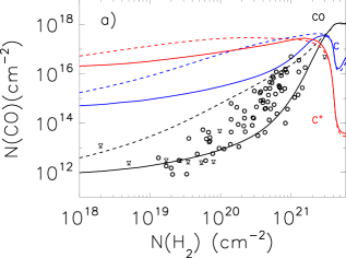
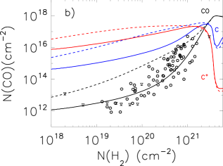
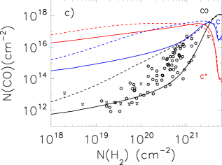
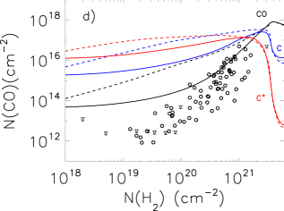
Figure 3: Column densities of CO(g) vs. H₂(g) for shock models 1 (panel a), 2 (panel b), 3 (panel c), and 4 (panel d). The solid lines represent models using the (A) parameters of $T_{\rm d,0}=15$ K, $E_{\rm A}=290$ K, while dashed lines represent models using the (B) parameters of $T_{\rm d,0}=20$ K, $E_{\rm A}=130$ K. Black lines represent CO(g), while the abundances of atomic C and C⁺ are represented as blue and red lines, respectively. Observed values of CO(g) appear as circles while upper limits appear as inverted triangles; both are compiled from a variety of sources listed in Section 5.

Our principal results are contained in two figures, in which we plot assorted column densities vs $A_{V}$ and $N[{\rm H_{2}}]$, respectively; the latter is more commonly used in studies of CO(g). The column densities of CO(g), $N$[CO(g)], and an assortment of ices are plotted against $A_{V}$ in Figure 2 for the A and B parameter sets and all four shock models. The column densities are shown for visual extinction through $A_{V}=3.3$, as further extensions of the evolution are definitely beyond the scope of the shock hydrodynamics (see discussion in B04 regarding the importance of gravity). The extinction used in Figure 2 is considered to be “edge-to-center” for a line of sight into dense or translucent material. Thus an observed extinction of 2 mag would correspond to 1 mag in the edge-to-center model frame. The column density for CO(g) is plotted against $N$[H₂] in Figure 3 along with column densities for the other major forms of carbon in the gas - C⁺ and C. In both figures, solid lines represent models with the A parameter set, while dashed lines represent the B set.

In each figure, it can be seen that the difference in $N$[CO(g)] between the A and B parameter sets decreases as the extinction or H₂ column increases. At low H₂ column, the amount of CO(g) produced in the B models apparently exceeds that in the A models by up to 2 orders of magnitude. This effect occurs primarily because the warmer grains produce less H₂(g) at a given $A_{V}$ with our simple “smooth” grain model; there is much less of a temperature dependence in the “rough” grain model of Chang et al. (2007), which utilizes a microscopic Monte Carlo approach. If the abscissa in Figure 3 were the column of total hydrogen rather than of just H₂, the B and A model results for CO(g) would appear to be more similar. Note also that the two plots with $N$[CO(g)] emphasize its growth with time in different ranges. In particular, the range of labeled $A_{\rm V}$ values in Figure 2 of 0.5-3.0 corresponds to only a small portion of the H₂ column density range in Figure 3.

Despite these complications, a salient feature of both figures is that CO(g) becomes the most abundant of the three major forms of carbon as $N[\rm{H_{2}}]\sim 4\times 10^{21}$ cm^-2 (corresponding to an edge-to-center $A_{V}\sim 2$). Thus, long before a cold core with $A_{\rm V}\sim 10$ forms, the carbon inventory in the gas phase contains large amounts of CO(g). Our results, obtained with a gas-grain model, are not identical with those of B04. Nevertheless, they confirm how artificial the initial carbon inventory is for pseudo-time-dependent models, in which carbon is assumed to be totally in its atomic ionic form while the density and visual extinction are already at their final values. Moreover, at a visual extinction of 2, the [C⁺ $+$ C]/[CO] abundance ratio is the same as we obtain at steady-state with a gas-phase model at roughly the same density. Thus, the system has already evolved into a translucent cloud.

In addition to CO(g), calculated column densities for the major ice species H₂O(s), CO(s), and CO₂(s), along with the somewhat less abundant ices CH₄(s) and CH₃OH(s), are shown in Figure 2. As illustrated in panel (b), the amount of H₂O(s) grows relatively quickly to column densities in excess of 10¹⁶ cm^-2 between $A_{V}=1.3$ and 2.1 for the various models. As with CO(g), the results illustrate that this occurs most efficiently for shock models with greater total density. The evolution of CO(s), as shown in panel (c), tends to lag behind CO(g), and the plot of its column vs $A_{\rm V}$ shows a sharp threshold at intermediate visual extinction, which is correlated with a decrease in the rate of synthesis of methanol (see below). The molecule forms more efficiently at lower extinction and earlier times for models with greater density, similar to the trend seen for H₂O(s).

There is a large distinction between models with the A and B parameters at low and intermediate visual extinction. For some molecular ices, specifically CO(s) and H₂O(s), as the visual extinction grows, the calculated column densities converge towards one another, while others show order of magnitude agreement (CH₄, CH₃OH). No convergence occurs for CO₂(s), as shown in panel (d), which requires the adoption of the B parameter set to achieve a significant column density, mainly because the warmer grains allow faster diffusive reaction processes for heavy species. Although the effects of individually varying the CO₂(s) formation barrier and turning off the Eley-Rideal mechanism on the abundance of CO₂(s) were considered, the grain temperature is the most influential parameter for CO₂(s) formation.

The formation of CO(g) and CO(s) also affects the evolution of methane ice (CH₄(s)) and methanol ice (CH₃OH(s)), shown in panels (e) and (f) of Figure 2, respectively. Methane on grain surfaces is formed via sequential hydrogenation of C atoms, which accrete from the gas. The less carbon and the more CO in the gas, the less efficient the surface formation of methane and the more CO(s) accretes onto grains. Even at an extinction of 3.0, the CH₄(s) column densities for individual models tend to lie below those of CO(s), especially for B parameter (warm grain) models. As regards methanol, its only formation is via sequential hydrogenation of CO(s) by reactions involving H atoms on grain surfaces:

$${\rm CO(s)\rightarrow HCO(s)\rightarrow H_{2}CO(s)\rightarrow H_{2}COH(s)\rightarrow CH_{3}OH(s),}$$ (2)

so that the abundances of CO(s) and CH₃OH(s) should be intimately tied together. Nevertheless, the extinction dependence of the column densities of methane and methanol is far more complex than that of CO(s), especially with the B parameters, where extra peaks are seen. For both CH₄(s) and CH₃OH(s) formation, warmer temperatures lead to more desorption of H atoms from the grains and would appear to slow down the hydrogenation of C(s) and CO(s). This factor clearly affects the formation of methane at most times, but runs counter to the observation that higher surface temperatures aid methanol formation and CO(s) depletion. Presumably this latter effect occurs because two of the reactions in the hydrogenation of methanol (H + CO and H + H₂CO) require overcoming a chemical reaction barrier.

In addition to the results shown in Fig. 2 and Fig. 3, we report additional results for major species at $A_{\rm V}$ = 3. Specifically, Table 2 contains the fractional abundances of the major gaseous and solid species for the A and B variants of Models 3 and 4. These models span the range of physical conditions considered, and the table illustrates the differences in composition that arise as a result. This table provides a range of input abundances for subsequent dense core models.

Table 2: Fractional Abundances of Major Species at $A_{V}=3$

Species/Model	3 A	3 B	4 A	4 B
Gas Phase
H2	0.5	0.5	0.5	0.5
H	7.2(-04)	7.4(-04)	1.1(-04)	1.1(-04)
CO	1.1(-04)	1.1(-04)	5.1(-05)	4.8(-05)
O	1.0(-04)	1.0(-04)	1.2(-05)	1.3(-05)
N2	2.9(-05)	3.2(-05)	3.1(-05)	3.2(-05)
N	2.5(-05)	2.1(-05)	4.0(-06)	4.5(-06)
S	8.7(-06)	8.9(-06)	6.0(-06)	6.2(-06)
S+	5.2(-06)	5.4(-06)	6.3(-07)	7.5(-07)
C	3.4(-06)	2.5(-06)	1.2(-06)	6.3(-07)
CS	4.0(-08)	2.1(-08)	6.9(-08)	2.8(-08)
CH4	1.8(-08)	4.9(-09)	2.2(-08)	2.7(-09)
C2H6	8.9(-09)	5.0(-08)	4.0(-09)	2.4(-08)
C+	8.8(-09)	6.7(-09)	5.6(-10)	4.3(-10)
CO2	2.2(-10)	1.1(-08)	1.7(-10)	4.1(-08)
Solid Phase
H2O(s)	4.7(-05)	4.2(-05)	1.4(-04)	1.2(-04)
CO(s)	9.9(-06)	1.1(-05)	6.8(-05)	6.7(-05)
NH3(s)	4.6(-06)	9.8(-07)	2.3(-06)	6.9(-07)
CH4(s)	4.4(-06)	5.6(-07)	5.0(-06)	2.7(-07)
H2S(s)	1.8(-06)	1.4(-06)	9.0(-06)	8.7(-06)
N2(s)	1.3(-06)	1.7(-06)	9.3(-06)	9.8(-06)
HCN(s)	1.0(-06)	1.2(-06)	3.7(-06)	1.5(-06)
MgH2(s)	4.2(-07)	4.3(-07)	6.1(-07)	6.2(-07)
SiH4(s)	4.7(-08)	5.3(-08)	4.6(-07)	4.6(-07)
FeH(s)	4.4(-08)	4.3(-08)	8.9(-08)	8.9(-08)
CH3OH(s)	4.0(-08)	2.2(-07)	2.5(-08)	1.3(-07)
C2H6(s)	2.8(-08)	1.3(-07)	1.7(-08)	9.4(-08)
H2CO(s)	2.4(-08)	1.3(-07)	1.5(-08)	7.6(-08)
SiO(s)	2.2(-08)	2.6(-08)	2.4(-07)	2.4(-07)
H2CS(s)	2.0(-08)	5.2(-08)	1.7(-08)	9.3(-08)
CO2(s)	9.7(-11)	7.8(-07)	2.9(-09)	1.1(-05)
H2O2(s)	7.8(-13)	8.0(-13)	8.8(-08)	5.7(-07)

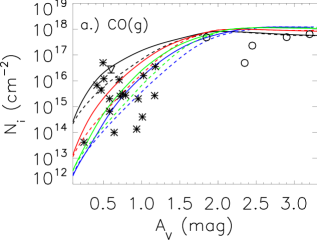
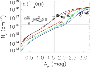
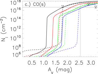
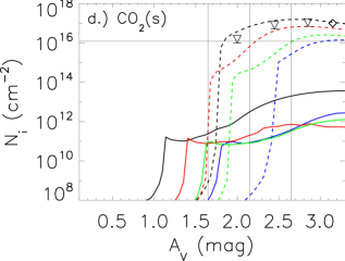
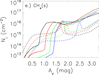
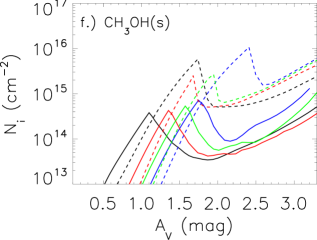
Figure 2: Column densities of selected molecules vs. visual extinction, for shock models 1 (green), 2 (red), 3 (blue), and 4 (black). The solid lines represent models using the (A) parameters of $T_{\rm d,0}=15$ K, $E_{\rm A}=290$ K, while dashed lines represent models using the (B) parameters of $T_{\rm d,0}=20$ K, $E_{\rm A}=130$ K. Observed ice values come from Whittet et al. (2007) (diamonds), Murakawa et al. (2000) (crosses), and Teixeira & Emerson (1999) (squares), while upper limits are included as inverted triangles. The observations of CO(g) come from Whittet et al. (1989) (circles) and from a variety of translucent cloud sources (see Section 5 for citations.) Vertical lines denote the threshold extinction $A_{\rm th}$ (Whittet et al. 2007) with estimated uncertainties; for CO(s) only the minimum value appears. The horizontal lines indicate estimated minimum column densities for detection (see Section 5).

Our results are obtained with a model that ignores grain growth. But, as grains accumulate icy mantles, the cross sections grow likewise, potentially by substantial factors. This effect is often omitted from gas-grain chemistry models. In the single grain-size model considered in this paper, the cross section gradually doubles following $A_{V}\gtrsim 1.5$. In some preliminary simulations with mantle growth, we found that the onset of CO(s) and CO₂(s) growth occurs at slightly lower $A_{V}$, and that these ices reach abundances slightly different from those of Fig. 2, while CO(g) and water ice decrease. Our overall results and conclusions are not changed significantly by consideration of this effect. The inclusion of mantle growth in a chemical model with a distribution of grain sizes is currently being undertaken by K. Acharyya and E. Herbst. In addition to mantle growth, the effect of grain-grain collisions can lead to size distributions with considerably larger grains at time scales such as those considered here, according to detailed calculations by Ormel et al. (2009) (see, in particular, their Table 3). Inclusion of this effect is beyond the scope of this paper.

5 Comparison with Observations

Although the density of the post-shock models can be as high as $2\times 10^{4}$ cm^-3, these do not simulate fully-formed dense cores given their low extinction, but rather the cloud material such as that from which dense cores form. Can relevant comparison be made with existing observational data, or are our results best used as initial conditions for models of normal dense cold cores? The dark cloud in Taurus is perhaps the best region to explore this question for measurements of ices, while a large sample of CO(g) observations exists for diffuse and translucent clouds, as well as some lines of sight in Taurus. One must also remember that our results represent cold material in the act of forming larger structures via a specific post-shock process, whereas there is no guarantee that the observed sources are transitional in this sense. Indeed, at low visual extinction and/or H₂ column densities, our objects tend to be denser, smaller, and colder than well-studied diffuse clouds.

5.1 CO(g) Observations

Estimates of $N$[CO(g)] along darker lines of sight in the Taurus dark cloud were presented by Whittet et al. (1989) based on observations of Frerking et al. (1982) and Crutcher (1985). Observations of $N$[CO(g)] in more translucent and diffuse clouds have been reported by Liszt (2008); Burgh et al. (2007); Sheffer et al. (2007); Sonnentrucker et al. (2007); Gredel et al. (1994), and references therein. The value of $A_{V}$ was reported for some of these sources by Rachford et al. (2009), while for the majority only $N$[H₂(g)] was reported.

The $N[\rm{CO(g)}]$ vs. $A_{V}$ data appear in Figure 2(a) as circles for the darker lines of sight, seen in the Taurus cloud, and asterisks for the translucent lines of sight except for one upper limit, shown as an inverted triangle. It is apparent from this figure that many of the data points fall within the model curves in the lower $A_{V}$ range, and that all four shock models with A and B parameter sets fit three of the darker line of sight observations to within a factor of 3 or better.

The $N$[CO(g)] vs. $N$[H₂(g)] data appear in Figure 3 as either circles or inverted triangles for upper limits. The data, which are more numerous than those plotted against $A_{\rm V}$ and tend to contain lower CO(g) columns from diffuse and translucent cloud data, are fit best by model 2-A. The B-models tend to be somewhat worse than the A-models. Although the density, gas temperature, and size of the post-shock objects for the lower H₂ columns may not correspond with these parameters for actual observed clouds, the CO(g) columns we calculate are dependent mainly on the visual extinction, so observation and theory are in reasonable agreement anyway. In addition, the calculated CO(g) columns agree well with steady-state values for gas-phase models, if not quite as well as in Figure 2.

5.2 Ice Observations

Our predicted column densities for ices as functions of edge-to-center visual extinction can be compared with at least some infrared observational data along quiescent lines of sight in Taurus in our low visual extinction regime. Shown in Figure 2, the limited data available in the extinction range up to 3.3 come from Whittet et al. (2007); Murakawa et al. (2000); Teixeira & Emerson (1999), and references therein. Some of these data are merely upper limits, while for CH₄(s) and CH₃OH(s), there are to the best of our knowledge not even upper limits in this range. The question arises as to whether observations at our relatively low extinction range belong to small cores or whether the material being sampled is simply the diffuse background. That at least some of the Taurus observations at low extinction pertain to small cores has been shown by Whittet et al. (2001, 2004), who concluded that the lines of sight to HD 29647 and HD 283809 sample dense gas with extinctions of $A_{V}=1.82$ and 2.85 (see their Figure 1 in the 2004 paper). If representative of expanding objects as treated by our shock model, the size of the object with lower extinction, in the absence of self-gravity, would be in the range 0.05 pc (Model 4) to 0.5 pc (Model 3) (see Table 1).

The vertical line or lines in panels (b)-(d) are empirically determined threshold extinctions, $A_{\rm th}$, and their uncertainty ranges for the Taurus dark cloud (the panel for CO(s) only shows the lower limit of this range). The center lines represent the lowest $A_{V}$ values above which the specific ices are detectable in a cloud and are obtained by empirical fits to column density vs. visual extinction for a wide range of dark quiescent lines of sight in Taurus towards background stars at larger visual extinction (Whittet et al. 2007). The specific edge-to-center thresholds for Taurus are $A_{\rm th}=1.6\pm 0.05$ for H₂O(s), $3.4\pm 0.8$ for CO(s), and $2.15\pm 0.5$ mag for CO₂(s). These threshold values can be regarded as conservative compared with some of the equivocal data at lower extinction from other groups (Teixeira & Emerson 1999; Murakawa et al. 2000), which might represent the diffuse background. The thresholds are thought to roughly correspond with the accumulation of the equivalent of a few monolayers of a surface species, in a sudden onset above the threshold extinction. To help interpret these thresholds, we have also plotted minimum detectable columns for the major ices, which are shown as horizontal lines. The estimates are made by substituting a minimal discernible optical depth of $\tau=0.01$ (Whittet, private communication) into equation (5.5) of Whittet (2003). At the time when $A_{V}\approx A_{\rm th}$, the horizontal lines in panels (b) and (d) represent the equivalent column density of about one or two monolayers of H₂O(s) and CO₂(s), while the line in panel (c) is closer to five layers of CO(s).

The observations of $N$[H₂O(s)] appear in Figure 2(b). The Murakawa et al. detections were reported as optical depths, $\tau$, and we note that several of these values are less than the observational uncertainty of $\delta\tau=\pm 0.05$ reported. If we instead count these points as upper limits, as shown in the plot, the data below Whittet’s threshold range are only limits, while firm detections appear at greater $A_{\rm V}$ than the threshold. Below the threshold, the models results lie below these “limits.” Above the threshold, the spread of data points and upper limits falls within the range of our model results, although it is difficult to determine which models are best. Regarding the threshold itself, our calculated columns do not show a real threshold, but rise gradually and reach the empirical threshold around the minimum detectable column (the horizontal line). A proper interpretation may be that there is not really a threshold, so much as a drop below detectability masquerading as one. Towards the highest extinction plotted, the assorted model results tend to converge to a narrow range of values 3-10 $\times$ larger than the observed columns. In some sense this is due to the chemistry readily hydrogenating oxygen atoms on grain surfaces. At cold temperatures it is difficult to stop this process. The difference between model and observations could be related to our assumed oxygen atom abundance being too high, perhaps through the presence of another reservoir of oxygen (see, e.g. Whittet et al. 2007).

.

For the other major ices, CO(s) and CO₂(s), there are only upper limits in the extinction range $A_{\rm V}$ through $\approx 3$, except for one detection of CO₂(s) toward Tamura 2 (Whittet et al. 1989, 2007). The observational $N$[CO(s)] upper limits are not very constraining except perhaps at the highest visual extinction plotted where two upper limits are in better agreement with shock models 1 and 3. For the case of CO₂(s), the B parameter models are required to bring the column density to near-detectable abundances. The one firmly detected observational data point is fit best by models 4-B and 2-B.

Figure 2 shows very sharp thresholds for the onset of column densities of CO(s) and CO₂(s), but only for the latter are the calculated thresholds even in rough agreement with the empirical range of Whittet et al. (2007). For CO(s), we reach the minimum detectable column at visual extinction much smaller than the empirical threshold, which needs to be checked by data at lower extinction, where there are currently only high upper limits to the CO(s) column. It should be noted that, in the absence of photodesorption, minimum detectable columns for H₂O(s) and CO(s) are reached at lower visual extinction ($A_{V}\lesssim 1$), worsening the agreement with the threshold observations.

6 Discussion

The chemistry of cold dense cores has typically been treated by pseudo-time-dependent methods, in which physical conditions are homogeneous and time-independent. Also, the initial chemical abundances are artificially assumed to take the form of atoms except for molecular hydrogen. Although such gas-phase and gas-grain models of the chemistry are often in reasonable agreement with observations and even predictive in nature for the gas-phase species, the assumption of time-independent physical conditions ignores the formation of the core, a process that cannot be totally distinct from the chemistry that occurs. For these reasons, we have started a program to determine how the chemistry is altered by consideration of the physical evolution of dense cores.

In this paper, we have reported our study of the chemistry that occurs during shock-induced formation of dark cloud material from the more diffuse background, with an emphasis on the composition of icy grain mantles and gaseous CO. In this picture, gas-phase and grain-mantle molecular species form after the post-shock material cools and becomes dense, and as the visual extinction increases, in contrast with the assumption of constant physical conditions. This stage can be considered as preliminary to the stage in which cold pre-stellar cores form. Since our approach does not extend to the phase in which the self-gravity governs the evolution of these cooled objects, we cannot continue to increase their size and visual extinction beyond an extinction of $\approx 2-3$. Although our calculated column densities cannot then be compared with those of ordinary cold dense, or prestellar, cores, we have compared them with the observed abundances of diverse low-$A_{V}$ sources within the Taurus dark cloud, and a variety of other diffuse-to-translucent sources.

There are several key results of our calculations:

1. Despite some divergence at lower extinction, all model results for CO(g) tend to converge as the edge-to-center extinction reaches $\sim 2.0$ (an H₂ column of $4\times 10^{21}$ cm^-2) where CO(g) becomes the dominant form of gaseous carbon. We conclude that homogeneous gas-grain dense core models should not use atomic carbon as an initial abundance, but would be more realistic with initial abundances from the low-extinction results reported here. In particular, the calculated CO(g) columns and [C⁺ + C]/CO ratios for the different models are not drastically different from the values obtained from gas-phase models at steady-state as a function of visual extinction or molecular hydrogen column density. Our suggestion concerning the proper initial abundances to use has also appeared in a recent paper by Liszt (2009), who advocated that “mechanisms for the chemical evolution from diffuse to dark gas should be included in model calculations”, a view that is the basis for our paper.

2. By $A_{V}=2.5$, all models show that H₂O(s) and CO(s) have grown above their minimum observable abundances. Models that form denser gas grow these ices at lower $A_{V}$. These ices thus become abundant before a full-fledged dense core can be produced.

3. The growth of CO(s) slows down the rate of synthesis of CH₄(s) because there is less of its precursor, neutral C, available. By an extinction of 3.0, the methane column densities for individual models tend to lie below those of CO(s), especially for the B parameter set, in which the dust temperature is higher.

4. The formation of CO₂(s) occurs efficiently only with the B parameter models, especially with the higher density models, 2-B and 4-B. The grain temperature is the most critical parameter for efficient CO₂(s) formation, with or without the Eley-Rideal mechanism.

5. Models excluding photodesorption rates would form multiple layers of H₂O(s) and CO(s) at lower $A_{V}$ than either thresholds or the lowest reported firm detections (Whittet et al. 2007). This result indicates that the inclusion of measured photodesorption rates is critical for realistic models.

Finally, and most importantly, our results show that if the shock model of B04 is correct, the early stages of both gas-phase and grain-surface chemistry occur as dense material is being formed, so that the chemistry of the cold cores that form from the final collapse of dense material should betray some indications of the physics of core formation. Models that follow the chemistry as the dark cloud material formed in our model collapses to produce dense pre-stellar cores are desirable. In addition, other dynamical scenarios than our shock model do exist, and we hope to explore them.