Geothermal Casimir phenomena for the sphere-plate and cylinder-plate configurations

Abstract

We investigate the nontrivial interplay between geometry and temperature in the Casimir effect for the sphere-plate and cylinder-plate configurations. At low temperature, the thermal contribution to the Casimir force is dominated by this interplay, implying that standard approximation techniques such as the PFA are inapplicable even in the limit of small surface separation. Thermal fluctuations on scales of the thermal wavelength lead to a delocalization of the thermal force density at low temperatures. As a consequence, the temperature dependence strongly differs from naive expectations. Most prominently, thermal forces can develop non-monotonic behavior below a critical temperature. We perform a comprehensive study of such geothermal phenomena in these Casimir geometries, using analytical and numerical worldline techniques for Dirichlet scalar fluctuations.

I Introduction

The Casimir effect [1], inspiring many branches of physics [2, 3], features a decisive geometry dependence: the fluctuation-induced interaction between test bodies or surfaces depends on their shape and orientation. This is because the Casimir effect arises from the fluctuation spectrum in presence of the surfaces relative to the vacuum fluctuations. The spectral properties in turn are a direct consequence of the geometry.

This geometry dependence becomes even more pronounced at finite temperature $T$: thermal fluctuations can predominantly be associated with a characteristic length scale, the thermal wavelength $\lambda_{T}\sim\hbar c/(k_{\text{B}}T)$. Thermal fluctuations contribute to the Casimir force, whenever the scale set by the thermal wavelength is commensurate with a mode of the fluctuation spectrum as defined by the geometry. Therefore, thermal corrections to the zero-temperature Casimir effect generally cannot be described by universal additive terms or other simple recipes but require a careful analysis of the interplay between geometry and temperature, as first anticipated in [4].

This “geothermal” interplay has first been verified in paradigmatic perpendicular-plates [5] or general inclined-plates configurations [6]. Further evidence for the experimentally relevant sphere-plate configuration has been provided recently in [7, 8, 9, 10]. Typical low-temperature dependencies in these open geometries obey power laws with characteristic exponents that are particular for the geometry. Most importantly, these power laws disagree with predictions from standard local approximation techniques such as the proximity force approximation (PFA) [11] – even in the limit of vanishing surface separation. This is in contrast to zero-temperature forces which are often well described by the PFA in this limit [12].

In this work, we perform a comprehensive study of the geometry-temperature interplay for the sphere-plate and cylinder-plate configuration. We study the Casimir forces induced by fluctuations of a scalar field obeying Dirichlet boundary conditions on the surfaces in order to explore the geothermal interplay in a most transparent fashion. Moreover, we use the worldline approach to the Casimir effect [13] which on the one hand provides for a highly intuitive picture of the fluctuations, and on the other hand facilitates analytical as well as numerical computations from first principles [14, 15, 16, 17].

For instance, the failure of local or additive approximation techniques can directly be inferred from the temperature dependence of the force density: the latter tends to delocalize for decreasing temperatures on scales of the thermal wavelength [8]. Local approximation techniques may only be useful at finite temperature if the strict weak-coupling limit is taken [18], or in the high-temperature limit.

In the present work, we analyze the thermal force density distributions, compute thermal forces for a wide nonperturbative range of parameters, and determine asymptotic limits. This facilitates a careful comparison with local approximation techniques, and, most importantly, yields new and unexpected results for the geometry dependence of thermal forces. For instance, the pure thermal force, i.e., the thermal contribution to the Casimir force, reveals a non-monotonic behavior below a critical temperature for the sphere-plate and cylinder-plate case [19]: the attractive thermal force can increase for increasing distances. This anomalous feature is triggered by a reweighting of relevant fluctuations on the scale of the thermal wavelength – a phenomenon which becomes transparent within the worldline picture of the Casimir effect. Whereas these non-monotonic features already occur for a simple Dirichlet scalar model, non-monotonicities can also arise from a competition between TE and TM modes of electromagnetic fluctuations in configurations with side walls [20, 21].

While there are a number of impressive verifications of the zero-temperature Casimir force [22], a comparison between theory and thermal force measurements suffers from the interplay between dielectric material properties and finite temperature [23], still being a subject of intense theoretical investigations [24, 25, 26, 27, 28, 29]. In view of the geothermal interplay, we expect that the full resolution of this issue requires the comprehensive treatment of geometry, temperature and material properties, possibly also including edge effects [31, 30, 6, 32, 33]. First results on the sphere-plate configuration using scattering theory and specific dielectric models demonstrate this nontrivial interplay [34, 7, 10].

As a crucial ingredient for such an analysis, field-theoretical methods for Casimir phenomena have to be used that can deal with arbitrary Casimir geometries. In addition to the worldline methods [13, 35, 36, 37, 38] used in this work, a variety of approaches has been developed in recent years, such as a functional integral approach [39, 40, 41] and scattering theory [42, 43, 44, 45, 46, 47, 48, 49, 50]. An extension of these methods to finite temperature is usually straightforward and highly worthwhile in view of the geometry-temperature interplay.

Our paper is organized as follows: after a brief account of the worldline approach to the Casimir effect in Sect. II, the sphere-plate and cylinder-plate configurations are studied at zero temperature in Sect. III. In addition to making contact with the literature, we perform the worldline computation directly for the force instead of the interaction energy. Section IV contains all our main results on the finite-temperature case. Our conclusions are summarized in Sect. V. For reasons of comparison, the proximity-force approximation for the sphere-plate and cylinder-plate case is worked out in detail in appendix A. In addition to explicit formulas which have not comprehensively appeared in the literature so far, we relate the PFA to an approximate treatment of the worldline path integral which helps to understand the differences between the exact and approximate treatments.

II Worldline approach to the Casimir effect

We start with a short reminder of the worldline approach to the Casimir effect for a massless Dirichlet scalar in 4 dimensions; for details, see [13, 37, 6]. For a configuration $\Sigma$ consisting of two rigid objects with surfaces $\Sigma_{1}$ and $\Sigma_{2}$, the worldline representation of the Casimir interaction energy in $D=4$ dimensional spacetime reads

$$E_{\mathrm{c}}=-\frac{1}{32\pi^{2}}\!\int_{0}^{\infty}\frac{\mathrm{d}\mathcal{T}}{\mathcal{T}^{3}}\!\int\!\mathrm{d}^{3}x_{\mathrm{CM}}\left\langle\Theta_{\Sigma}[\mathbf{x}(\tau)]\right\rangle.$$ (1)

The worldline functional $\Theta_{\Sigma}[\mathbf{x}(\tau)]$ is $1$ if the worldline $\mathbf{x}(\tau)$ intersects both objects $\Sigma=\Sigma_{1}\cup\Sigma_{2}$, and is zero otherwise.

The expectation value in Eq. (1) is taken with respect to an ensemble of $3$-dimensional closed worldlines with a common center of mass $\mathbf{x}_{\mathrm{CM}}$ and obeying a Gaußian velocity distribution. For static Casimir configurations the time component cancels out at zero temperature. Equation (1) has an intuitive interpretation: All worldlines intersecting both surfaces violate Dirichlet boundary conditions and are removed from the ensemble of allowed fluctuations, contributing to the negative Casimir interaction energy. During the ${\mathcal{T}}$ integration, the extent of a worldline is scaled by $\sqrt{\mathcal{T}}$ . Large propertimes $\mathcal{T}$ correspond to IR fluctuations, small $\mathcal{T}$ to UV fluctuations.

Introducing finite temperature $T=1/\beta$ by the Matsubara formalism is equivalent to compactifying Euclidean time on the interval $[0,\beta]$. The Casimir free energy corresponding to Eq. (1) now becomes

$$E_{\mathrm{c}} = -\frac{1}{32\pi^{2}}$$

$$\times\!\!\int_{0}^{\infty}\frac{\mathrm{d}\mathcal{T}}{\mathcal{T}^{3}}\!\!\sum_{n=-\infty}^{\infty}\!\!e^{-\frac{n^{2}\beta^{2}}{4\mathcal{T}}}\!\!\int\!\mathrm{d}^{d}x_{\mathrm{CM}}\left\langle\Theta_{\Sigma}[\mathbf{x}(\tau)]\right\rangle.$$

For numerical purposes, it is convenient to remove the $\mathcal{T}$ dependence from the velocity distribution by the rescaling

$$\bm{\gamma}(t):=\frac{1}{\sqrt{\mathcal{T}}}\mathbf{x}(\mathcal{T}t)\quad\!\!\!\to\!\!\!\quad e^{-\frac{1}{4}\int_{0}^{\mathcal{T}}\dot{\mathbf{x}}^{2}\mathrm{d}\tau}=e^{-\frac{1}{4}\int_{0}^{1}\dot{\bm{\gamma}}^{2}\mathrm{d}t},$$ (3)

where $\dot{\bm{\gamma}}=\mathrm{d}\bm{\gamma}(t)/\mathrm{d}t$. Now, the $\Theta$ function reads more explicitly

$$\Theta[\mathbf{x}]\equiv\Theta[\mathbf{x}_{\text{CM}}+\sqrt{\mathcal{T}}\bm{\gamma}(t)].$$ (4)

The worldline integrals are evaluated numerically by Monte Carlo methods, i.e, the path integral is approximated by a sum over a finite ensemble of ${n_{\text{L}}}$ worldlines. Each worldline $\bm{\gamma}(t)$ is furthermore discretized by a finite set of $N$ points per loop (ppl). To generate discretized worldlines with Gaußian velocity distribution the v-loop algorithm was used in this work [13, 51]. In the remainder, we apply the worldline method to the sphere-plate and cylinder-plate Casimir configurations.

III Casimir effect at zero temperature

Let us first study the sphere-plate and cylinder-plate geometries at zero temperature. Here, we make contact with earlier results for the Casimir effect of a cylinder and sphere above a plate [17, 42, 36, 43, 44, 37]. Moreover, we generalize the worldline method to directly compute the Casimir force instead of the energy which leads again to significant simplifications compared to previous energy calculations. The method will be generalized to finite temperature in the next section.

III.1 Sphere above a plate

We start the configuration of a sphere above a plate. The sphere of radius $R$ is centered around the origin $\mathbf{x}=0$. The infinitely extended plate lies in the $z=-(a+R)$ plane, where $a$ is the minimal distance between both objects, see Fig. 1. Since the configuration has a rotational symmetry with respect to the $z$ axis, the three dimensional $\mathbf{x}_{\mathrm{CM}}$ integration reduces to a two dimensional one. The Casimir energy (1) reads

$$E_{\mathrm{c}}=-\frac{1}{16\pi}\!\int_{0}^{\infty}\frac{\mathrm{d}\mathcal{T}}{\mathcal{T}^{3}}\!\int\!\mathrm{d}r\,\mathrm{d}z_{\mathrm{CM}}\,r\left\langle\Theta_{\Sigma}[\mathbf{x}(\tau)]\right\rangle,$$ (5)

where we have switched to cylindrical coordinates ($r,z_{\mathrm{CM}}$) with $r^{2}=x_{\mathrm{CM}}^{2}+y_{\mathrm{CM}}^{2}$. The $\Theta_{\Sigma}[\mathbf{x}(\tau)]$ functional factorizes,

$$\Theta_{\Sigma}[\mathbf{x}(\tau)]=\Theta_{\mathrm{S}}[\mathbf{x}_{\mathrm{CM}}+\sqrt{\mathcal{T}}\bm{\gamma}]\Theta_{\mathrm{P}}[\mathbf{x}_{\mathrm{CM}}+\sqrt{\mathcal{T}}\bm{\gamma}].$$ (6)

Here $\Theta_{\mathrm{S}}$ and $\Theta_{\mathrm{P}}$ account for the intersection of a worldline $\mathbf{x}_{\mathrm{CM}}+\sqrt{\mathcal{T}}\bm{\gamma}$ with the sphere and the plate, respectively. Notice that $\Theta_{\mathrm{S}}$ is independent of $a$, whereas $\Theta_{\mathrm{P}}$ reads

$$\Theta_{\mathrm{P}}=\theta(-(a+R+z_{\mathrm{CM}}+\sqrt{\mathcal{T}}\bm{\gamma}_{z_{\mathrm{min}}})),$$ (7)

where $\bm{\gamma}_{{z_{\mathrm{min}}}}$ denotes the worldline’s extremal extent into the negative $z$ direction.

As we are interested in calculating the Casimir force, $F_{\mathrm{c}}=-\mathrm{d}E_{\mathrm{c}}/\mathrm{d}a$, the derivative acting only on $\Theta_{\mathrm{P}}$ produces a $\delta$ function which eliminates the $z_{\mathrm{CM}}$ integral. The Casimir force thus simplifies to

$$F_{\mathrm{c}}=-\frac{1}{16\pi}\,\left\langle\int_{0}^{\infty}\frac{\mathrm{d}\mathcal{T}}{\mathcal{T}^{3}}\int_{0}^{\infty}\mathrm{d}r\,r\,\Theta_{\mathrm{S}}[\widetilde{\mathbf{x}}+\sqrt{\mathcal{T}}\ \widetilde{\bm{\gamma}}]\right\rangle.$$ (8)

Here, we have introduced

$$\widetilde{\mathbf{x}}=\left(\begin{array}[]{c}r\\ 0\\ -a-R\\ \end{array}\right),\ \ \ \ \ \ \widetilde{\bm{\gamma}}=\left(\begin{array}[]{c}\bm{\gamma}_{x}\\ \bm{\gamma}_{y}\\ \bm{\gamma}_{z}-\bm{\gamma}_{z_{\mathrm{min}}}\\ \end{array}\right).$$ (15)

The transition from worldline calculations of the force does not only lead to technical simplifications. Also, the classification of relevant worldlines changes slightly: for the Casimir energy in Eq. (1) the worldlines are scaled by the propertime $\sqrt{\mathcal{T}}$ with respect to their center of mass which is finally integrated over. For a given center of mass, all points on a worldline $\mathbf{x}_{\mathrm{CM}}+\sqrt{\mathcal{T}}\bm{\gamma}(t_{i})$ lie on rays originating from the center of mass. These rays are traced out by the $\mathcal{T}$ integral running from $\mathcal{T}=0$ to $\mathcal{T}=\infty$.

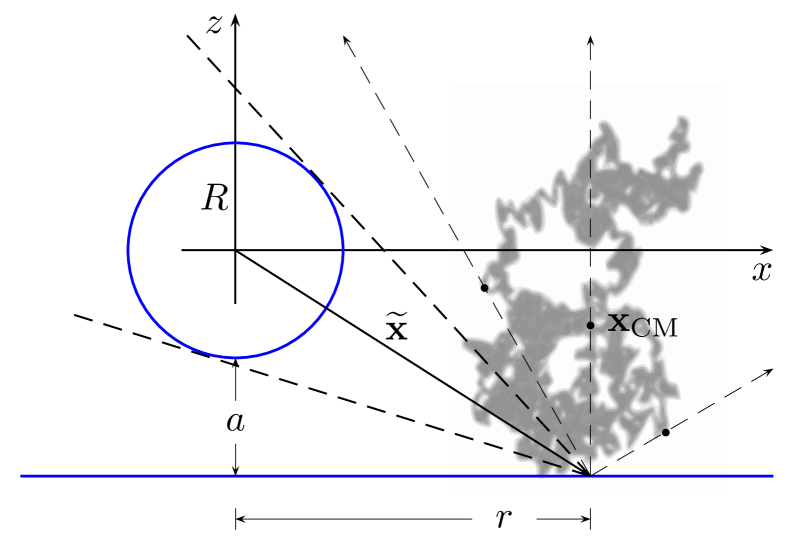
Figure 1: Sketch of the sphere-plate configuration. The infinite plate (blue line) is in the $z=-(R+a)$ plane. The sphere of radius $R$ is in the origin. The center of mass $\mathbf{x}_{\mathrm{CM}}$ of the worldline is in $(r,0,-a-R-\sqrt{\mathcal{T}}\bm{\gamma}_{z_{\mathbf{\min}}})$. During the propertime integration the worldline always touches the plate, while all its points move on rays passing through $(r,0,-a-R)$. Only points lying inside the cone will pass through the sphere.

By contrast, the Casimir force in Eq. (8) results from worldlines which are attached to the point $\widetilde{\mathbf{x}}$ on the plate. For a given point $\widetilde{\mathbf{x}}$, all points on a worldline $\widetilde{\mathbf{x}}+\sqrt{\mathcal{T}}\,\widetilde{\mathbf{\bm{\gamma}}}(t_{i})$ lie on rays which now originate from $\widetilde{\mathbf{x}}$. Again these rays are traced out by the $\mathcal{T}$ integral.

Now, the plate is always touched by by construction for all values of $\mathcal{T}$, the remaining problem being the detection of intersection events with the sphere. Adapting methods from [37], it is clear that only those points of a worldline lying on the rays intersecting the sphere eventually pass through the sphere for some values of $\mathcal{T}$. Let $\{\widetilde{\bm{\gamma}}(t_{k})\}$ denote the set of points on such rays intersecting the sphere, with $k$ labeling these rays for a discretized worldline. Those values of propertime $\mathcal{T}$ for which this point lies exactly on the sphere can be obtained from the equation

$$(\widetilde{\mathbf{x}}+\sqrt{\mathcal{T}}\,\widetilde{\bm{\gamma}}(t_{k}))^{2}=R^{2}.$$ (16)

Equation (16) has two solutions,

$$\mathcal{T}^{\pm}_{k}=\left(\frac{\widetilde{\mathbf{x}}\cdot\widetilde{\bm{\gamma}}(t_{k})}{|\widetilde{\bm{\gamma}}(t_{k})|^{2}}\mp\sqrt{\left(\frac{\widetilde{\mathbf{x}}\cdot\widetilde{\bm{\gamma}}(t_{k})}{|\widetilde{\bm{\gamma}}(t_{k})|^{2}}\right)^{2}-\frac{|\widetilde{\mathbf{x}}|^{2}-R^{2}}{|\widetilde{\bm{\gamma}}(t_{k})|^{2}}}\right)^{2}.$$ (17)

For $\mathcal{T}\in(\mathcal{T}^{-}_{k},\,\mathcal{T}^{+}_{k})$ the point $\widetilde{\mathbf{x}}+\sqrt{\mathcal{T}}\,\widetilde{\bm{\gamma}}(t_{k})$ lies inside the sphere. The point $\widetilde{\mathbf{x}}$ can be viewed as a tip of a cone that wraps around the sphere with the opening angle $2\alpha$, with $\sin(\alpha)=R/|\widetilde{\mathbf{x}}|$. The value of the square root in Eq. (17) varies between zero and $R$. The square root is zero if the ray merely touches the sphere, and $R$ if the ray lies on the cone’s axis, i.e., if it coincides with the direction spanned by $\widetilde{\mathbf{x}}$.

For a given $r$, the worldline intersects the sphere if the propertime $\mathcal{T}$ is in one of the intervals bounded by Eq. (17) for all possible values of $k$. Denoting these intervals by $\overline{\mathcal{T}}_{k}:=[\mathcal{T}^{-}_{k},\,\mathcal{T}^{+}_{k}]$. The total support of the propertime integral then is

$$\mathcal{S}(r) =\bigcup_{k}\overline{\mathcal{T}}_{k}.$$ (18)

The $r$ dependence of this support arises from the fact that the set of $k$ rays lying inside the cone depends on the position $r$ where the worldline is attached to the plate. The Casimir force (6) now reads

$$F_{\mathrm{c}}=-\frac{1}{16\pi}\,\left\langle\int_{0}^{\infty}\mathrm{d}r\,r\int_{\mathcal{S}(r)}^{\infty}\frac{\mathrm{d}\mathcal{T}}{\mathcal{T}^{3}}\ \right\rangle.$$ (19)

The most time-consuming part of the algorithm is the determination of $S(r)$ if the distance between the sphere and plate is small. To reduce the computational time, it is advisable to reduce the $N$ points per worldline to the subset of $k<N$ points on the above mentioned rays intersecting the sphere. For a given $r$, all points on rays outside the cone can immediately be dropped. Furthermore in the process of taking the $r$ integral from zero to infinity, the opening angle of the cone shrinks. All points on rays which leave the cone through its upper half can then be dropped completely from the calculation, as they will never enter the cone again. Only rays below the cone, i.e., between the cone and the plate, can enter the cone for larger values of $r$. With these optimizations and with one integral less, the computational time for Casimir force calculations is significantly reduced compared with those of the Casimir energies studied in previous worldline investigations.

These simplification facilitate to extend the previously studied parameter range to even larger $a/R$ ratios with higher statistics.

III.2 Cylinder above a plate

In many respects, the cylinder-plate configuration is “in between” the sphere-plate configuration and the classic parallel-plates case. This also holds for the experimental realization: the effort of keeping the cylinder parallel to the plate is less than it is the case for two parallel plates [52]; for the sphere-plate case, this issue is simply absent. As a clear benefit, the force can, in principle, be made arbitrarily large, since it is proportional to the length of the cylinder.

The geometry of the cylinder-plate configuration can be parameterized analogously to the preceding sphere-plate case: we consider the symmetry axis of a cylinder of an (infinite) length $L_{y}$ and radius $R$ to coincide with the $y$ axis. The infinite plate lies in the $z=-(R+a)$ plane, with $a$ being the distance between the cylinder and the plate.

The Casimir force can be obtained directly from Eq. (1), where use the fact that the $\Theta_{\Sigma}[\mathbf{x}(\tau)]$ functional factorizes (cf. Eq. (6))

$$\Theta_{\Sigma}[\mathbf{x}(\tau)]=\Theta_{\mathrm{Cyl}}[\mathbf{x}_{\mathrm{CM}}+\sqrt{\mathcal{T}}\bm{\gamma}]\Theta_{\mathrm{P}}[\mathbf{x}_{\mathrm{CM}}+\sqrt{\mathcal{T}}\bm{\gamma}].$$ (20)

Here $\Theta_{\mathrm{Cyl}}$ and $\Theta_{\mathrm{P}}$ account for the intersection of a worldline $\mathbf{x}_{\mathrm{CM}}+\sqrt{\mathcal{T}}\bm{\gamma}$ with the cylinder and the plate, respectively. Again, only $\Theta_{\mathrm{P}}$ depends on $a$ and is given in Eq. (7).

The $y$ integral in the Casimir energy (1) is now trivial due to translational symmetry. The Casimir force can then be obtained directly from Eq. (8) and reads

$$F_{\mathrm{c}}=\frac{L_{y}}{16\pi^{2}}\,\left\langle\int_{0}^{\infty}\frac{\mathrm{d}\mathcal{T}}{\mathcal{T}^{3}}\int_{0}^{\infty}\mathrm{d}r\ \Theta_{\mathrm{Cyl}}\left[\widetilde{\mathbf{x}}+\sqrt{\mathcal{T}}\ \widetilde{\bm{\gamma}}\right]\right\rangle,$$ (21)

where $r=|x_{\mathrm{CM}}|$ and

$$\widetilde{\mathbf{x}}=\left(\begin{array}[]{c}r\\ -a-R\\ \end{array}\right),\ \ \ \ \ \ \widetilde{\bm{\gamma}}=\left(\begin{array}[]{c}\bm{\gamma}_{x}\\ \bm{\gamma}_{z}-\bm{\gamma}_{z_{\mathrm{zmin}}}\\ \end{array}\right).$$ (26)

As in the case of the sphere, the worldlines $\widetilde{\mathbf{x}}+\sqrt{\mathcal{T}}\,\widetilde{\bm{\gamma}}$ are attached to the plate at the point $\widetilde{\mathbf{x}}$. The only difference is that the worldlines are now $2$ dimensional – a fact which reduces the computational cost. Only those points of a worldline lying on the rays intersecting the cylinder pass through the latter for some values of $\mathcal{T}$. The construction of the support of the $\mathcal{T}$ integral is identical to that for the sphere-plate case, such that the total Casimir force on the cylinder can be written as in Eq. (19)

$$F_{\mathrm{c}}=-\frac{L_{y}}{16\pi^{2}}\ \int_{0}^{\infty}\mathrm{d}r\left\langle\int_{\mathcal{S}(r)}\frac{\mathrm{d}\mathcal{T}}{\mathcal{T}^{3}}\right\rangle.$$ (27)

III.3 Zero-temperature results for the Casimir force

It is instructive to compare our results not only with analytic estimates, but also with the much simpler proximity force approximation (PFA). The latter is used by default for the data analysis of geometry corrections in most experiments. It derives from a classical reasoning for generalizing the parallel-plate case; thus, deviations of the exact result from the PFA estimate also parameterize genuine geometry-induced quantum behavior.

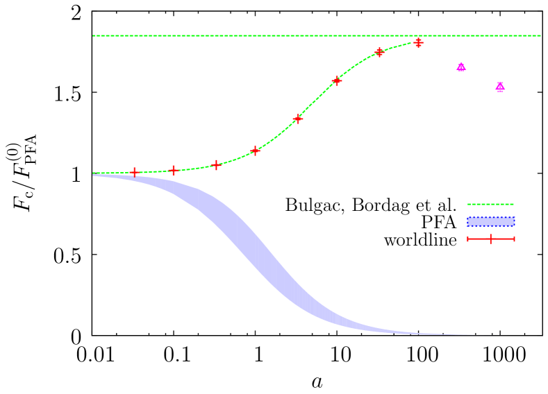
Figure 2: Casimir Force of a sphere of radius $R=1$ above an infinite plate vs. the distance $a$. The force is normalized to the zeroth-order PFA formula. We observe an excellent agreement with the exact asymptotic solutions for small $a$ [44] and for large $a$ [42] up to $a=100$. For larger $a$, the number of $N$ points per loop has to be increased far beyond $N=2\cdot 10^{7}$ used for this plot; otherwise, the sphere falls through the rough mesh provided by the insufficiently discretized worldline, leading to a systematically underestimated force as is visible here for $a>100$ (pink triangles).

Roughly speaking, the PFA subdivides the surfaces into small surface elements, applies the parallel-plate force or energy law to pairs of surface elements and integrates the resulting force density. The PFA is inherently ambiguous as the measure for this final integration is not unique: possible alternatives are the surface measures of one of the involved surfaces or any intermediate auxiliary surface. Later on, we will refer to the “sphere-based” or “plate-based” PFA as two generic options for the integration measure. The PFA for the present configuration is discussed in detail in Appendix A.

The concept of the PFA can also be translated into the worldline picture: as an approximation to the ensemble of complicated multidimensional worldlines, we may reduce the worldlines to one dimensional straight lines. The length of a line then corresponds to the average extent of a worldline into a certain relevant direction in a given geometry. This picture also explains the occurrence of deviations from the PFA as well as the sign of these deviations in the Dirichlet case: due to the spatial extent of the worldlines, they generically intersect both boundaries for smaller values of $\mathcal{T}$ than simple straight lines. As small propertimes yield quantitatively larger contributions, this property then results in a greater force. More precisely, the size squared of a worldline is proportional to the propertime parameter which is in the denominator of the worldline formula, see Eq. (1). This explains why worldline results are typically underestimated by the PFA for small separations of the objects. For very small separations, the upper bound of the propertime integration can effectively be set to infinity, whereas the lower bound is a measure for the first (proper-)time, when a worldline intersects both objects.

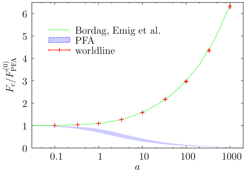
Figure 3: Casimir Force of a cylinder of radius $R=1$ above an infinite plate vs. the distance $a$. The force is normalized to the zeroth-order PFA formula. We observe an excellent agreement with the exact asymptotic solutions for small $a$ [44] and for large $a$ [43] up to $a=1000$.

The Casimir force for the sphere and cylinder is compared to the PFA estimates in Fig. 2 and 3 respectively. For similar comparisons for the Casimir energy, see [37]. We have normalized the force to the leading-order PFA, which is exact in the limit of vanishing separation $a$. The systematic study of the PFA, also from the worldline point of view, is summarized in Appendix A. We observe that the normalized force obtained with worldline numerics does not lie inside the range spanned by the ambiguity of the PFA estimates. Most prominently, the sign of the deviations from the $a\to 0$ limit is different in the Dirichlet scalar case, as can be understood in the worldline picture described above. These observations have been frequently made in the literature before [13, 53, 36, 42, 43].

In order to obtain Fig. 2 we have used ensembles with up to $n_{\mathrm{L}}=1.6\cdot 10^{6}$ and $N=2\cdot 10^{7}$. At very small distances $a$ the number of points per loop is not very important, since part of the systematic error is reduced by normalizing to the leading order result; thus, even $N=5000$ is sufficient for example for $a=0.0333$ at a precision level of $0.1\%$. On the other hand at $a=100$ the number of points per loop used was $1.5\cdot 10^{7}$. For larger distances the number of points per loop has to be increased far beyond $2\cdot 10^{7}$, since, as shown in Fig. 2. Even such high resolution is not sufficient to resolve the small sphere for larger distances.

Already anticipating our results for finite temperature, this observation gives us a rough estimate for the validity limits at small temperatures. Below, we observe that for $a/R\ll 1$ the maximum of the thermal contribution to the force density at low temperatures $T<1/R$ lies outside the sphere on scales $r\sim 1/T$. From the fact that ensembles with $N=1.5\cdot 10^{7}$ are reliable for those cases where the dominant contribution to the force density lies within $r\lesssim 100$, we conclude that temperatures above $T\gtrsim 0.01/R$ are accessible also in the limit $a\to 0$.

From an algorithmic point of view, the sphere-plate and cylinder-plate configurations differ with respect to computational efficiency also beyond the trivial dimensional factors: for a sphere at large separations, a large fraction of points of a worldline can be dropped right from the beginning, as they never see the sphere, i.e, they never lie on a ray inside the cone. The situation is different for a cylinder. Dealing with a two dimensional problem, we use two dimensional worldlines and the number of points per worldline which now have to lie in a wedge is higher than those lying in a cone for the sphere-plate case. Using comparable worldlines with a large number of points per loop, we thus expect the worldline numerics to break down at far larger distances $a$ than in the case of a sphere. This is indeed the case as is visible in Fig. 3.

For the Fig. 3 we have also used ensembles with up to $n_{\mathrm{L}}=1.1\cdot 10^{6}$ and $N=2\cdot 10^{7}$. At $a=100$, the number of points per loop used was $3\cdot 10^{6}$, and increased to $N=1\cdot 10^{7}$ for $a=333$ and up to $N=2\cdot 10^{7}$ for $a=1000$. As expected, the required number of points per loop for a certain $a$ is less here than in the case of a sphere. Even at such large separations as $a=1000$, we observe an excellent agreement with [43]. The corresponding estimate for the validity limits at small temperatures then is $T>0.001/R$.

IV Casimir effect at finite temperature

IV.1 General considerations

At finite temperature $T=1/\beta$, the free energy can be decomposed into its zero-temperature part $E_{\mathrm{c}}(0)$ and finite-temperature correction $\Delta E_{\mathrm{c}}(T)$,

$$E_{\mathrm{c}}(T)=E_{\mathrm{c}}(0)+\Delta E_{\mathrm{c}}(T).$$ (28)

The same relation holds for the Casimir force $F_{\mathrm{c}}(T)=F_{\mathrm{c}}(0)+\Delta F_{\mathrm{c}}(T)$.

Within the worldline representation of the free energy (II), the finite-temperature correction is purely driven by the worldlines with nonzero winding number $n$. Most importantly, the complicated geometry-dependent part of the calculation remains the same for zero or finite temperature.

Let us first perform a general analysis of the thermal correction for a generic Casimir configuration following an argument given in [8]. We start from the assumption that the Casimir free energy can be expanded in terms of the dimensionless product $aT$,

$$\frac{E_{\mathrm{c}}(T)}{E_{\mathrm{c}}(0)}=1+c_{1}aT+c_{2}(aT)^{2}+c_{3}(aT)^{3}+\dots$$ (29)

No negative exponents should be present in Eq. (29), since the thermal part of the energy disappears as $T\rightarrow 0$. Generically, the $T=0$ Casimir energy $E_{\mathrm{c}}(0)$ diverges for surfaces approaching contact $a\to 0$. From Eq. (29), we would naively expect the same for the thermal correction. If, however, sufficiently many of the first $c_{i}$’s in Eq. (29) vanish, then the thermal part of the Casimir energy is well behaved and without any divergence for $a\rightarrow 0$.

This turns out to be the case for two parallel plates ($c_{1}=c_{2}=0$, and $E_{\mathrm{c}}(0)\sim 1/a^{3}$) and for inclined plates ($c_{1}=0$, and $E_{\mathrm{c}}(0)\sim 1/a^{2}$) [31]. Consequently, an extreme simplification arises: the low-temperature limit of the thermal correction can be obtained by first taking the formal limit $a=0$. This was first observed in [8] and then successfully applied in [9].

In the following, we argue that there is no divergence in the local thermal force density in the limit $a\to 0$ for general geometries. For a generic geometry, the $a$-divergent part can only arise from the regions of contact as $a\rightarrow 0$. The divergence for these regions at $T=0$ is due to the diverging propertime integral over $1/\mathcal{T}^{1+D/2}$ which is bounded from below by $\sim a^{2}$. This is because for worldlines smaller than $a$ the worldline functional is always zero. At finite temperature the divergence in the thermal correction for $a\rightarrow 0$ is removed since one integrates now over $\exp(-n^{2}\beta^{2}/4\mathcal{T})/\mathcal{T}^{1+D/2}$, which is zero for every $n>0$ in the limit $\mathcal{T}\rightarrow 0$. The only nonanalyticity could arise from the infinite sum. That this is not the case can directly be verified: instead of integrating over the support $\mathcal{S}$, we integrate over $\mathcal{T}$ from zero to infinity, yielding

$$\sum_{n=1}^{\infty}\int_{0}^{\infty}\frac{\exp\left(\frac{-n^{2}\beta^{2}}{4\mathcal{T}}\right)}{\mathcal{T}^{1+D/2}}\,\mathrm{d}\mathcal{T}=(2T)^{D}\Gamma(D/2)\zeta(D).$$ (30)

For finite temperature $T>0$, Eq. (30) is a finite upper bound for the original local thermal force density. This procedure corresponds to substituting the critical regions of contact by broader (and infinitely extended) parallel plates, see [8]. The thermal contribution is estimated from above by flattening the surfaces in the contact region. The local thermal contribution to the Casimir force of the original configuration is clearly smaller than the finite thermal contribution of parallel plates. As the latter does not lead to divergences for $a\to 0$, there can also be no divergence for the general curved case arising from the contact regions. Of course, infinite geometries may still experience an infinite thermal force, as it is the case for two infinitely extended parallel plates, but the local thermal contribution to the force density will be finite. From a practical viewpoint, taking the limit $a\rightarrow 0$ first simplifies the calculations considerably.

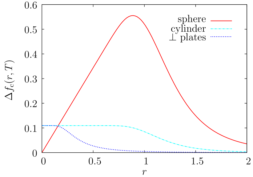
Figure 4: The (negative) thermal force density Eq. (IV.1) for perpendicular plates (dashed blue line), cylinder above plate (dotted dashed line) and sphere above plate (solid red line) both of radius $R=1$ in the zero-distance limit $a\to 0$ for $T=1$. The sphere-plate curve represents the radial density including the radial measure factor $\sim 2\pi r$. The thermal force densities of cylinder and perpendicular plates at $r=0$ are equal to the force density of two parallel plates, $\pi^{2}/90\approx 0.1097$. The thermal force density in the sphere-plate case has a maximum of $\approx 2\pi\times\pi^{2}/90$, where the factor $2\pi$ arises from the cylindrical measure. Note that a considerable fraction of the force density lies outside the sphere which only extends to $r=1$. As the temperature drops, the maximum moves monotonously to the right.

Another important feature of low-temperature contributions to the Casimir effect is the spread of the thermal force density over regions of size $\sim 1/T$ even for very small separations $a$. This phenomenon has first been demonstrated for the configuration of two perpendicular plates at a distance $a$ [8]. (In this configuration, the sphere in Fig. 1 is replaced by a vertical semi-infinite plate extending along the positive $z$ axis and an edge at $z=0$.) The thermal force density $\Delta f_{\mathrm{c}}(r,T)=f_{\mathrm{c}}(r,T)-f_{\mathrm{c}}(r,0)$ for this case as a function of the coordinate $r$ on the infinite surface measuring the distance from the edge (i.e., the contact point at $a=0$) can indeed be obtained analytically on the worldline from the thermal force,

$$\Delta F_{\mathrm{c}}(\beta)=-\frac{L_{y}}{16\pi^{2}}\sum_{n=1}^{\infty}\left\langle\int\mathrm{d}r\!\int_{r^{2}/\lambda_{1}^{2}}^{\infty}\frac{e^{-\frac{n^{2}\beta^{2}}{4\mathcal{T}}}}{\mathcal{T}^{3}}\,\mathrm{d}\mathcal{T}\right\rangle.$$ (31)

Here, $\lambda_{1}$ is a worldline parameter measuring the extent of half a unit worldline, i.e., the distance measured in $x$ direction from the left end to the center of mass. It is clear from Fig. 1 that the lower bound in the $\mathcal{T}$ integral in Eq. (31) is given by $r^{2}/\lambda_{1}^{2}$: this is the minimal scaling value for which the worldline intersects the semi-infinite vertical plate. From Eq. (31), we read off the following force density:

$$\frac{\Delta f_{\mathrm{c}}(r,T)}{L_{y}}= -\frac{\pi^{2}\,T^{4}}{90}$$

$$+\frac{1}{\pi^{2}}\!\sum_{n=1}^{\infty}\!\left\langle e^{-\frac{n^{2}\lambda_{1}^{2}}{4r^{2}T^{2}}}\Big{(}\frac{T^{4}}{n^{4}}+\frac{T^{2}\lambda_{1}^{2}}{4n^{2}r^{2}}\Big{)}\right\rangle,$$ (32)

Analytic results for the thermal force can be obtained by rescaling the radial coordinate $r\rightarrow\lambda_{1}r$ per worldline and using $\langle\lambda_{1}\rangle=\pi/2$. The thermal force between the perpendicular plates in the limit $a\to 0$ upon integration then yields $\Delta F_{\mathrm{c}}(T)=-\zeta(3)\,L_{y}T^{3}/4\pi$ in agreement with [5].

The perpendicular-plates configuration is special as it features a scale invariance in the $a\to 0$ limit: Eq. (IV.1) remains invariant under $T\rightarrow T\alpha,\ r\rightarrow r/\alpha$ and $\Delta\tilde{f}_{\mathrm{c}}\rightarrow\Delta\tilde{f}_{\mathrm{c}}/\alpha^{4}$ for arbitrary $\alpha$. As a consequence, knowing (IV.1) for a single temperature value, say $T=1/a$, is sufficient to infer its form for all other $T$. Equation (IV.1) is shown for $T=1/R,R=1$ in Fig. 4. For $r<1/T$, the force density stays nearly constant, corresponding to the first term in (IV.1). It rapidly approaches zero for $r>1/T$. From this, we draw the important conclusion that the region of constant force density in $r$ direction can be made arbitrarily large by choosing sufficiently low $T$.

Similar consequences arise for temperature effects in other geometries. We plot the thermal force densities for the sphere-plate and cylinder-plate configuration in Fig. 4. The thermal force density for a cylinder above a plate at $a=0$ has a shape similar to the one of two inclined plates, whereas the radial force density of a sphere above a plate exhibits a maximum due to the cylindric measure factor $r$, see Fig. 4. Although these force densities are not scale invariant due to the additional dimensionful scale $R$ (sphere radius), its maximum nevertheless moves away from the sphere as the temperature drops. We conclude that no local approximate tools such as the PFA will be able to predict the correct thermal force in particular at low temperatures. The fact that the force densities for sphere and cylinder are not scale invariant leads to different temperature behaviors for $T<1/R$ and $T>1/R$ even in the limit $a\rightarrow 0$.

IV.2 Sphere above a plate

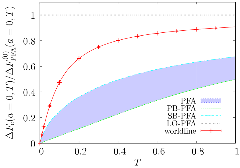
Figure 5: Thermal Casimir force of a sphere above a plate in the limit $a\to 0$ and for $R=1$. The worldline result and the PFA predictions are normalized to the leading-order PFA, cf. Eq. (36). The leading-order PFA predicts a $T^{3}$ behavior of the thermal force for all $T$. On the other hand, for small $T$ the plate-based PFA and the worldline result see a $T^{4}$ behavior, whereas the sphere-based PFA sees a $T^{4}\ln(T)$ one. For large $T\gg 1/R$ the behavior is $T^{3}$ for all curves. All predictions agree in the large $T$ limit. For very small $T$, the worldline result runs into the blue area which spans the PFA predictions.

Let us start with the expansion of the thermal force for $a\ll R$ and for small temperature $T\ll 1/R$. Following our general argument given above, no singularities in $a$ appears in the limit $a\to 0$. Also, we expect that the thermal force decreases with decreasing $R$. This motivates an expansion of the thermal force with only positive exponents for $a$ and $R$. Assuming integer exponents, dimensional analysis permits

$$\Delta F_{\mathrm{c}}(T) =c_{0}RT^{3}+c_{1}aT^{3}$$

$$+c_{2}R^{2}T^{4}+c_{3}aRT^{4}+\mathcal{O}\left({(a/R)^{2},(TR)^{5}}\right).$$ (33)

From our numerical results in the limit $a\to 0$, we observe a $T^{4}$ behavior of the thermal force, see Fig. 5. We conclude that $c_{0}\approx 0$ is negligible with respect to $c_{2}$ in the regime $T>0.01$ where numerical data is available. In fact, we conjecture that vanishes identically $c_{0}=0$; if so, also $c_{1}$ vanishes, since the configuration would otherwise be more sensitive to temperatures at small $a$ than at $a=0$. Our conjecture is supported by the following argument based on scaling properties: the dimensionless ratio of the thermal correction and zero-temperature force has to be invariant under the rescaling

$$a\rightarrow a/\alpha,\ \ \ R\rightarrow R/\alpha,\ \ \ T\rightarrow\alpha\,T.$$ (34)

The same holds for the ratio of $\Delta F_{c}(a,T)$ at $a=0$ and the zero-temperature force at $a\neq 0$. For $a\ll R$, we can use the PFA for the zero-temperature force, which to leading order yields $\sim R/a^{3}$. If $c_{0}\neq 0$, this leading ratio would be $\sim{c_{0}}(aT)^{3}$ which is invariant under the rescaling (34); in addition, this ratio would be invariant under (34) with $R$ fixed. If $c_{0}=0$, then this ratio is $\sim c_{2}Ra^{3}T^{4}$ which is invariant only under the full transformation (34).

The result that for $c_{0}\neq 0$ the thermal correction would exhibit the same $R$ dependence as the zero-temperature force for small distances $a\ll R$ is counterintuitive: whereas the radial force density in the small-distance limit at $T=0$ is peaked right under the sphere near $r\simeq 0$, the thermal correction arises from contributions at much larger $r$, cf. Fig. 4. As a simple estimate, we expect that the thermal correction is proportional to an effective area of the sphere, $\approx(a+R)2R+\pi R^{2}/2$, as seen by the worldlines. This estimate then is compatible with $c_{0}=c_{1}=0$ and $c_{2}/c_{3}\approx 1.8$.

The question arises why the PFA approximation yields a $T^{3}$ behavior despite the additional scale $R$. The reason is that $R$ appears only in the combination $r^{2}/R$ in the force density, such that $T\rightarrow\alpha T$, $r\rightarrow r/\alpha^{2}$ leaves the force density invariant up to a multiplicative constant.

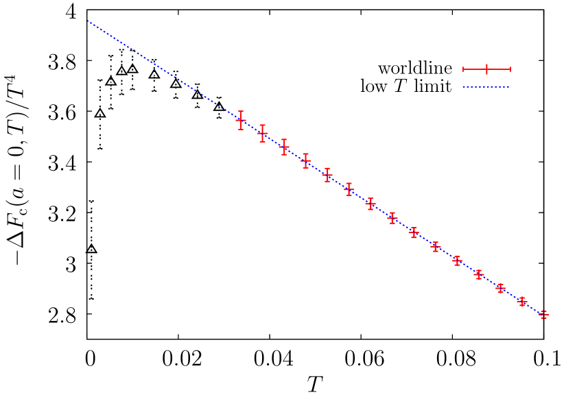
Figure 6: Low-temperature behavior of $-\Delta F_{\mathrm{c}}(T)/T^{4}$ for the sphere-plate configuration in the limit $a\to 0$ for $R=1$. For $0.03<T<0.1$, we observe a linear behavior which can be fitted to $\Delta F_{\mathrm{c}}(a=0,T)\approx-3.96\,R^{2}T^{4}+11.66\,R^{3}T^{5}$. We have used $40\,000$ loops with $2\cdot 10^{6}$ ppl each. For $T<0.03$, the number of points per loop used is not sufficient to resolve the sphere properly, inducing systematic errors (black triangles).

Let us return to Eq. (IV.2). For $c_{2}$ and $c_{3}$, we obtain numerically (see Figs. 6 and 7)

$$c_{2}\approx-3.96(5),\ \ \ c_{3}\approx-2.7(2).$$ (35)

These numbers can be confirmed by the exact $T$-matrix representation [54]. Note that both coefficients have the same sign, implying that the absolute value of the thermal correction to the Casimir force increases with increasing $a$ for sufficiently small $a$ and $T$. This apparently anomalous behavior can be understood in geometric terms within the worldline picture [19].

The system has a critical temperature $T_{\text{cr}}\simeq 0.34(1)/R$: For $T>T_{\text{cr}}$, the thermal force decreases monotonically for increasing sphere-plate separation $a$ in accordance with standard expectations. For smaller temperatures $T<T_{\text{cr}}$, the thermal force first increases for increasing separation, develops a maximum and then approaches zero as $a\rightarrow\infty$. The peak position is shifted to larger $a$ values for increasing thermal wavelength, i.e., decreasing temperature. In all cases, the force remains attractive, see Fig. 8. As an example, room temperature $T=300$K corresponds to the critical temperature for spheres of radius $R\simeq 2.6\mu$m. For larger spheres, room temperature is above the critical temperature such that the thermal force is monotonic. For smaller spheres, the thermal force is non-monotonic at room temperature. If, for instance, $T=70$K and $R=1.6\mu$m, the thermal force increases up to $a\simeq 9\mu$m.

The high-temperature limit $T\gg 1/R$ agrees with the PFA prediction for $a\to 0$ and reads

$$\Delta F_{\mathrm{c}}(T\rightarrow\infty)=-\frac{\zeta(3)R}{2}T^{3}.$$ (36)

In the limit $a\to 0$, the PFA yields Eq. (36) for all $T$. This is because geometrically the leading-order PFA corresponds to approximating the sphere by a paraboloid, which is a scale-invariant configuration at $a=0$. At finite $a$, the scale invariance is broken and a term $\sim+R\,\pi^{3}aT^{4}/45$ appears on the right-hand side of Eq. (36) at low temperature in the leading-order PFA. By contrast, we observe that the true $a\to 0$ limit is characterized by a $T^{4}$ behavior for small $T$ and $T^{3}$ behavior for large $T$. Also, the sign of the correction at finite $a$ is different: the full worldline result predicts an increase whereas the PFA correction reduces the absolute value of the force, see Fig. 7.

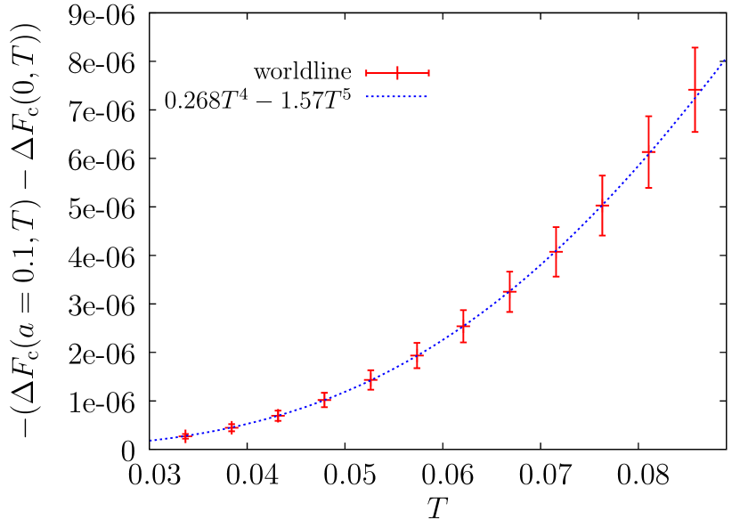
Figure 7: Plot of the $a$-dependent part of the (negative) thermal Casimir force for a sphere at $a=0.1$ and $R=1$ in the low-temperature regime. In the range $0.03<T<0.08$, the worldline data for $-(\Delta F_{\mathrm{c}}(0.1,T)-\Delta F_{\mathrm{c}}(0,T))$ is well approximated by $0.268\,T^{4}-1.57\,T^{5}$ (dashed blue curve), corresponding to a $c_{3}$ coefficient in Eq. (IV.2) $c_{3}\approx-2.7$. Note that the absolute value of the Casimir force has increased with $a$. We have used $40\,000$ loops with $2\cdot 10^{6}$ ppl each.

It is interesting to compare our results to another PFA scheme beyond the leading-order PFA: the plate based PFA. This scheme is not scale invariant at $a=0$, as the low-temperature limit for $a\ll R$ is also quartic and given by

$$\Delta F^{\mathrm{PFA}}_{\mathrm{PB}}(a\ll R,T\rightarrow 0)=-\frac{\pi^{2}T^{4}}{90}\,\pi R^{2}.$$ (37)

Equation (37), in fact, corresponds to the thermal force density of two parallel plates integrated over the area of the region below the sphere, $\pi R^{2}$. Numerically, the corresponding worldline coefficient is more than ten times larger than the PFA prefactor $\pi^{3}/90\approx 0.345$. In Eq. (37), the low-$T$ behavior at finite $a$ is exponentially suppressed, implying that the plate based PFA prediction for $c_{3}$ is zero – which is again in contradiction with our worldline analysis. The formulae (36) and (37) are derived in the Appendix. The thermal force at $a=0$ is shown together with the PFA predictions in Fig. 5.

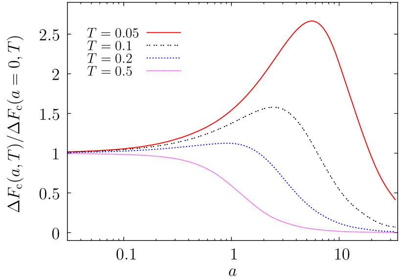
Figure 8: Thermal correction to the Casimir force of a sphere for various temperatures $T$ and $R=1$, normalized to the thermal force at $a=0$. For sufficiently small temperatures, the absolute value of the thermal force correction $\Delta F(T)$ first increases with increasing $a$. For $T\leq 0.05$ the small $a$ behavior is well described by $1+a(2.68RT^{4}-R^{2}15.7\,T^{5})/\Delta F(a=0,T)$. This verifies the fit used in Fig. 7 with coefficient linear in $\sim a$ in front of $T^{5}$. From this prediction, we would expect the curves to be monotonically decreasing for $T>2.7/15.7R\approx 0.17/R$ in the leading order. Due to higher-order terms, the $T=0.2$ curve still increases slightly first. The statistical errors of the worldline calculation are of the order of the thickness of the curves.

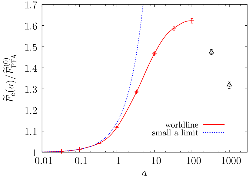
Figure 9: High-temperature coefficient $\widetilde{F}_{\mathrm{c}}(a)$ for the sphere-plate configuration normalized to the corresponding PFA coefficient. At large $a$, the normalized coefficient is conjectured to approach a constant. For small $a$, the behavior is well described by $1+(0.14\pm 0.015)\,a$. For $a>100$, systematic errors similar to those of Fig. 2 set in (black triangles); at finite temperature, these errors are even more pronounced due to a softer propertime exponent $5/2$.

We now turn to the high-temperature limit, in a strict sense corresponding to $T\gg 1/a$ and $T\gg 1/R$. The second requirement is automatically fulfilled in the small-distance limit $a\ll R$. Quantitatively, it turns out that the high-temperature regime is already approached for $T\gg 1/a$ and $T\ll 1/R$.

A special case arises for $a\to 0$, where the high-temperature limit agrees with the PFA prediction Eq. (36) in the leading order. For $a>0$, the high-temperature limit is linear in $T$ and the total force becomes classical, i.e., independent of $\hbar c$. This behavior is rather universal being a simple consequence of dimensional reduction in high-temperature field theories, or equivalently, of the linear high-temperature asymptotics of bosonic thermal fluctuations [55, 56, 57, 58, 59, 6]. In order to find the high-temperature limit, we perform the Poisson summation of the winding sum. The Poisson summation for an appropriate function $f$ reads

$$\sum_{n=-\infty}^{\infty}f(n/T)=\sqrt{2\pi}\,T\sum_{k=-\infty}^{\infty}\hat{f}(2\pi kT),$$ (38)

where $\hat{f}$ is the Fourier transform (including a $1/\sqrt{2\pi}$ prefactor) of $f$. Applying Eq. (38) to the winding sum, we obtain

$${2\sum_{n=1}^{\infty}}\exp\left(-\frac{n^{2}\beta^{2}}{4\mathcal{T}}\right)$$ (39)

$$=-1+2T\sqrt{\mathcal{T}\pi}+4T\sqrt{\mathcal{T}\pi}\sum_{k=1}^{\infty}\exp\left(-\mathcal{T}(2\pi kT)^{2}\right),$$

For finite $a$, the propertime integral is bounded from below and the last term is exponentially vanishing as $T\rightarrow\infty$. Evaluating the worldline integrals for the first two terms, we obtain

$$\Delta F_{\mathrm{c}}(a,T)=-F_{\mathrm{c}}(a)+T\widetilde{F}_{\mathrm{c}}(a).$$ (40)

The evaluation of $\widetilde{F}(a)$ is analogous to Eq. (18),

$$\widetilde{F}_{\mathrm{c}}(a)=-\frac{1}{8\sqrt{\pi}}\,\left\langle\int_{0}^{\infty}\mathrm{d}r\,r\int_{\mathcal{S}(r)}^{\infty}\frac{\mathrm{d}\mathcal{T}}{\mathcal{T}^{5/2}},\ \right\rangle.$$ (41)

where the support $\mathcal{S}(r)$ is the same as in the $T=0$ case, see Eqs. (17) and (18).

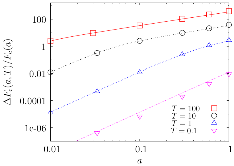
Figure 10: Thermal correction to the Casimir force for a sphere with $R=1$ normalized to the zero temperature force for various temperatures and $a<R$. The worldline results (symbols) should be compared with the PFA estimate (lines). We observe that this ratio of thermal to zero-temperature force is surprisingly well described by the PFA for a wide parameter range, especially in the high-temperature regime. This happens because both $\widetilde{F}_{\mathrm{c}}(a)$ and $F_{\mathrm{c}}(a)$ increase with respect to the PFA with roughly the same rate, see Fig. 2 and Fig. 9.

The Casimir force remains attractive also for high temperatures. The function $\widetilde{F}_{\mathrm{c}}(a)$, normalized to the PFA prediction

$$\widetilde{F}^{\mathrm{PFA}}_{\mathrm{c}}(a) =-\frac{R\,\zeta(3)}{8a^{2}},$$ (42)

is shown in Fig. 9. The function $a^{2}\widetilde{F}_{\mathrm{c}}(a)$ is monotonically increasing on $0<a<100$ (similar to $a^{3}F_{\mathrm{c}}(a)$). At small $a$, we obtain

$$\frac{\widetilde{F}_{\mathrm{c}}(a)}{\widetilde{F}^{\mathrm{PFA}}_{\mathrm{c}}(a)}=1+(0.14\pm 0.015)a.$$ (43)

In analogy to the zero-temperature force, we conjecture that also $a^{2}\widetilde{F}_{\mathrm{c}}(a)$ remains monotonically increasing and finally approaches a constant for $a\rightarrow\infty$. A consequence of this conjecture is that the high-temperature limit then has a simple form, $T\gg 1/a$, without any relation to $R$. Indeed, demanding

$${\Delta}F_{\mathrm{c}}(a,T)=-F_{\mathrm{c}}(a)+T\widetilde{F}_{\mathrm{c}}(a,T)<0$$ (44)

for a fixed $T$, the limit $a\rightarrow\infty$ corresponds immediately to $T\gg 1/a$, since $a^{3}F_{\mathrm{c}}(a)$ itself approaches a constant. Our numerical data shown in Fig. 9 is indeed compatible with this conjecture. However, the large-$a$ limit is difficult to assess due to the onset of systematic errors for $a>100$.

Comparing Fig. 2 and 9, we notice that the zero-temperature force $F_{\mathrm{c}}(a)$ and the high temperature coefficient $\widetilde{F}_{\mathrm{c}}(a)$ behave similarly. This is not surprising since $\widetilde{F}_{\mathrm{c}}(a)$ in $D=4$ Minkowski space corresponds to $F_{\mathrm{c}}(a)$ in $D=3$ Euclidean space due to dimensional reduction in the high-temperature limit. For finite $a$, the high-temperature limit is already well reached for $T\gtrsim 1/2a$. In the PFA approximation, the weaker thermal force at not too small temperatures is normalized by the weaker zero-temperature force, leading to an accidental cancellation, such that for $T\gtrsim 1/2a$

$$\frac{\Delta{\widetilde{F}_{\mathrm{c}}}(a)}{F_{\mathrm{c}}(a)}\,T\approx\frac{90\,\zeta(3)}{\pi^{3}}\,aT\approx 3.49\,aT,$$ (45)

independently of $R$. A comparison between the full worldline result and the PFA for the normalized force is shown in Fig. 10 for various $a$ and $T$. Since for small separations $a<R$, the PFA is a reasonable approximation already at medium temperature $1/2a>T>1/2R$, see Fig. 5, we observe that the ratio between thermal Casimir force and zero-temperature result is surprisingly well described by the PFA for quite a wide parameter range. We stress that the PFA is inapplicable for each quantity alone.

IV.3 Cylinder above a plate

Analogous to the sphere-plate case, we start with the expansion of the thermal force at low temperature $T$ and for $a\ll R$ as in Eq. (34). Again, we allow only for positive exponents for $a$ and $R$. Even though $\sqrt{R}$ terms appear in an $a/R\ll 1$ expansion at zero temperature, our numerical results at small finite temperatures, somewhat surprisingly, are consistent with an expansion of the type

$$\frac{\Delta F_{\mathrm{c}}(T)}{L_{y}}=c_{2}RT^{4}+c_{3}aT^{4}+\mathcal{O}\left(T^{9/2}\right).$$ (46)

The potential leading-order terms $c_{0}\sqrt{R}T^{7/2}$ and $c_{1}\sqrt{a}T^{7/2}$ are expected to be zero similar to the sphere-plate case, see above, since the configuration of a cylinder above a plate is not invariant unter $a\rightarrow a/\alpha$ and $T\rightarrow\alpha T$. We have no evidence for a term $\sim\sqrt{aR}T^{4}$, which would lead to a nonanalytic increase of the force. Thus at small temperatures, the powers of $T$ are found to be integers in leading order. Similar to the sphere-plate case, we expect the low-temperature contributions to the thermal force to be proportional to the effective area $\approx L_{y}(2R+a)$ seen by the distant worldlines. This results in the rough estimate $c_{2}/c_{3}\approx 2$, which also implies that both coefficients have the same sign.

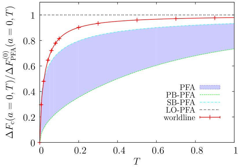
Figure 11: Normalized thermal contribution to the Casimir force of a cylinder above a plate for $R=1$ in the limit $a\to 0$. The worldline result and the PFA predictions are normalized to the leading-order PFA Eq. (48). The leading-order PFA predicts a $T^{7/2}$ behavior of the thermal force for all $T$. On the other hand, worldline numerical data is compatible with a $T^{4}$ behavior for small $T\ll 1/R$ and a $T^{3}$ behavior for large $T>1/R$. This is also observed in the plate-based PFA, whereas the cylinder based PFA goes as $T^{4}\ln(T)$ for small $T$. All predictions agree in the high-temperature limit. The worldline result enters the blue area for small $T$ into, which is the region spanned by the different PFA approximations.

In the limit $a\to 0$, our data in the regime $T>0.01$ is compatible with a $T^{4}$ behavior of the thermal force. For $c_{2}$ and $c_{3}$, we obtain (see Figs. 12 and 13)

$${c_{2}\approx-1.007(7),\ \ \ c_{3}\approx-0.41(4).}$$ (47)

As in the case of the sphere, both coefficients have the same sign, i.e., the absolute value of the thermal Casimir force increases with increasing $a$ for sufficiently small $a$ and $T<T_{\mathrm{cr}}$. For the critical temperature, we obtain $T_{\mathrm{cr}}\approx 0.31(1)/R$. As in the case of a sphere, the thermal force decreases monotonically with increasing $a$ for $T>T_{\mathrm{cr}}$; below the critical temperature, the thermal force first increases up to a maximum and then decreases again approaching zero for $a\rightarrow\infty$. The position of the maximum depends on $T$ and increases with inverse temperature, see Fig. 14. In both cases, however, the thermal force remains attractive.

The high-temperature limit $T\gg 1/R$ agrees with the PFA prediction in the limit $a\to 0$ as expected,

$$\frac{\Delta F_{\mathrm{c}}(T\rightarrow\infty)}{L_{y}}=\frac{3\,\zeta(1/2)\zeta(7/2)\sqrt{R}}{4\sqrt{2}\pi}T^{\frac{7}{2}}\approx-0.278\sqrt{R}T^{\frac{7}{2}}.$$ (48)

As for the sphere, the PFA predicts the same force law (48) in the limit $a\to 0$ for all $T$. At finite $a$, the scale invariance is broken and a term $\sim+0.185a\sqrt{R}T^{9/2}$ appears on the right-hand side of Eq. (48) in leading-order PFA at low temperature. By contrast, we observe different power laws for different temperatures in the limit $a\to 0$: a $T^{4}$ behavior for small $T$ and $T^{7/2}$ behavior for large $T$. Also, the sign of the finite-$a$ correction of the full result is opposite to that of the PFA, see Fig. 13, all of which is reminiscent to the sphere-plate case.

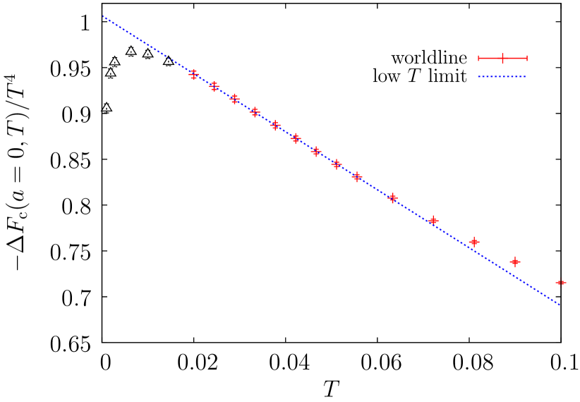
Figure 12: Low-temperature behavior of $-\Delta F_{\mathrm{c}}(T)/T^{4}$ for a cylinder above a plate for $R=1$ in the limit $a\to 0$. For $0.02<T<0.06$, we observe a linear behavior. In the range $0.03<T<0.05$, our data can be fitted to the form $\Delta F_{\mathrm{c}}(a=0,T)/L_{y}\approx-1.0065\,RT^{4}+3.163\,R^{2}T^{5}$. For $T<0.02$, systematic errors due to worldline discretization artifacts lead to a fast decrease of the data (black triangles). We have used $44\,000$ loops with $2\cdot 10^{6}$ ppl each.

Incidentally, the beyond-leading-order PFA schemes reflect the correct behavior much better. We observe that the cylinder-based PFA turns out to be the better approximation (as for the sphere-based PFA in the preceding section). This is opposite to the zero-temperature case. For the plate-based and cylinder-based PFA, we obtain

$$\frac{\Delta F^{\mathrm{PFA}}_{\mathrm{PB}}(0,T\rightarrow 0)}{L_{y}} =\frac{\pi^{2}T^{4}}{90}2R\approx-0.219\,RT^{4},$$ (49)

$$\frac{\Delta F^{\mathrm{PFA}}_{\mathrm{CB}}(0,T\rightarrow 0)}{L_{y}} =\frac{RT^{4}\left(3\pi^{4}+2\pi^{4}\ln\left(\frac{RT}{2\pi}\right)+180\zeta^{\prime}(4)\right)}{90\pi^{2}}$$

$$\approx(0.22\ln(RT/2\pi)+0.32)RT^{4}.$$ (50)

The plate-based result is equal to the thermal force of two parallel plates integrated over an area $2RL_{y}$. The plate-based coefficient is more than four times smaller than the worldline coefficient, whereas the leading coefficient of the cylinder-based formula becomes arbitrarily large as $T\rightarrow 0$. The formulae (49) and (50) are derived in the appendix. The thermal contribution to the force in the limit $a\to 0$ is shown together with the PFA predictions in Fig. 11.

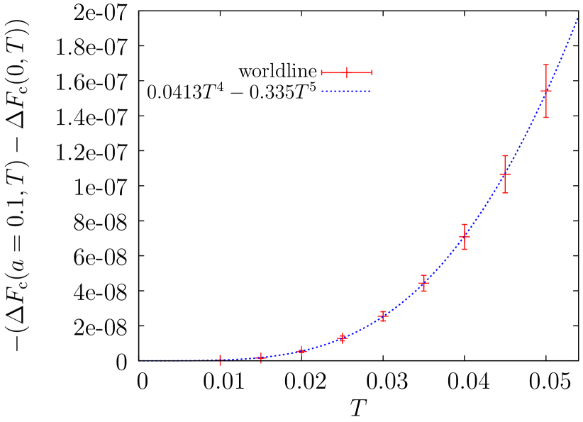
Figure 13: Plot of the $a$-dependent part of the (negative) thermal contribution to the Casimir force for the cylinder-plate configuration at $a=0.1$ and $R=1$ in the low-temperature regime. In the range $0.025<T<0.05$, the worldline data for $-(\Delta F_{\mathrm{c}}(0.1,T)-\Delta F_{\mathrm{c}}(0,T))$ is well approximated by $0.04125\,T^{4}-0.335187\,T^{5}$. We thus conclude that the $c_{3}$ coefficient in Eq. (46) is $\approx-0.4125$. Note that the absolute value of the Casimir force has increased with $a$. We have used $44\,000$ loops with $2\cdot 10^{6}$ ppl each.

Let us now investigate the high-temperature limit, which can be obtained by Poisson summation of the winding-number sum as in Eq. (39). A special case arises in the limit $a\to 0$, where the high-temperature limit corresponds to the PFA prediction Eq. (48) in leading order. For $a>0$, the high-temperature limit is again linear in $T$ and the total force “classical”, i.e., independent of $(\hbar c)$,

$$\Delta F_{\mathrm{c}}(a,T)=-F_{\mathrm{c}}(a)+T\widetilde{F}_{\mathrm{c}}(a)$$ (51)

as in Eq. (40), we obtain

$$\widetilde{F}_{\mathrm{c}}(a)=-\frac{L_{y}}{8\pi^{3/2}}\,\left\langle\int_{0}^{\infty}\mathrm{d}r\int_{\mathcal{S}(r)}^{\infty}\frac{\mathrm{d}\mathcal{T}}{\mathcal{T}^{5/2}}\right\rangle,$$ (52)

where the support $\mathcal{S}(r)$ is the same as in the $T=0$ case, see Eq. (27).

The Casimir force remains attractive also for high temperatures. The function $\widetilde{F}_{\mathrm{c}}(a)$, normalized to the PFA prediction

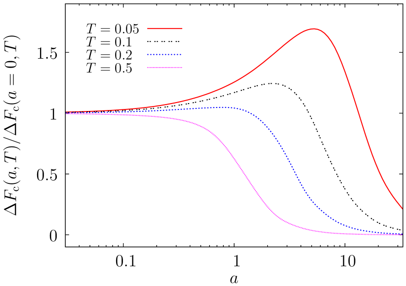
Figure 14: Thermal correction to the Casimir force of a cylinder above a plate for various temperatures $T$ and $R=1$ normalized to the thermal correction at $a=0$. For sufficiently small temperatures, the absolute value of the thermal force $\Delta F(T)$ first increases with increasing $a$. For $T\leq 0.05$, the small-$a$ behavior is well described by $a(0.4125T^{4}-3.35187\,RT^{5})/\Delta F(a=0,T)$. This verifies the fit found for Fig. 13 with a coefficient linear in $a$ in front of $T^{5}$. From this form, we would expect the curves to be monotonically decreasing for $T>0.41/3.35R\approx 0.12/R$ to leading order. Due to higher-order terms the $T=0.2$ curve still increases slightly at the beginning.

$$\widetilde{F}^{\mathrm{PFA}}_{\mathrm{c}}(a) =-\frac{3\sqrt{R}\,\zeta(3)}{32\sqrt{2}a^{5/2}},$$ (53)

is shown in Fig. 15. The function $a^{5/2}\widetilde{F}_{\mathrm{c}}(a)$ is monotonically increasing for $0<a<1000$ and is reminiscent to $a^{7/2}F_{\mathrm{c}}(a)$. At small $a$, we obtain

$$\frac{\widetilde{F}_{\mathrm{c}}(a)}{\widetilde{F}^{\mathrm{PFA}}_{\mathrm{c}}(a)}=1+(0.125\pm 0.017)a.$$ (54)

At large $a$, we find using Eq. (44) and the analytical zero-temperature law [43],

$$\frac{\widetilde{F}_{\mathrm{c}}(a)}{\widetilde{F}^{\mathrm{PFA}}_{\mathrm{c}}(a)}\simeq 1.46(2)\frac{a^{5/2}}{(a+R)^{2}\ln(a+R)}.$$ (55)

We can compare our results with those of an analytical result [43] in the limit $R\ll H=R+a$. The leading-order thermal contribution to the Casimir force in this computation based on scattering theory reads

$$\Delta F_{\mathrm{c}}(a,T)=L_{y}T\int_{0}^{\infty}\frac{qe^{-2q(R+a)}\ \text{st}(q)}{\ln(qR)}\,\mathrm{d}q,$$ (56)

where the integrand has been approximated to leading order in $\ln^{-1}(qR)$. Here, $\text{st}(q/T)$ is a $2\pi T$ periodic sawtooth function which in the range from $0$ to $2\pi T$ is given by $-q/(2\pi T)+1/2$. The authors of [43] have given a simple estimate of the integral for the limit $R\ll 1/2\pi T$ by replacing $\ln(qR)$ by $\ln(2\pi RT)$ and carrying out the resulting integral. We compare our worldline results with Eq. (56) as well as with the simple estimate in Fig. 16 and 17.

Here, we propose another estimate which is valid for arbitrary $T>1/(R+a)$. In this case, the sawtooth function is approximately constant for $q<1/(R+a)$. We approximate the logarithm by inserting the value $q_{0}$ for which $q\exp(-2q(R+a))$ is maximal: $q_{0}=1/2(R+a)$. In turn for $T<1/(R+a)$, the logarithm can be approximated by insertion of the value $q_{0}$ where $q\exp(-2q(R+a))\text{st}(q)$ has its first maximum: $q_{0}=\pi T/2$. We choose the first maximum, as the integrand is oscillating for $q>q_{0}$, such that cancellation can be expected to occur. However, choosing $q_{0}\sim T$ always leads to a regular $T^{4}/\ln(T)$ behavior for small $T$, whereas Eq. (56) changes sign at very small $T$, see Figs. 16 and 17. We thus conclude that Eq. (56) is valid for not too small $T$.

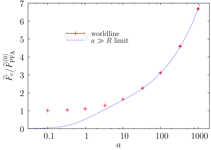
Figure 15: High-temperature coefficient $\widetilde{F}_{\mathrm{c}}(a)$ normalized to the corresponding PFA coefficient for a cylinder above a plate. The large-$a$ behavior is well described by Eq. (55). At small $a$, we find a behavior $\sim 1+(0.125\pm 0.017)a$.

The thermal contribution to the Casimir force then reads

$$\Delta F_{\mathrm{c}}(a,T)=\frac{-TL_{y}}{\ln(q_{0})}\frac{\mathrm{d}}{\mathrm{d}a}\frac{\text{coth}(2\pi(R+a)T)-\frac{1}{2\pi(R+a)T}}{8(R+a)},$$ (57)

where $q_{0}=2\pi RT$ in the Emig et al. approximation [43], whereas $q_{0}=R/2(a+R)$ for $T>1/(R+a)$ and $q_{0}=R\pi T/2$ for $T<1/(R+a)$ in the approximation proposed here. See Figs. 16 and 17 for the results at $a=10R$ and $a=100R$ respectively. In the small $T$ limit, Eq. (57) reads

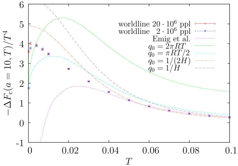
Figure 16: Thermal contribution to the Casimir force for a cylinder above a plate for $a=10$ and $R=1$ compared with the analytic result (56) (“Emig et al.” [43]) and various approximations as discussed in the text. Here, we use the abbreviation $H=R+a$. Remarkably, our proposed estimates using $q_{0}=\pi RT/2$ and $q_{0}=1/2H$, cf. Eq. (57), describe the actual behavior far better than the analytic result (56), which changes sign as $T\rightarrow 0$. Also the $T>1/(R+a)$ approximation using $q_{0}=1/2H$ remains a reasonable estimate even for $T<1/(R+a)$. For the worldline data, we have used $5000$ loops with $2\cdot 10^{7}$ ppl and $7000$ loops with $2\cdot 10^{6}$ ppl.

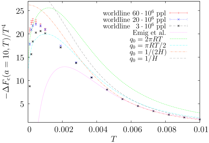
Figure 17: Thermal contribution to the Casimir force for a cylinder above a plate for $a=100$ and $R=1$ compared with the analytic result (56) (“Emig et al.” [43]) and various approximations as discussed in the text. Even at such large separations, we observe that the analytic result (56) becomes invalid and even changes sign as the temperature approaches zero. Incidentally our simple $T>1/(R+a)$ approximation using $q_{0}=1/2H$ describes the actual behavior rather well also for smaller temperatures. For the worldline data, we have used $2500$ loops with $6\cdot 10^{7}$, $5000$ loops with $3\cdot 10^{7}$ ppl and $14000$ loops with $3\cdot 10^{6}$ ppl.

$$\Delta F_{\mathrm{c}}(a,T)=L_{y}\frac{2\pi^{3}(a+R)T^{4}}{45\text{ln}(q_{0})}.$$ (58)

Writing this as $c(T,a,R)T^{4}$, the $T^{4}$ coefficient $c$ always disappears for $q_{0}\sim T$ as $T\rightarrow 0$. In our numerical worldline analysis, the systematic discretization errors lead to a vanishing of the corresponding coefficient as well, since the number of points per worldline becomes insufficient for resolution of the cylinder at very small $T$. For an increasing number of points per worldline, however, our data actually appears to point to a non-vanishing coefficient, see Figs. 16 and 17. In any case, we expect the leading-order multipole expansion which is behind the asymptotic result (56) to break down at low temperatures due to the geothermal interplay.

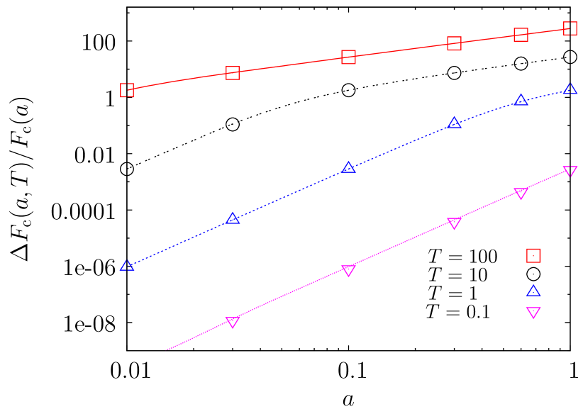
Figure 18: Thermal correction to the Casimir force for a cylinder with $R=1$ normalized to the zero-temperature force for various temperatures and $a<R$. The worldline results (symbols) are in a better agreement with the PFA estimates (lines) than in the case of a sphere, see Fig. 10. The normalized PFA results agree with the worldline results for not too low $T$ because again both $\widetilde{F}_{\mathrm{c}}(a)$ and $F_{\mathrm{c}}(a)$ increase with respect to the PFA with roughly the same rate, see Fig. 3 and Fig. 15.

For large $T$ on the other hand, Eq. (57) becomes

$$\Delta F_{\mathrm{c}}(a,T)=-\frac{L_{y}\left(1-T\pi(a+R)\right)}{8\pi\ln(q_{0})(R+a)^{3}}.$$ (59)

We observe that the negative of the $T$-independent part approaches the zero-temperature limit of the Casimir force for large $a/R$ faster if we choose $q_{0}=1/(R+a)$ rather than $q_{0}=1/2(R+a)$. This choice of $q_{0}=1/(R+a)$ then constitutes our second estimate for $T>1/(R+a)$.

For not too small $T$, the analytic result and the various $q_{0}$ approximations nicely agree with our worldline data, see Figs. 16 and 17. For higher temperature, the behavior becomes $\sim T$ and the different results acquire different slopes which partly disagree for $T\rightarrow\infty$. For $a=10$, the analytic result becomes $\sim 0.000424L_{y}T$, the $q_{0}=1/(R+a)$ approximation yields $\sim 0.000431L_{y}T$, and the $q_{0}=1/2(R+a)$ approximation $\sim 0.000334L_{y}T$. The numerical worldline result is $\sim 0.00041(3)L_{y}T$.

At $a=100$ and high $T$, the analytic result is $\sim 2.57\cdot 10^{-6}L_{y}T$, the $q_{0}=1/(R+a)$ approximation yields $\sim 2.66\cdot 10^{-6}L_{y}T$ and the $q_{0}=1/2(R+a)$ approximation $\sim 2.31\cdot 10^{-6}L_{y}T$. The worldline result is $\sim 2.4(9)\cdot 10^{-6}L_{y}T$.

For large $a+R$, the temperature coefficient becomes $0.125/(R+a)^{2}\ln(R+a)$ for both $q_{0}=1/(R+a)$ and $1/2(R+a)$. For the analytic result the corresponding prefactor is greater than $0.123$ and may become $0.125$ for $H\rightarrow\infty$. The corresponding worldline prefactor is $0.116(2)$, see Eq. (55).

Let us return to the high-temperature discussion, and finally remark that also in the case of a cylinder the thermal Casimir force normalized to the zero temperature result is well described by the PFA for $T\gtrsim 1/2a$. Analogously to Eq. (45), we conclude from the dimensional-reduction argument, that the ratio of thermal to zero-temperature force in the high-temperature limit $T\gtrsim 1/2a$ is approximately

$$\frac{\Delta{\widetilde{F}_{\mathrm{c}}}(a)}{F_{\mathrm{c}}(a)}\,T\approx\frac{72\,\zeta(3)}{\pi^{3}}\,aT\approx 2.79\,aT.$$ (60)

Also at medium temperatures this ratio is surprisingly well described by the PFA, even better than in the case of a sphere, see Fig. 10. The normalized thermal force is shown in Fig. 18 for various $a$ and $T$.

V Conclusions

In this work, we have analyzed the geometry-temperature interplay in the Casimir effect for the case of a sphere or a cylinder above a plate. Since finite-temperature contributions to the Casimir effect are induced by a thermal population of the fluctuation modes, the geometry has a decisive influence on the thermal corrections as the mode spectrum follows directly from the geometry. A strong geometry-temperature interplay can generically be expected whenever the length scale set by the thermal wavelength is comparable to typical geometry scales.

Within our comprehensive study of the Casimir effect induced by Dirichlet scalar fluctuations for the sphere-plate and cylinder-plate geometry, we observe several signatures of this geometry-temperature interplay: the thermal force density is delocalized at low temperatures. This is natural as only low-lying long-wavelength modes in the spectrum can be thermally excited at low $T$. As a consequence, the force density is spread over length scales set not only by the geometry scales but also by the thermal wavelength. This implies that local approximation techniques such as the PFA are generically inapplicable at low temperatures. Quantitatively, the low-temperature force follows a $T^{4}$ power law whereas the leading-order PFA correction predicts a $T^{3}$ behavior – a result which has often been used in the analysis of experimental data. Only for ratios of thermal to zero-temperature forces, we observe a potentially accidental agreement with the PFA prediction for larger temperatures. Here, the errors introduced by the PFA for the aspect of geometry appear to cancel, whereas the thermal aspects might be included sufficiently accurately.

Another signature of this geometry-temperature interplay is the occurrence of a non-monotonic behavior of the thermal contribution to the Casimir force. Below a critical temperature, this thermal force first grows for increasing distance and then approaches zero only for larger distances. This phenomenon is not related to a competition of polarization modes as in [20, 21], but exists already for the Dirichlet scalar case. The phenomenon can be understood within the worldline picture of the Casimir effect [19] being triggered by a reweighting of relevant fluctuations on the scale of the thermal wavelength. From this picture, it is clear that the phenomenon is not restricted to spheres or cylinders above a plate; we expect it to occur for general compact or semi-compact objects in front of surfaces, as long as the lateral surface extension is significantly larger than the thermal wavelength. In fact, another consequence of the delocalized force density is that edge effects due to finite plates or surfaces will be larger for the thermal part than for the zero-temperature force.

Our results have been derived for the case of a fluctuating scalar field obeying Dirichlet boundary conditions on the surfaces. For different fields or boundary conditions, the temperature dependence can significantly differ from the quantitative results found in this work. This is only natural as different boundary conditions can strongly modify the fluctuation spectrum. For instance, the thermal part of the free energy in the sphere-plate case exhibits different power laws for Dirichlet or Neumann boundary conditions in the low-temperature and small-distance limit [9]. For future realistic studies of thermal corrections, all aspects of geometry, temperature, material properties, boundary conditions and edge effects will have to be taken into account simultaneously, as their mutual interplay inhibits a naive factorization of these phenomena.

Appendix A The proximity-force approximation (PFA)

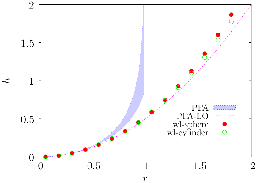
Figure 19: The effective heights predicted by the PFA for $a=0$, $R=1$ and $T=0$ compared with those of worldline numerics for a sphere and a cylinder, respectively, obtained from the $T=0$ force density. The PFA predictions lie in the blue area which is bounded by Eq. (64) from below and by Eq. (68) from above. The effective heights seen by worldlines are well approximated by the leading order PFA for $r$ not too large. We conclude that for small $a/R$ the force is described best by the leading order order PFA, since for small $a/R$ the force density is concentrated around $r=0$.

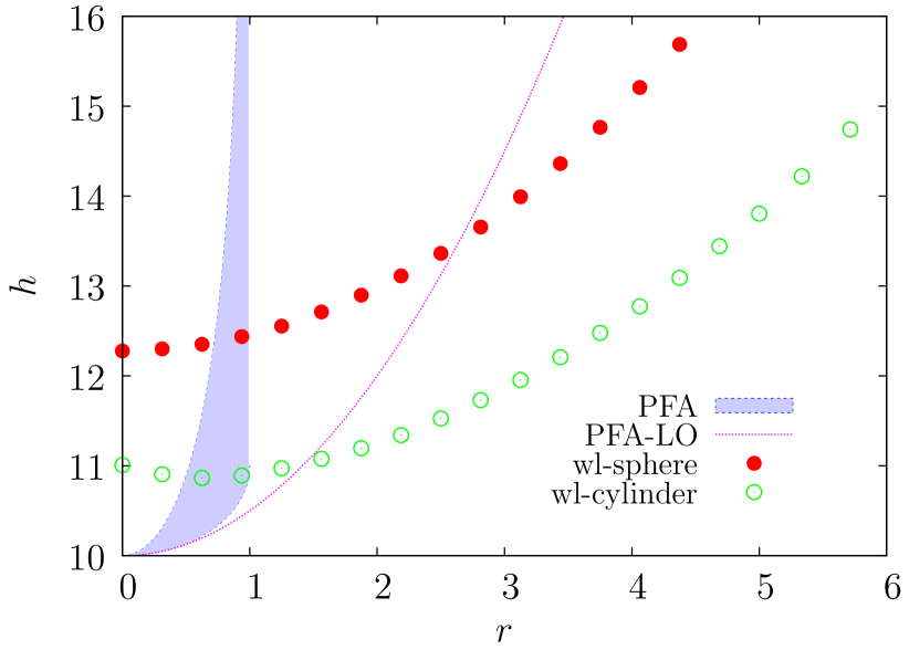
Figure 20: The effective heights predicted by the PFA for $a=10$, $R=1$ and $T=0$ compared with those of worldline numerics for a sphere and a cylinder, respectively, obtained from the $T=0$ force density. Note that the effective height for the cylinder is in a local maximum at $r=0$. At greater separations the heights seen by worldlines are on average lower than the PFA predictions resulting in greater Casimir force. Also at larger separations the leading order PFA reflects best the actual situation, while the ’sphere/cylinder based’ PFA turns out to be the worst.

The proximity force approximation is a scheme for estimating Casimir energies between two objects. In this approach, the surfaces of the bodies are treated as a superposition of infinitesimal parallel plates, and the Casimir energy is approximated by

$$E^{\mathrm{PFA}}(a)=\int_{\Sigma}\varepsilon^{\mathrm{PP}}(h)\,\mathrm{d}\sigma.$$ (61)

Here, one integrates over an auxiliary surface $\Sigma$, which should be chosen appropriately. The quantity $\varepsilon^{\mathrm{PP}}(h)$ denotes the energy per unit area of two parallel plates at a distance $h$ apart, which at zero temperature reads

$$\varepsilon^{\mathrm{PP}}(h)=-\frac{c_{\mathrm{PP}}}{h^{3}},$$ (62)

where $c_{\mathrm{PP}}=\pi^{2}/1440$ for the Dirichlet scalar case.

As the PFA does not make any reference to boundary conditions, all the formulas in this appendix are analogously valid for the electromagnetic case; all force formulas then have to be multiplied by a factor of two for the two polarization modes.

At finite temperature, the corresponding expression is

$$\frac{\Delta\varepsilon^{\mathrm{PP}}(h)}{c_{\mathrm{PP}}} =$$ (63)

$$\!\!\!\!\!\!\!\!\!\!\!\!\!\!\!\!\!\!\!\!\!\!\!\frac{1}{h^{3}}-\frac{90T}{h^{2}}\sum_{n=1}^{\infty}\frac{\coth(2n\pi hT)+2n\pi hT\text{csch}^{2}(2n\pi hT)}{\pi^{3}n^{3}}.$$

The distance is conventionally measured along the normal to $\Sigma$. The two extreme cases in which $\Sigma$ coincides with one of the two bodies provides us with a region spanning the inherently ambiguous estimates of the PFA.

For a sphere at a distance $a$ above a plate, we thus integrate either over the plate (’plate based’ PFA), or over the sphere (’sphere based’ PFA). The Casimir force is then obtained by taking the derivative of (61) with respect to $a$. However, for the ’sphere based’ PFA, $\mathrm{d}h/\mathrm{d}a\neq 1$ (see below). This implies that deriving the force estimate from the PFA of the energy in general is not the same as setting up the PFA directly for the force (the latter would correspond to a surface integral over the parallel-plates force per unit area). In this work, we use the derivation via the energy (61).

The dependence of the PFA prediction on the choice of $\Sigma$ disappears in the limit $a\rightarrow 0$ at zero temperature to leading order. This result shall be called ’leading-order’ PFA. It can also be obtained by expanding the surface of the sphere/cylinder to second order from the point of minimal distance to the plate and then using the ’plate based’ PFA for this expansion.

The corresponding expressions for $h$ read

$$h_{\mathrm{PB}} =a+R-\sqrt{R^{2}-r^{2}},$$ (64)

$$h_{\mathrm{SB}}=h_{\mathrm{CB}} =\frac{a+R}{\cos(\theta)}-R,$$ (65)

$$h_{\mathrm{LO}} =a+\frac{r^{2}}{2R}.$$ (66)

For $h_{\mathrm{PB}}$, we integrate over $[-R,R]$, for $h_{\mathrm{LO}}$ over all $r$ and for $h_{\mathrm{SB}}$, $h_{\mathrm{CB}}$ over $[-\pi/2,\pi/2]$ with an appropriate measure. Note that right underneath the sphere/cylinder all $h$ are equal to $a$. Demanding $\mathrm{d}\theta=\mathrm{d}r$ for $\theta\rightarrow 0$ we can transform the integration over $\theta$ into an integration over $r$ in a simple way by the substituting $\sin(\theta)\rightarrow r/R$. The integral then goes from $-R$ to $R$, and the corresponding $h$ reads

$$h_{\mathrm{SB}}=h_{\mathrm{CB}} =-R+R\frac{a+R}{\sqrt{R^{2}-r^{2}}}.$$ (67)

Also a measure factor resulting from $R\mathrm{d}\theta=R/\sqrt{R^{2}-r^{2}}$ and $\mathrm{d}h/\mathrm{d}a$ have to be taken into account. At zero temperature, we can absorb these factors into the new effective height

$$h_{\mathrm{SB-eff}}=h_{\mathrm{CB-eff}} =\frac{\sqrt{R}\left(a+R-\sqrt{R^{2}-r^{2}}\right)}{\left(R^{2}-r^{2}\right)^{1/4}}.$$ (68)

With or without the prefactors $h_{\mathrm{SB/CB}}$ is always greater than $h_{\mathrm{PB}}$ and $h_{\mathrm{LO}}$ and diverges for $r\rightarrow R$. Since the factor approaches $1$ for small $r$, all functions $h$ coincide in this limit.

The PFA can also be developed within worldline formalism. Calculating the Casimir force density for two parallel plates, we have to determine that value of propertimes $\mathcal{T}$ for which one dimensional worldlines, attached to one of the plates, touch the other plate for the first time. This event is encoded in the lower bound of the proper time integral, whereas the upper bound is set to infinity. Thus, we obtain

$$f_{\mathrm{c}}^{\mathrm{PP}}(h,\beta)=-\frac{1}{32\pi^{2}}\left\langle\int_{(h/\lambda)^{2}}^{\infty}\sum_{n=-\infty}^{\infty}\frac{e^{-\frac{n^{2}\beta^{2}}{4\mathcal{T}}}}{\mathcal{T}^{3}}\mathrm{d}\mathcal{T}\right\rangle.$$ (69)

The representation (69) is suitable for zero and low temperatures, whereas for high temperatures one should use in (69) the Poisson resummed winding sum (39). We encounter cumulants of worldline extents $\lambda$ in low and high temperature limits which can be determined via the analytic expression [37]

$$\left\langle\lambda^{D}\right\rangle=D(D-1)\Gamma(D/2)\zeta(D).$$ (70)

Let us now point out the difference between the PFA and the worldline approach. In the PFA, we always use one dimensional worldlines to determine the distance, whereas the worldline dimension in the full formalism corresponds to the dimension of the geometry. To obtain the Casimir force for configurations containing one infinite plate in the worldline formalism, we integrate over this infinite plate as in the plate-based approach. However, the integration does not stop at the end of the second body, which in the present case is a sphere or cylinder. At arbitrary large distances, there are still worldlines which see the sphere/cylinder, i.e., we have to integrate to infinity. We therefore expect the leading-order PFA to reflect best the exact force laws. However, the propertime support is not the same, and thus worldlines see an effective height different from the one of the leading-order PFA, see Fig. 19 and 20.

The shape of the effective worldline height is roughly the same for zero and high temperatures. But at low temperature, the worldlines are reweighted. Only worldlines for large propertimes contribute considerably and thus worldlines at larger distances from the sphere become increasingly more important. Also their inner structure comes into play. Using the ’plate based’ PFA, we ignore these effects and take into account only the region below the sphere/cylinder with the same function $h_{\mathrm{PB}}$ ; hence, the result is expected to be too small.

In the following, we apply Eq. (69) (multiplied by $\mathrm{d}h/\mathrm{d}a$ if necessary) to find the PFA expressions for the sphere and cylinder above an infinite plate, respectively.

A.1 Sphere above a plate

A.1.1 Leading-order PFA

For the sphere, the evaluation of the leading-order PFA results in an especially simple expression,

$$-\frac{\mathrm{d}}{\mathrm{d}a}E^{\mathrm{PFA}}_{\mathrm{LO}} =2\pi\,c_{\mathrm{PP}}\frac{\mathrm{d}}{\mathrm{d}a}\int_{0}^{\infty}\frac{r\,\mathrm{d}r}{\left(a+r^{2}/2R\right)^{3}}$$ (71)

$$=2\pi R\,c_{\mathrm{PP}}\frac{\mathrm{d}}{\mathrm{d}a}\int_{a}^{\infty}\frac{\mathrm{d}h_{\mathrm{LO}}}{h_{\mathrm{LO}}^{3}}=2\pi R\,\varepsilon^{\mathrm{PP}}(a).$$

Obviously, the relation $F^{\mathrm{PFA}}_{\mathrm{LO}}=2\pi R\,\varepsilon^{\mathrm{PP}}(a)$ remains valid also at finite temperature. We thus obtain

$$F^{\mathrm{PFA}}_{\mathrm{LO}}(a,T=0)=-\frac{2\pi R\,c_{\mathrm{PP}}}{a^{3}}=-\frac{\pi^{3}R\,}{720a^{3}}.$$ (72)

At finite $T$ and small $aT$ ($aT\lessapprox 1/2$), Eq. (69) yields

$$\Delta F^{\mathrm{PFA}}_{\mathrm{LO}}(a,T)=-\frac{R\,\zeta(3)}{2}T^{3}+\frac{aR\,\pi^{3}}{45}T^{4}.$$ (73)

For large $aT$ ($aT\gtrapprox 1/2$), the expression (63) leads directly to

$$\Delta F^{\mathrm{PFA}}_{\mathrm{LO}}(a,T) =\frac{\pi^{3}R\,}{720a^{3}}-\frac{R\,\zeta(3)}{8a^{2}}T$$ (74)

$$=-F^{\mathrm{PFA}}_{\mathrm{LO}}(a,0)+T\widetilde{F}^{\mathrm{PFA}}_{\mathrm{LO}}(a).$$ (75)

Note that at $a=0$ the leading-order PFA predicts a $T^{3}$ behavior of the thermal force for all $T$. At finite $a$, the validity of the low-temperature limit is independent of $R$. With increasing $a$ the absolute value of the PFA thermal force is always reduced, irrespective of $T$, quite the contrary to the full worldline results as discussed in the main text.

A.1.2 Plate-based PFA

Using Eq. (69), we obtain

$$-\Delta F^{\mathrm{PFA}}_{\mathrm{PB}}(a,T) =\frac{1}{8\pi}\int_{0}^{R}r\,\mathrm{d}r\left\langle\sum_{n=1}^{\infty}\int_{h_{\mathrm{PB}}^{2}/\lambda^{2}}^{\infty}\frac{e^{-\frac{\beta^{2}n^{2}}{4\mathcal{T}}}}{\mathcal{T}^{3}}\,\mathrm{d}\mathcal{T}\right\rangle=\frac{\zeta(4)R^{2}}{\pi\beta^{4}}+$$ (76)

$$\!\!\!\!\!\!\!\!\!\!\!\!\!\!\!\!\!\!\!\!\!\!\!\!\!\!\!\!\!\!\!\!\!\!\!\!\!\frac{1}{\pi}\sum_{n=1}^{\infty}\left\langle\frac{ae^{-\frac{n^{2}\beta^{2}\lambda^{2}}{4a^{2}}}(a+2R)}{n^{4}\beta^{4}}-\frac{e^{-\frac{n^{2}\beta^{2}\lambda^{2}}{4(a+R)^{2}}}(a+R)^{2}}{n^{4}\beta^{4}}-\frac{\sqrt{\pi}(a+R)\lambda\text{Erfc}\left(\frac{n\beta\lambda}{2a}\right)}{2n^{3}\beta^{3}}+\frac{\sqrt{\pi}(a+R)\lambda\text{Erfc}\left(\frac{n\beta\lambda}{2(a+R)}\right)}{2n^{3}\beta^{3}}\right\rangle.$$

Let us first analyze Eq. (76) for $a=0$,

$$\Delta F^{\mathrm{PFA}}_{\mathrm{PB}}(a=0,T) =-\frac{\zeta(4)R^{2}}{\pi}T^{4}+$$ (77)

$$\!\!\!\!\!\!\!\!\!\!\!\!\!\!\!\!\!\!\!\!\!\!\!\!\!\!\!\!\!\!\!\!\!\!\!\!\!\!\!\!\!\!\frac{1}{\pi}\sum_{n=1}^{\infty}\left\langle\frac{e^{-\frac{n^{2}\lambda^{2}}{4T^{2}R^{2}}}R^{2}}{n^{4}}T^{4}-\frac{\sqrt{\pi}R\lambda\text{Erfc}\left(\frac{n\lambda}{2TR}\right)}{2n^{3}}T^{3}\right\rangle.$$

Equation (77) distinguishes low- ($T{\ll}1/R$) and high-temperature ($T{\gg}1/R$) regimes. The low-temperature regime is already well approached for $T\lessapprox 1/2R$. For higher $T$, the thermal force is in the high-temperature regime, $T\gtrapprox 1/2R$.

At low temperatures, we have a $T^{4}$ behavior which is given by the first term in Eq. (77). For higher $T$, this $T^{4}$ term is canceled by the $T^{4}$ term with the exponential function, such that the leading behavior is given by the $T^{3}$ term. Then, expanding Eq. (77), we get a $T^{2}$ contribution:

$$\Delta F^{\mathrm{PFA}}_{\mathrm{PB}}(a=0,T) =-\frac{\zeta(3)R}{2}T^{3}+\frac{\zeta(2)}{4\pi}\left\langle\lambda^{2}\right\rangle T^{2}$$

$$=-\frac{\zeta(3)R}{2}T^{3}+\frac{\zeta(2)\zeta(2)}{2\pi}T^{2}.$$ (78)

Subtracting Eq. (78) from Eq. (77) and performing the Poisson resummation, we obtain the full $T{\gtrapprox}1/2R$ behavior at $a=0$

$$\Delta F^{\mathrm{PFA}}_{\mathrm{PB}}(0,T)=-\frac{\zeta(3)RT^{3}}{2} +\frac{\pi^{3}T^{2}}{72}$$

$$-\frac{\zeta(3)T}{8R}+\frac{\pi^{3}}{1440R^{2}}.$$ (79)

Thus, the leading large-$T$ behavior at $a=0$ is $\sim T^{3}$.

Let us now consider the case $a\neq 0$. For $a\ll R$ and low temperature ${T\lessapprox 1/2(R+a)\approx 1/2R}$, we have a $T^{4}$ behavior given by the first term in Eq. (76). The dependence on $a$ is exponentially suppressed. This corresponds to the case of two parallel plates with an area of $\pi R^{2}$, where the dependence on $a$ is suppressed exponentially as well.

At medium temperature, ${2(R+a)}\approx{2}R\gtrapprox{1/T}\gtrapprox{2}a$ only the second and third term in Eq. (76) are exponentially suppressed and can be neglected. The leading order can be found by expanding the remainder and considering only the converging sums.

To find the subleading terms, we again perform the Poisson resummation. For medium temperature ${2}R\gtrapprox{1/T}\gtrapprox{2}a$ and $a\ll R$, we then obtain

$$\Delta F^{\mathrm{PFA}}_{\mathrm{PB}}(a,T) =\frac{a(a+2R)\pi^{3}T^{4}}{90}-\frac{(a+R)\zeta(3)T^{3}}{2}$$ (80)

$$+\frac{\pi^{3}T^{2}}{72}-\frac{\zeta(3)}{8(a+R)}T+\frac{\pi^{3}}{1440(a+R)^{2}}.$$

The high-temperature limit for ${1/T}\lessapprox{2}a$ can be performed irrespective of the actual value $a/R$ by summing up the whole Eq. (76). The result reads

$$\Delta F^{\mathrm{PFA}}_{\mathrm{PB}}(a,T) =\frac{\pi^{3}R^{2}(3a+2R)}{1440a^{3}(a+R)^{2}}-\frac{R^{2}\text{ }\zeta(3)}{8a^{2}(a+R)}T$$ (81)

$$=-F^{\mathrm{PFA}}_{\mathrm{PB}}(a,0)+T\widetilde{F}^{\mathrm{PFA}}_{\mathrm{PB}}(a).$$ (82)

Note that Eq. (81) reduces to Eq. (74) for $a\rightarrow 0$ as it should.

For $a$ larger than $a\approx R$, the following temperature behavior occurs. At low temperature ${1/T}\gtrapprox{2}(R+a)$, a $T^{4}$ behavior arises from the first term in Eq. (76). At higher temperatures, the behavior becomes rapidly linear as given by Eq. (80), being valid for ${1/T}\lessapprox{2}a$.

The plate-based force can be obtained in closed form from Eq. (63) also without using the worldline language:

$$\Delta F^{\mathrm{PFA}}_{\mathrm{PB}}(a,T) =\frac{\pi^{3}R^{2}(3a+2R)}{1440a^{3}(a+R)^{2}}$$

$$-\frac{T}{8}\sum_{n=1}^{\infty}\Big{[}\frac{\text{coth}(2n\pi(a+R)T)}{(a+R)n^{3}}+\frac{\text{csch}^{2}(2an\pi T)\left[2an\pi RT+\left(R-(a+R)/2\right)\text{sinh}(4an\pi T)\right]}{a^{2}n^{3}}\Big{]}.$$ (83)

A.1.3 Sphere-based PFA

For the sphere-based PFA, the thermal Casimir force is given by

$$\Delta F_{\mathrm{SB}}^{\mathrm{PFA}}(a,T)=-\left\langle\frac{R^{2}}{8\pi}\int_{0}^{\pi/2}\sin(\theta)h_{\mathrm{SB}}^{\prime}(a)\mathrm{d}\theta\int_{h_{\mathrm{SB}}^{2}/\lambda^{2}}^{\infty}\sum_{n=1}^{\infty}\frac{e^{-\frac{n^{2}\beta^{2}}{4\mathcal{T}}}}{\mathcal{T}^{3}}\,\,\mathrm{d}\mathcal{T}\right\rangle,$$ (84)

where $h_{\mathrm{SB}}(a)$ is given by (65). For $a=0$, we obtain the PFA approximation using the worldline language

$$\Delta F_{\mathrm{SB}}^{\mathrm{PFA}}(a=0,T)= \left\langle\frac{2R^{2}\text{ln}\left(\frac{2RT}{n\lambda}\right)}{n^{4}\pi}T^{4}-\frac{\gamma R^{2}\zeta(4)}{\pi}T^{4}+\frac{R\zeta(3)}{2}T^{3}\right.$$

$$\left.-\sum_{n=1}^{\infty}\frac{R^{2}T^{4}}{4n^{4}\pi}\left(4+\frac{n^{2}\lambda^{2}}{R^{2}T^{2}}\right)\exp\left(-\frac{n^{2}\lambda^{2}}{4T^{2}R^{2}}\right)\left(\pi\text{Erfi}\left(\frac{n\lambda}{2RT}\right)-\text{Ei}\left(\frac{n^{2}\lambda^{2}}{4R^{2}T^{2}}\right)\right)\right\rangle,$$ (85)

where $\gamma$ is Euler’s constant. The expansion in $T$ does not terminate after a few terms, so we concentrate on the two leading coefficients. The coefficient in front of $T^{4}$ contains the worldline average $\langle\ln\lambda\rangle$. For an analytical expression, we note that $\ln\lambda=m\ln\lambda^{1/m}$. For large $m$, we get $\lambda^{1/m}\rightarrow 1$, such that we can expand the logarithm,

$$\langle\ln\lambda\rangle=\langle\lim_{m\rightarrow\infty}m(\lambda^{1/m}-1)\rangle=-1-\gamma/2+\ln(2\pi),$$ (86)

where we have used Eq. (70). Thus, the small-$T$ limit of Eq. (A.1.3) reads

$$\Delta F_{\mathrm{SB}}^{\mathrm{PFA}}(0,T) =\frac{R^{2}(2\zeta^{\prime}(4)+\zeta(4)(3+2\ln\left(\frac{RT}{\pi}\right)))}{\pi}T^{4}$$

$$-R^{3}\zeta(5)T^{5}.$$ (87)

At $a=0$, the PFA estimate $|\Delta F_{\mathrm{SB}}^{\mathrm{PFA}}(a=0,T)|$ lies above $|\Delta F_{\mathrm{PB}}^{\mathrm{PFA}}(a=0,T)|$, see Fig. 5. For not too small $T$, the worldline result lies above both these PFA predictions, but due to the logarithm in the $T^{4}$ coefficient the sphere-based PFA becomes larger at smaller $T$, such that the worldline force enters the area spanned by the PFA prediction, see Fig. 5.

The high-temperature limit can be obtained by expanding Eq. (A.1.3) about $T=\infty$. The converging terms give the leading-order behavior. For the subleading orders, one has to perform the Poisson summation, however, the integral involved is rather complicated and may still be inflicted with artificial convergence problems. The leading-order behavior for $a=0$ and large $T$ reads

$$\Delta F_{\mathrm{SB}}^{\mathrm{PFA}}(0,T) =-\frac{R\zeta(3)}{2}T^{3}+\frac{\pi^{3}}{72}T^{2}+\mathcal{O}(T),$$ (88)

and corresponds to the leading behavior of the plate-based limit (79).

Let us turn to the case of finite $a$. Expanding Eq. (84), we obtain the $a$ dependent part of the thermal force,

$$\Delta F_{\mathrm{SB}}^{\mathrm{PFA}}(a,T)- \Delta F_{\mathrm{SP}}^{\mathrm{PFA}}(0,T)=\frac{2aR\zeta(4)T^{4}}{\pi}\times$$

$$\left(1-\frac{a}{2R}+\frac{a^{2}}{3R^{2}}-\frac{a^{3}}{4R^{3}}+\dots\right)$$ (89)

The series has a form of $(R/a)\ln(1+a/R)$, which we verified explicitly to 10th order. Assuming that this form holds to all orders, we get

$$\Delta F_{\mathrm{SB}}^{\mathrm{PFA}}(a,T)-\Delta F_{\mathrm{SP}}^{\mathrm{PFA}}(0,T) =\frac{R^{2}\pi^{3}T^{4}}{45}\ln\left(1+\frac{a}{R}\right)$$ (90)

Note that the first two terms agree with the $T^{4}$ coefficient of the plate-based formula (80); we also see that the absolute value of the thermal force decreases with increasing $a$. As Eq. (90) was obtained by interchanging summation and integration, we cannot expect Eq. (90) to describe the full $a$ dependence for all $a$ and $T$. Indeed at $a$ fixed, the thermal correction $\Delta F_{\mathrm{SB}}^{\mathrm{PFA}}(a,T)$ becomes $\sim T$ as $T\rightarrow\infty$, which is clearly not the case for Eq. (90).

We can estimate the range of applicability of Eq. (90) as follows. At high temperature and $a\approx 0$, all PFA estimates agree. For large $T$, the leading behavior is $\sim T^{3}$, see e.g. Eq. (88). With increasing $a$ the force is still attractive. Demanding $\Delta F_{\mathrm{SB}}^{\mathrm{PFA}}(a,T)<0$ we see that that Eq. (90) leads to a positive thermal force for $a\gtrsim 1/T$. On the other hand in the low-temperature regime, the $a=0$ contribution is given by Eq. (A.1.3). Taking only the leading contribution into account and demanding $\Delta F_{\mathrm{SB}}^{\mathrm{PFA}}(a,T)<0$, we again obtain that the force becomes positive at $a\gtrsim 1/T$. These rather rough estimates demonstrate that the validity range for $a$ becomes narrower with increasing temperature. For very small $a$, however the thermal correction is linear in $a$ irrespectively of $T$, whereas the dependence on $a$ in the plate-based PFA is exponentially suppressed for small $T\ll 1/(R+a)$.

At large temperatures $T>1/a$, we have the familiar situation

$$\Delta F^{\mathrm{PFA}}_{\mathrm{SB}}(a,T)=-F^{\mathrm{PFA}}_{\mathrm{SB}}(a,0)+T\widetilde{F}^{\mathrm{PFA}}_{\mathrm{SB}}(a),$$ (91)

where

$$F^{\mathrm{PFA}}_{\mathrm{SB}}(a,0)=-\frac{\pi^{3}\left(6a^{2}-3aR+2R^{2}\right)}{1440a^{3}R}-\frac{\pi^{3}\ln\left(\frac{a}{a+R}\right)}{240R^{2}},$$ (92)

and

$$\widetilde{F}^{\mathrm{PFA}}_{\mathrm{SB}}(a)=\frac{(R-2a)\zeta(3)}{8a^{2}}-\frac{\ln\left(\frac{a}{a+R}\right)\zeta(3)}{4R}.$$ (93)

A.2 Cylinder above a plate

A.2.1 Leading order PFA

Unfortunately, a simple relation similar to $F^{\mathrm{PFA}}_{\mathrm{LO}}=2\pi R\,\varepsilon^{\mathrm{PP}}(a)$ does not hold any longer for the cylinder, such that the resulting formulas are not related to the known results of parallel plates and are rather complicated. For arbitrary $a$ and $T$, we obtain

$$\frac{F^{\mathrm{PFA}}_{\mathrm{LO}}(a,T)}{L_{y}}=\sum_{n=1}^{\infty}\left\langle\frac{\lambda^{2}\sqrt{aR}T^{2}}{4\sqrt{2}a^{2}n^{2}\pi}\left({}_{2}F_{2}\left(\frac{3}{4},\frac{5}{4};1,\frac{3}{2};-\frac{\lambda^{2}n^{2}}{4a^{2}T^{2}}\right)-\ _{2}F_{2}\left(\frac{3}{4},\frac{5}{4};\frac{3}{2},2;-\frac{\lambda^{2}n^{2}}{4a^{2}T^{2}}\right)\right)\right\rangle,$$ (94)

where ${}_{2}F_{2}$ is the hypergeometric function in the standard notation. Eq. (94) does not distinguish between $a<R$ and $a>R$, since the relevant parameter for different temperature regions is $aT$. For small $aT$ ($aT\lessapprox 1/2$), we can expand Eq. (94), resulting in

$$\frac{F^{\mathrm{PFA}}_{\mathrm{LO}}(a,T)}{L_{y}}= \frac{3\sqrt{R}\zeta(7/2)\zeta(1/2)}{4\sqrt{2}\pi}T^{7/2}$$ (95)

$$-\frac{15a\sqrt{R}\zeta(9/2)\zeta(-1/2)}{4\sqrt{2}\pi}T^{9/2}+\mathcal{O}(a^{2}).$$

For large $aT$, the Poisson resummation of Eq. (94) leads to

$$\Delta F^{\mathrm{PFA}}_{\mathrm{LO}}(a,T) =\frac{\pi^{3}\sqrt{aR}}{768\sqrt{2}a^{4}}-\frac{3\sqrt{aR}\zeta(3)}{32\sqrt{2}a^{3}}T,$$ (96)

which is, of course, $-F^{\mathrm{PFA}}_{\mathrm{LO}}(a,0)+T\widetilde{F}^{\mathrm{PFA}}_{\mathrm{LO}}(a)$. Note that at $a=0$ the leading-order PFA predicts a $T^{7/2}$ behavior of the thermal force for all $T$. At finite $a$, the validity of the low-temperature limit is independent of $R$. With increasing $a$, the absolute value of the thermal force is always reduced, irrespective of $T$, quite the contrary to the full worldline results.

A.2.2 Plate-based PFA

Here, we give only the analytic expressions for special limits, since no general expression could be found in a closed form. At $a=0$ and $T\ll 1/R$, the thermal force can be found from the result of two parallel plates with an area of $A=2RL_{y}$,

$$\Delta F^{\mathrm{PFA}}_{\mathrm{PB}}(a=0,T)=-2RL_{y}\frac{\pi^{2}}{90}T^{4}.$$ (97)

As temperature rises, the $T$ behavior changes from $T^{4}$ to $T^{7/2}$. For $T\gg 1/R$ and $a=0$, the plate-based PFA agrees with the leading-order PFA, and the thermal force is given by the first term in Eq. (95). At low temperatures and $a\ll R$, the dependence on $a$ is exponentially suppressed, just as in the case of the plate-based PFA for the sphere.

Finally, at finite $a$ and $T\gg 1/a$, the force becomes classical $-F^{\mathrm{PFA}}_{\mathrm{PB}}(a,0)+T\widetilde{F}^{\mathrm{PFA}}_{\mathrm{PB}}(a)$, with

$$\frac{F^{\mathrm{PFA}}_{\mathrm{PB}}(a,0)}{L_{y}}= -\frac{(15+2a(2+a)(11+3a(2+a)))\pi^{2}}{1440a^{3}(1+a)^{2}(2+a)^{3}}$$

$$-\frac{(5+4a(2+a))\pi^{3}}{960a^{7/2}(2+a)^{7/2}}$$ (98)

$$-\frac{(5+4a(2+a))\pi^{2}\text{ArcTan}\left[\frac{1}{\sqrt{a(2+a)}}\right]}{480a^{7/2}(2+a)^{7/2}},$$

and

$$\frac{\widetilde{F}^{\mathrm{PFA}}_{\mathrm{PB}}(a)}{L_{y}}= -\frac{3(1+a)\zeta(3)}{16a^{5/2}(2+a)^{5/2}}-\frac{\left(3+4a+2a^{2}\right)\zeta(3)}{8a^{2}(1+a)(2+a)^{2}\pi}$$

$$-\frac{3(1+a)\text{ArcTan}\left[\frac{1}{\sqrt{a(2+a)}}\right]\zeta(3)}{8a^{5/2}(2+a)^{5/2}\pi}.$$ (99)

In Eqs. (98) and (99), we set $R=1$; general expressions can be reconstructed by simple dimensional analysis.

A.2.3 Cylinder-based PFA

For the cylinder-based PFA, the thermal Casimir force is given by

$$\Delta F_{\mathrm{CB}}^{\mathrm{PFA}}(a,T) =-\frac{RL_{y}}{8\pi^{2}}\int_{0}^{\pi/2}h_{\mathrm{SB}}^{\prime}(a)\mathrm{d}\theta$$

$$\times\int_{h_{\mathrm{CB}}^{2}/\lambda^{2}}^{\infty}\sum_{n=1}^{\infty}\frac{e^{-\frac{n^{2}\beta^{2}}{4\mathcal{T}}}}{\mathcal{T}^{3}}\,\,\mathrm{d}\mathcal{T},$$ (100)

where $h_{\mathrm{CB}}(a)$ is given by Eq. (65). At $a=0$, the thermal force can be found in closed form,

$$\frac{\Delta F^{\mathrm{PFA}}_{\mathrm{CB}}(a=0,T)}{L_{y}}=\Big{\langle}\sum_{n=1}^{\infty}\frac{c}{1680}\sqrt{x}\Big{[}35e^{-\frac{x^{2}}{8}}\pi x^{3/2}\left(I_{-1/4}\left(\frac{x^{2}}{8}\right)+7I_{3/4}\left(\frac{x^{2}}{8}\right)\right)$$ (101)

$$-1260\sqrt{2}\Gamma\left(\frac{3}{4}\right)\ _{1}F_{1}\left(\frac{3}{4};\frac{1}{2};-\frac{x^{2}}{4}\right)$$

$$-16x^{3/2}\left(-35\ _{2}F_{2}\left(1,\frac{3}{2};\frac{5}{4},\frac{7}{4};-\frac{x^{2}}{4}\right)+16\ _{2}F_{2}\left(1,\frac{3}{2};\frac{9}{4},\frac{11}{4};-\frac{x^{2}}{4}\right)\right.$$

$$\left.+16\ _{2}F_{2}\left(\frac{3}{2},2;\frac{9}{4},\frac{11}{4};-\frac{x^{2}}{4}\right)+3\ _{3}F_{3}\left(1,1,\frac{3}{2};2,\frac{9}{4},\frac{11}{4};-\frac{x^{2}}{4}\right)\right)$$

$$-504\sqrt{2}x^{2}\Gamma\left(\frac{3}{4}\right)\ _{2}F_{2}\left(\frac{5}{4},\frac{7}{4};\frac{3}{2},\frac{9}{4};-\frac{x^{2}}{4}\right)+5\sqrt{2}x^{3}\Gamma\left(-\frac{3}{4}\right)\ _{2}F_{2}\left(\frac{5}{4},\frac{7}{4};\frac{5}{2},\frac{11}{4};-\frac{x^{2}}{4}\right)\Big{]}\Big{\rangle},$$

where $I_{n}$ is the modified Bessel function of the first kind, ${}_{p}F_{q}$ the generalized hypergeometric function, $c=2RT^{4}/n^{4}\pi^{2}$ and $x=n\lambda/2RT$. At small $T$, the expansion of Eq. (101) leads to

$$\frac{\Delta F^{\mathrm{PFA}}_{\mathrm{CB}}(0,T)}{L_{y}} =\frac{RT^{4}\left(3\pi^{4}+2\pi^{4}\ln\left(\frac{RT}{2\pi}\right)+180\zeta^{\prime}(4)\right)}{90\pi^{2}}$$

$$-\frac{R^{2}T^{5}\zeta(5)}{\pi}+\mathcal{O}(T^{6}).$$ (102)

As temperature rises, the $T$ behavior changes to $T^{7/2}$. For $T\gg 1/R$ and $a=0$, the cylinder-based PFA agrees with the leading-order PFA and the thermal force is given by the first term in Eq. (95). For sufficiently small $a$ the difference to the $a=0$ result reads

$$\frac{\Delta F^{\mathrm{PFA}}_{\mathrm{CB}}(a,T)-\Delta F^{\mathrm{PFA}}_{\mathrm{CB}}(0,T)}{L_{y}} =\frac{a\pi^{2}}{45}T^{4}+\mathcal{O}(T^{6}).$$ (103)

At finite $a$ and $T\gg 1/a$, the force becomes classical $-F^{\mathrm{PFA}}_{\mathrm{CB}}(a,0)+T\widetilde{F}^{\mathrm{PFA}}_{\mathrm{CB}}(a)$, with

$$\frac{F^{\mathrm{PFA}}_{\mathrm{CB}}(a,0)}{L_{y}}= -\frac{\left(15+8a+4a^{2}\right)\pi^{2}}{1440a^{3}(2+a)^{3}}$$ (104)

$$-\frac{\sqrt{a(2+a)}\left(5+6a+3a^{2}\right)\pi^{3}}{960a^{4}(2+a)^{4}}$$

$$-\frac{\left(5+6a+3a^{2}\right)\pi^{2}\text{ArcTan}\left[\frac{1}{\sqrt{a(2+a)}}\right]}{480a^{7/2}(2+a)^{7/2}},$$

and

$$\frac{\widetilde{F}^{\mathrm{PFA}}_{\mathrm{PB}}(a)}{L_{y}}= -\frac{3R^{2}\zeta(3)}{8a^{2}\pi(a+2R)^{2}}$$ (105)

$$-\frac{R\left(a^{2}+2aR+3R^{2}\right)\zeta(3)}{16(a(a+2R))^{5/2}}$$

$$\!\!\!\!\!\!\!\!\!\!\!\!\!\!\!\!\!\!\!\!-\frac{R\left(a^{2}+2aR+3R^{2}\right)\text{ArcTan}\left[\frac{R}{\sqrt{a(a+2R)}}\right]\zeta(3)}{8a^{5/2}\pi(a+2R)^{5/2}}.$$

In Eqs. (104) and (105), we set $R=1$, general expressions can be reconstructed by dimensional analysis.

- [1] H.B.G. Casimir, Kon. Ned. Akad. Wetensch. Proc. 51, 793 (1948).
- [2] M. Bordag, U. Mohideen and V. M. Mostepanenko, Phys. Rept. 353, 1 (2001); R. Onofrio, New J. Phys. 8, 237 (2006) [arXiv:hep-ph/0612234]; S. Y. Buhmann and D. G. Welsch, Prog. Quant. Electron. 31, 51 (2007) [arXiv:quant-ph/0608118].
- [3] K. A. Milton, “The Casimir effect: Physical manifestations of zero-point energy,” River Edge, USA: World Scientific (2001).
- [4] A. Scardicchio and R. L. Jaffe, Nucl. Phys. B 743 (2006) 249 [arXiv:quant-ph/0507042].
- [5] H. Gies and K. Klingmuller, J. Phys. A 41, 164042 (2008).
- [6] A. Weber and H. Gies, Phys. Rev. D 80, 065033 (2009) [arXiv:0906.2313 [hep-th]].
- [7] A. Canaguier-Durand, P.A. Maia Neto, A. Lambrecht, and S. Reynaud, arXiv:0911.0913.
- [8] H. Gies and A. Weber, arXiv:0912.0125 [hep-th].
- [9] M. Bordag and I. Pirozhenko, [arXiv:0912.4047 [quant-ph]].
- [10] R. Zandi, T. Emig, and U. Mohideen, arXiv:1003.0068 [cond-mat.stat-mech]
- [11] B.V. Derjaguin, I.I. Abrikosova, E.M. Lifshitz, Q.Rev. 10, 295 (1956); J. Blocki, J. Randrup, W.J. Swiatecki, C.F. Tsang, Ann. Phys. (N.Y.) 105, 427 (1977).
- [12] M. Schaden and L. Spruch, Phys. Rev. A 58, 935 (1998); Phys. Rev. Lett. 84 459 (2000)
- [13] H. Gies, K. Langfeld and L. Moyaerts, JHEP 0306, 018 (2003); arXiv:hep-th/0311168.
- [14] R.P. Feynman, Phys. Rev. 80, 440 (1950); 84, 108 (1951).
- [15] M. B. Halpern and W. Siegel, Phys. Rev. D 16, 2486 (1977); A. M. Polyakov, “Gauge Fields And Strings,” Harwood, Chur (1987) Z. Bern and D.A. Kosower, Nucl. Phys. B362, 389 (1991); B379, 451 (1992) M.J. Strassler, Nucl. Phys. B385, 145 (1992).
- [16] M. G. Schmidt and C. Schubert, Phys. Lett. B 318, 438 (1993) [arXiv:hep-th/9309055]; for a review, see C. Schubert, Phys. Rept. 355, 73 (2001).
- [17] H. Gies and K. Langfeld, Nucl. Phys. B 613, 353 (2001); Int. J. Mod. Phys. A 17, 966 (2002).
- [18] K. A. Milton, P. Parashar, J. Wagner and K. V. Shajesh, arXiv:0909.0977 [hep-th].
- [19] A. Weber and H. Gies, arXiv:1003.0430 [hep-th].
- [20] A. Rodriguez et al., Phys. Rev. Lett. 99, 080401 (2007); Phys. Rev. A 76, 032106 (2007).
- [21] S.J. Rahi, T. Emig, R.L. Jaffe, and M. Kardar, Phys. Rev. A 78, 012104 (2008).
- [22] S. K. Lamoreaux, Phys. Rev. Lett. 78, 5 (1997); U. Mohideen and A. Roy, Phys. Rev. Lett. 81, 4549 (1998); H.B. Chan et al., Science 291, 1941 (2001); R.S. Decca et al., Phys. Rev. D 68, 116003 (2003); Phys. Rev. Lett. 94, 240401 (2005).
- [23] M. Boström and Bo E. Sernelius, Phys. Rev. Lett. 84, 4757 (2000).
- [24] V. M. Mostepanenko et al., J. Phys. A 39, 6589 (2006) [arXiv:quant-ph/0512134].
- [25] I. Brevik, S. A. Ellingsen and K. A. Milton, arXiv:quant-ph/0605005.
- [26] G. Bimonte, Phys. Rev. A 79, 042107 (2009) [arXiv:0903.0951 [quant-ph]].
- [27] G.-L. Ingold, A. Lambrecht, S. Reynaud, arXiv:0905.3608 [quant-ph] (2009).
- [28] F. Intravaia and C. Henkel, Phys. Rev. Lett. 103, 130405 (2009) [arXiv:0903.4771 [quant-ph]].
- [29] S.A. Ellingsen, S.Y. Buhmann, S. Scheel, arXiv:1003.1261v1 [quant-ph].
- [30] N. Graham, A. Shpunt, T. Emig, S. J. Rahi, R. L. Jaffe and M. Kardar, arXiv:0910.4649 [quant-ph];
- [31] H. Gies and K. Klingmuller, Phys. Rev. Lett. 97, 220405 (2006) [arXiv:quant-ph/0606235].
- [32] D. Kabat, D. Karabali and V. P. Nair, arXiv:1002.3575.
- [33] Q. Wei and R. Onofrio, private communication (2010).
- [34] A. Canaguier-Durand, P. A. Maia Neto, I. Cavero-Pelaez, A. Lambrecht and S. Reynaud, Phys. Rev. Lett. 102, 230404 (2009) [arXiv:0901.2647 [quant-ph]].
- [35] H. Gies and K. Klingmuller, J. Phys. A 39 6415 (2006) [arXiv:hep-th/0511092].
- [36] H. Gies and K. Klingmuller, Phys. Rev. Lett. 96, 220401 (2006) [arXiv:quant-ph/0601094].
- [37] H. Gies and K. Klingmuller, Phys. Rev. D 74, 045002 (2006) [arXiv:quant-ph/0605141].
- [38] M. Schaden, Phys. Rev. Lett. 102, 060402 (2009).
- [39] M. Bordag, D. Robaschik and E. Wieczorek, Annals Phys. 165, 192 (1985).
- [40] T. Emig, A. Hanke and M. Kardar, Phys. Rev. Lett. 87 (2001) 260402.
- [41] T. Emig and R. Buscher, Nucl. Phys. B 696, 468 (2004).
- [42] A. Bulgac, P. Magierski and A. Wirzba, Phys. Rev. D 73, 025007 (2006) [arXiv:hep-th/0511056]; A. Wirzba, A. Bulgac and P. Magierski, J. Phys. A 39 (2006) 6815 [arXiv:quant-ph/0511057].
- [43] T. Emig, R. L. Jaffe, M. Kardar and A. Scardicchio, Phys. Rev. Lett. 96 (2006) 080403.
- [44] M. Bordag, Phys. Rev. D 73, 125018 (2006); Phys. Rev. D 75, 065003 (2007).
- [45] O. Kenneth and I. Klich, Phys. Rev. Lett. 97, 160401 (2006); arXiv:0707.4017.
- [46] T. Emig, N. Graham, R. L. Jaffe and M. Kardar, arXiv:0707.1862; arXiv:0710.3084.
- [47] R. B. Rodrigues, P. A. Maia Neto, A. Lambrecht and S. Reynaud, Phys. Rev. Lett. 96, 100402 (2006) [arXiv:quant-ph/0603120]; Phys. Rev. A 75, 062108 (2007).
- [48] F. D. Mazzitelli, D. A. R. Dalvit and F. C. Lombardo, New J. Phys. 8, 240 (2006); D. A. R. Dalvit, F. C. Lombardo, F. D. Mazzitelli and R. Onofrio, Phys. Rev. A 74, 020101 (2006).
- [49] K. A. Milton and J. Wagner, Phys. Rev. D 77, 045005 (2008) [arXiv:0711.0774 [hep-th]]; J. Phys. A 41, 155402 (2008) [arXiv:0712.3811 [hep-th]].
- [50] K. A. Milton, P. Parashar and J. Wagner, arXiv:0806.2880 [hep-th].
- [51] H. Gies, J. Sanchez-Guillen and R. A. Vazquez, JHEP 0508, 067 (2005) [arXiv:hep-th/0505275].
- [52] M. Brown-Hayes, D. A. R. Dalvit, F. D. Mazzitelli, W. J. Kim and R. Onofrio, Phys. Rev. A 72, 052102 (2005) [arXiv:quant-ph/0511005].
- [53] A. Scardicchio and R. L. Jaffe, Nucl. Phys. B 704, 552 (2005); Phys. Rev. Lett. 92, 070402 (2004).
- [54] M. Bordag, private communication (2010).
- [55] R. Balian and B. Duplantier, Annals Phys. 112, 165 (1978).
- [56] J. Feinberg, A. Mann and M. Revzen, Annals Phys. 288 (2001) 103 [arXiv:hep-th/9908149].
- [57] I. Klich, J. Feinberg, A. Mann and M. Revzen, Phys. Rev. D 62, 045017 (2000) [arXiv:hep-th/0001019].
- [58] V. V. Nesterenko, G. Lambiase and G. Scarpetta, Phys. Rev. D 64, 025013 (2001) [arXiv:hep-th/0006121].
- [59] M. Bordag, V. V. Nesterenko and I. G. Pirozhenko, arXiv:hep-th/0107024.