High magnetic field theory for the local density of states in graphene with smooth arbitrary potential landscapes

Abstract

We study theoretically the energy and spatially resolved local density of states (LDoS) in graphene at high perpendicular magnetic field. For this purpose, we extend from the Schrödinger to the Dirac case a semicoherent-state Green’s-function formalism, devised to obtain in a quantitative way the lifting of the Landau-level degeneracy in the presence of smooth confinement and smooth disordered potentials. Our general technique, which rigorously describes quantum-mechanical motion in a magnetic field beyond the semi-classical guiding center picture of vanishing magnetic length (both for the ordinary two-dimensional electron gas and graphene), is connected to the deformation (Weyl) quantization theory in phase space developed in mathematical physics. For generic quadratic potentials of either scalar (i.e., electrostatic) or mass (i.e., associated with coupling to the substrate) types, we exactly solve the regime of large magnetic field (yet at finite magnetic length - formally, this amounts to considering an infinite Fermi velocity) where Landau-level mixing becomes negligible. Hence, we obtain a closed-form expression for the graphene Green’s function in this regime, providing analytically the discrete energy spectra for both cases of scalar and mass parabolic confinement. Furthermore, the coherent-state representation is shown to display a hierarchy of local energy scales ordered by powers of the magnetic length and successive spatial derivatives of the local potential, which allows one to devise controlled approximation schemes at finite temperature for arbitrary and possibly disordered potential landscapes. As an application, we derive general analytical non-perturbative expressions for the LDoS, which may serve as a good starting point for interpreting experimental studies. For instance, we are able to account for many puzzling features of the LDoS recently observed by high magnetic field scanning tunneling spectroscopy experiments on graphene, such as a roughly $\sqrt{m}$-increase in the $m$th Landau-level linewidth in the LDoS peaks at low temperatures, together with a flattening of the spatial variations in the Landau-level effective energies at increasing $m$.

I Introduction

I.1 Quantum-Hall effect in graphene

The observation of an anomalous quantization of the Hall resistance in graphene at high magnetic fields, Novo2005 ; Zhang2005 ; Novo2007 related to the massless, relativistic-like spectrum of low-energy electrons on the two-dimensional honeycomb lattice, has triggered much excitation in recent years, see Ref. Castro2009, for a review. Indeed, the experimentally measured Hall resistance follows the Landau-level structure expected for massless Dirac electrons, Zheng2002 ; Gusynin2005 $E_{m}=\pm\sqrt{m}\hbar\Omega_{c}$ in the clean case, with $m$ a positive integer and $\Omega_{c}=\sqrt{2}v_{F}/l_{B}$ the graphene characteristic frequency given in terms of the Fermi velocity $v_{F}$ and of the magnetic length $l_{B}=\sqrt{\hbar c/|e|B}$ (here $e=-|e|$ is the electron charge, $c$ the speed of light, and $B$ the magnetic field strength). The $\sqrt{B}$ dependence of the characteristic frequency $\Omega_{c}$ in graphene, to be contrasted with the linear dependence of the cyclotron frequency $\omega_{c}=|e|B/(m^{\ast}c)$ of more standard two-dimensional electron gases (2DEGs) based on semiconducting heterostructures (in this case, $m^{\ast}$ is the electronic effective mass) described by Schrödinger equation, constitutes one of the main signatures used so far in experiments to exhibit the relativistic-like character of the massless charge carriers.

Also quite remarkable is that graphene displays a surface opened to the outside world, providing a direct window to its electronic excitations. This is a clear experimental advantage of graphene compared to 2DEGs based on semiconducting heterostructures, where the 2DEG is buried deep inside the structure (typically 100 nm or more). Graphene thus offers the opportunity to obtain precise insights into local physical properties of quantum-Hall systems, such as the local density of states (LDoS) via scanning tunneling spectroscopy (STS) measurements. In contrast, such local probes experiments have very poor spatial resolution in ordinary heterostructures, although some progress has been made recently, see Ref. Hash2008, . This technical advantage will be certainly important in the future to elucidate the relation between microscopic inhomogeneities induced by various disorder types and macroscopic transport properties of large samples. Various open questions in this respect are the nature of the universal plateau to plateau quantum phase transition, Ludwig1994 ; Goswami2007 ; Giesbers2009 or on a more quantitative level the precise formation of wide Hall plateaus. To pursue this goal, STS is one of the interesting available experimental techniques, and first experiments in graphene at high magnetic field have been performed recently. Li2009 ; Miller2009 Since this spectroscopic method gives direct information on the local electronic states, a better understanding of the LDoS, specific to the case of graphene at high magnetic fields and in arbitrary potential landscapes (without proceeding to disorder averaging), needs to be achieved. This is the main aim of the present paper. A second important aspect of our work is to obtain analytical solutions for a large class of parabolic confinement models, and as a motivation we now discuss the different types of potentials that can be involved in the two-dimensional Dirac Hamiltonian.

I.2 Disorder types for graphene

Because of the multicomponent structure of the wave function for graphene, several types of disorder can occur, which we introduce here. The quasiparticle dispersion for graphene has two Dirac cones (two “valleys”) at low energies. For a given valley, the Hamiltonian in the presence of a perpendicular magnetic field has a matrix structure and is written as

$$H_{0}=v_{F}{\bm{\sigma}}\cdot\hat{\bm{\Pi}},$$ (1)

where $v_{F}$ is the Fermi velocity, ${\bm{\sigma}}$ is a vector whose components are the Pauli matrices $\sigma_{x}$ and $\sigma_{y}$ in the pseudospin space, and the momentum operator is

$$\hat{{\bm{\Pi}}}=-i\hbar{\bm{\nabla}}_{{\bf r}}-\frac{e}{c}{\bf A}({\bf r}).$$ (2)

The vector potential ${\bf A}$ is related to the uniform transverse magnetic field ${\bf B}$ via the relation ${\bm{\nabla}}\times{\bf A}={\bf B}=B\hat{{\bf z}}$. For convenience, we will omit both physical spin and valley indices, thus assuming that the two valleys of graphene remain completely decoupled from each other and can be studied separately. Castro2009

Quite generally, potential terms appear as either a random scalar potential, a random Dirac mass or a random vector potential. Ludwig1994 The Hamiltonian in presence of these potentials is given by

$$H=H_{0}+V({\bf r}),$$ (3)

where the function $V({\bf r})$ takes the general form

$$V({\bf r})=\sum_{p=s,x,y,z}\sigma_{p}V_{p}({\bf r})$$ (4)

with $\sigma_{s}$ the identity matrix in the pseudospin space, associated to the scalar potential term $V_{s}({\bf r})$. This contribution may have many different physical origins: electrostatic confinement potential, impurity random potential, and/or Hartree potential resulting from the mean-field mutual Coulomb interaction between the electrons. The diagonal but antisymmetric term $V_{z}({\bf r})$, associated to the $\sigma_{z}$ Pauli matrix, describes the so-called random mass potential. This contribution might be introduced by the underlying substrate in single-layer graphene, while in bilayer graphene, such a term can be produced in a controllable way by introducing different electrostatic potentials in the two layers. Ohta2006 The off-diagonal contributions coming as ${\bf V}({\bf r})=\left[V_{x}({\bf r}),V_{y}({\bf r})\right]$ can be associated with a random vector potential, coming from the spatial distortion of the graphene sheet in the third dimension by ripples. Morozov2006 ; Castro2009 In what follows, all three possible types of disorder will be considered within the high magnetic field regime.

I.3 Existing theoretical results for graphene in various potential types

Let us first discuss various toy models of potentials (in a magnetic field) that were studied in the recent graphene literature. Quite generally, within the Dirac equation fewer models can be solved exactly than within its non-relativistic counterpart. For instance, the classic one-dimensional parabolic confinement model, as well as the circular parabolic confinement model, are seemingly not analytically tractable. For the 2DEG, the former is the well-known model to introduce the edge states and explain the quantized conductance in Hall bars. The latter is the basic model for quantum dots and leads under magnetic field to the Fock-Darwin states with discrete energies. Thus, only much simpler models can be solved analytically for graphene, such as the uniform electric field. Lukose2007 ; Peres2007 Progress can be achieved for circular hard-wall confinement with either scalar Recher2008 or mass Schnez2008 potentials, but only a solution in terms of special functions is then possible. For parabolic and more complex potentials, fully numerical methods have to be used, e.g., see Ref. Chen2007, . We will show in this paper that the limit of negligible Landau level mixing allows one to solve analytically a large class of parabolic models, providing new insights in the high magnetic field regime.

Coming to the more complex question of disorder, even less is actually known. Recent work devoted to the quantum-Hall effect in graphene has proposed to take into account disorder phenomenologically in the expression of Green’s function by adding a constant imaginary part $i\Gamma$ in the self-energy, Gusynin2005 ; Gusynin2006 but Hall quantization obtains only in the limit where the energy rate $\Gamma\rightarrow 0$. The LDoS in the vicinity of a single pointlike impurity and in the presence of a strong magnetic field has been studied recently. Biswas2009 ; Bena2009 Various types of disorders were also considered in Refs. Peres2006, and Ostrovsky2008, within the self-consistent Born approximation. While this method may be justified for short-range scatterers, it turns out Raikh1993 to be inappropriate for a smooth potential in high magnetic fields. Because a quasi-local picture takes place in the high magnetic field regime, Champel2009 our calculation will be able to provide accurate expression for the LDoS in smooth arbitrary potentials.

I.4 High magnetic field regime

The strategy to follow is best explained by starting to discuss the specific nature of disorder for 2DEGs at high magnetic field. For very clean heterostructures, the disordered potential seen by the electrons is mostly smooth on large length scales (several tens of nanometers), as the majority of impurities sit far away from the 2DEG. In contrast to the low magnetic field regime, where the electrons explore ergodically macroscopic regions of the sample, the high field regime is characterized by cyclotron motion close to equipotential lines of potential landscape $V(\bf r)$ with a narrow transverse spread proportional to the magnetic length (which is smaller than 10 nm at several tesla). The disorder landscape felt by the electronic wave functions is therefore very smooth in that situation. We note that in graphene additional sharper potential variations (such as atomic vacancies of the carbon layer, or local imperfections from the nearby substrate) can occur, although these tend to be detrimental to quantum-Hall physics by increasing the mixing of Landau levels. The coupling to the substrate can however be removed by suspending graphene flakes or with a decoupled layer in epitaxial graphene, Miller2009 resulting in very high mobility samples. In fact, for both non-relativistic 2DEGs and graphene, the essence of the quantum Hall effect lies already by considering smooth potential variations only, which is the case to be followed from now on.

Theoretically, this smooth disorder regime was shown to be problematic at high magnetic field for standard quantum-mechanical methods based on perturbative expansions in potential strength. Raikh1993 In that case, the high magnetic field regime is the correct starting point, and is characterized by two different dimensionless small parameters: (i) $l_{B}/\xi$ associated to the transverse spread of the wave function along the classical guiding center ${\bf R}$, with $l_{B}$ the magnetic length and $\xi$ the typical length scale related to local variations in the potential; (ii) $l_{B}|{\bm{\nabla}}V|/\hbar\omega_{c}\simeq l_{B}\delta V/\xi\hbar\omega_{c}$ associated to Landau level mixing by local gradients $|{\bm{\nabla}}V|$ of the potential, introducing $\delta V$ the typical amplitude variations in the potential on the scale $\xi$, and the cyclotron frequency $\omega_{c}$ in the 2DEG case.

Clearly, quantum mechanics calls for non-zero $l_{B}/\xi$, otherwise the so-called semiclassical guiding center picture at $l_{B}=0$ emerges, giving at best a qualitative picture, and missing important quantum effects such as level quantization, tunneling, or interferences effects due to the potential energy $V({\bf R})$. The second parameter $l_{B}|{\bm{\nabla}}V|/\hbar\omega_{c}$ controls the degree of Landau level mixing, so that Landau levels strictly decouple at infinite $\omega_{c}$. Most previous works have considered either limits separately (either $l_{B}\to 0$ or $\omega_{c}\to\infty$), and the necessary formalism to incorporate both non-zero $l_{B}$ and finite $\omega_{c}$ was developed for the standard 2DEG by the authors in Refs. Champel2007, ; Champel2008, ; Champel2009, , which will be extended in the present paper to the case of graphene. This mathematical construction shows that a local picture of the high magnetic field physics emerges in terms of semicoherent-state Green’s function, with a hierarchy of local energy scales Champel2009 ordered by powers of the magnetic length and successive spatial derivatives of the confinement or disordered potential.

In the simplified, yet fully quantum limit of infinite cyclotron frequency and non-zero $l_{B}$, initial progress was made by other authors in Refs. Girvin, and Jain, for the 2DEG case, where it was shown that Schrödinger equation acquires a uni-dimensional character, offering an analysis for toy models of confinement or tunneling in the lowest Landau level. The general structure of this limit was clarified in further developments in the Green’s-function formalism, Champel2009 ; Champel2009bis and this will be also examined in detail for graphene in the present paper. Our methodology is based on the exclusive use of Green’s functions, not wave functions, for the simple reason that we project the quantum dynamics onto a semi-coherent representation with nonorthogonal states, forcing us de facto to give up the wave-functions picture. Noticeably, because the overcomplete character of the chosen representation allows one to get rid of the Hilbert-space formulation inherent to the traditional operator formulation of quantum mechanics, a unification of closed and open systems quantum mechanics is made possible here, i.e., one can get and treat quantization and lifetime effects on an equal footing. An important application is the possibility to write down in the 2DEG case a unique Green’s-function expression which holds for all cases of quadratic potentials. This derivation has clearly proved that the appearance of lifetimes (expressing the presence of decaying states, i.e., an intrinsic time asymmetry) has for physical origin the instability of the dynamics occurring at saddle points of the potential landscape; see Ref. Champel2009, for a thorough discussion of this point.

In the graphene case, our calculation at large characteristic frequency $\Omega_{c}$ (or equivalently at large Fermi velocity) brings important information, because, in contrast to standard 2DEGs, even simple models of parabolic confinement for graphene do not possess an analytic solution at finite $\Omega_{c}$. However, we will show that the limit $\Omega_{c}\rightarrow+\infty$ is exactly solvable for most quadratic potentials, allowing us to extract the explicit discrete energy spectrum in case of several parabolic confinement models, and also, in principle, the transmission coefficients in case of tunneling near saddle points. Going beyond these toy models, our general formalism also allows us to calculate in a controlled way the LDoS in an arbitrary and possibly disordered potential landscape. Our results will be discussed with respect to recent experimental findings. Li2009 ; Miller2009

I.5 Structure of the paper and summary of results

First, in Sec. II, we shall investigate the free Dirac Hamiltonian in a transverse magnetic field, and introduce the graphene vortex states, which are the building blocks of the whole theory developed here. These states form an overcomplete family of semicoherent states, strongly localized around arbitrary guiding center positions ${\bf R}$, and encode the cyclotron motion quantum mechanically.

In subsequent Sec. III, we introduce the Green’s function for graphene vortex states and derive its general equation of motion, Eq. (63), including Landau-level mixing processes. The general connection to the real-space Green’s function is also explicitly made in Eq. (73), allowing one to calculate, in principle, any physical observable.

In Sec. IV, we show that the problem simplifies greatly in the limit of negligible Landau level mixing. First, for locally flat potentials (away from saddle points or bottom of potential wells), we find that the $m$th Landau level acquires a dependence on the position ${\bf R}$, according to the simple formula,

$$\xi_{m,\pm}({\bf R})=\tilde{v}_{m}^{+}({\bf R})\pm\sqrt{(\hbar\Omega_{c}\sqrt{m})^{2}+\left[\tilde{v}_{m}^{-}({\bf R})\right]^{2}}.$$ (5)

Here $\tilde{v}_{m}^{+}({\bf R})$ and $\tilde{v}_{m}^{-}({\bf R})$ are renormalized effective potentials that are simple functionals of the bare scalar and mass potentials ; for their definitions in terms of $V_{s}$ and $V_{z}$, see Eq. (83) and the associated discussion in Sec. III.1. Second, when curvature of the potential is included, we find that simple analytic solutions for several parabolic models can be obtained. In particular, for circular parabolic scalar potential $V_{s}({\bf r})=(1/2)U_{0}(x^{2}+y^{2})$, the discrete energy spectrum (in terms of Landau level index $m\geq 1$ and an extra quantum number $n$, which is a positive integer $\geq 1$) reads:

$$E_{m,n}=\pm\hbar\Omega_{c}\sqrt{m}+l_{B}^{2}U_{0}(m+n+1/2)$$ (6)

(we have assumed $\Omega_{c}\gg l_{B}^{2}U_{0}$ above). Apart from the well-known anomalous Landau-level quantization with respect to quantum number $m$, this result is very reminiscent of Fock-Darwin states for standard 2DEGs with respect to the linear dependence in the integer $n$. More interestingly, for circular parabolic mass potential $V_{z}({\bf r})=(1/2)U_{0}(x^{2}+y^{2})$, the discrete energy spectrum displays now an anharmonic form

$$E_{m,n}=-\frac{l_{B}^{2}U_{0}}{2}\pm\sqrt{(\hbar\Omega_{c}\sqrt{m})^{2}+(l_{B}^{2}U_{0}[m+n+1/2])^{2}}$$ (7)

that was not obtained to our knowledge. Generalization to non-circularly symmetric parabolic potentials is also readily obtained, as well as for the combination of uniform scalar and parabolic mass terms (and vice versa), with detailed calculations appearing in several appendices. However, we show that potentials that combine sizeable spatial variations in both scalar and mass terms are in general not analytically tractable, even in the high magnetic field regime, except for the lowest Landau level.

In Sec. V, we make explicit the connection of our formalism to the so-called deformation (or Weyl) quantization, which corresponds to the proper way of quantizing the dynamics in phase space. For two-dimensional problems in a magnetic field, the vortex state formalism is in fact performing a mixed representation of phase space in terms of the two-dimensional coordinates of the center of mass together with a discrete quantum number associated to Landau levels while standard Weyl quantization would introduce a four-dimensional description in terms of positions and momenta of the electron. This latter choice is however unpractical for the high magnetic field regime and this shows that the vortex states are most robust in this regime. As should be expected, in the limit of infinite frequency ($\omega_{c}\to\infty$ for the 2DEG or $\Omega_{c}\to\infty$ for graphene), Landau levels become fully decoupled, and the quantum dynamics reduces to a unidimensional one in terms of the two vortex coordinates, acting as conjugate variables. An effective one-dimensional picture of motion is thus rigorously obtained, overcoming certain regularization problems of the path-integral technique. Jain

Finally, in Sec. VI, we provide generic expressions for the LDoS in an arbitrary scalar or mass potential that can be described locally up to its first-order derivatives (generalized graphene drift states). Regarding recent experimental findings, we show that:

• positions, amplitudes, and widths of the LDoS peaks qualitatively depend on the dominant type (scalar or mass) of local potential, see, e.g., Eq. (93);

• as the tip scans the surface, the LDoS peak energy of the $m$th Landau level follows the effective potential given in Eq. (5), see Fig. 1, so that the resulting energy variations shrink with increasing $m$, in agreement with the experimental findings for graphene Miller2009 and standard 2DEG; Hash2008

• on the contrary, the width of the LDoS peaks at fixed tip position grows with increasing $m$ (roughly as $\sqrt{m}$), as observed in Ref. Li2009, for graphene. Such a dependence is also expected for the ordinary 2DEG.

II Free Hamiltonian : Vortex states of graphene

II.1 Vortex states for the standard 2DEG

Before investigating the case of graphene under magnetic field, we briefly recall the vortex states for the case of the non-relativistic 2DEG. This introduction will be useful to show that many physical and technical aspects of the 2DEG can be directly transposed to the case of graphene (studied in the next subsection).

A single free electron of effective mass $m^{\ast}$ confined in a $(xy)$ two-dimensional plane and subjected to a uniform magnetic field pointing in the perpendicular direction ${\bf B}=B\hat{{\bf z}}$ is described by the Hamiltonian

$$H_{2DEG}=\frac{\hat{{\bm{\Pi}}}^{2}}{2m^{\ast}}=\frac{\hat{\Pi}_{x}^{2}+\hat{\Pi}_{y}^{2}}{2m^{\ast}}.$$ (8)

Then, the eigenvalue problem $H_{2DEG}\Psi=\varepsilon\Psi$ leads to the well-known quantization of the kinetic energy into Landau levels,

$$\varepsilon_{m}=\left(m+\frac{1}{2}\right)\hbar\omega_{c}$$ (9)

with the cyclotron pulsation $\omega_{c}=|e|B/m^{\ast}c=\hbar/m^{\ast}l_{B}^{2}$ and $m\geq 0$ a positive integer (here $l_{B}=\sqrt{\hbar c/|e|B}$ is the magnetic length). It is important to note here the large degeneracy of the Landau energy levels $\varepsilon_{m}$. Indeed, for the motion of an electron in the two-dimensional plane, one expects at least two quantum numbers since there are two degrees of freedom. The degeneracy means that there is a great freedom in the choice of the second (degeneracy) quantum number, or equivalently, in the choice of a basis of eigenstates $\Psi$. Consequently, there exist in the literature different ways to derive the energy quantization, Eq. (9). Eigenstates characterized by a peculiar symmetry of the (gauge-invariant) probability density $|\Psi|^{2}$ are preferentially chosen in many contexts. For instance, the Landau states, with a conserved momentum as the degeneracy quantum number, are translationally invariant in one direction. Landau Circular eigenstates characterized by a rotation invariance around the origin Circular are also well known and often used. It is worth stressing that the real difference between the Landau states and the circular states is not the gauge because both kinds of states can be obtained in any gauge. note The real difference is in the choice of the gauge-invariant quantum numbers, which are intimately related to the symmetry of the probability density $|\Psi|^{2}$.

Importantly, both Landau and circular eigenstates do not reflect the symmetry of the cyclotron motion around an arbitrary point ${\bf R}=(X,Y)$ in the $(x,y)$ plane so that the consideration of the classical limit with these sets of states is rather tricky. Since they do not correspond to the classical picture of the motion, it is difficult to appreciate the wave-particle duality. By imposing that the probability density $|\Psi|^{2}$ of the eigenstates has the same symmetry as the cyclotron motion, i.e., is a function of $\left|{\bf r}-{\bf R}\right|$ only, we get Champel2007 the so-called vortex states, given in the symmetrical gauge (${\bf A}=B\hat{{\bf z}}\times{\bf r}/2$) by

$$\Psi_{m,{\bf R}}({\bf r})=\frac{1}{l_{B}\sqrt{2\pi m!}}\left[\frac{x-X+i(y-Y)}{\sqrt{2}l_{B}}\right]^{m}\hskip 28.45274pt$$

$$\times\exp\left[-\frac{(x-X)^{2}+(y-Y)^{2}+2i(yX-xY)}{4l_{B}^{2}}\right].$$ (10)

For practical convenience, we shall now use the Dirac bracket notation by writing $\Psi_{m,{\bf R}}({\bf r})=\langle{\bf r}|m,{\bf R}\rangle$. Eigenstates (10) of Hamiltonian (8), associated with energy quantization (9), are characterized by the set of quantum numbers $|m,{\bf R}\rangle$, where $m$ is a positive integer related to the quantization of the circulation around the vortex and ${\bf R}=(X,Y)$ is a continuous quantum number corresponding to the vortex location in the plane [note with Eq. (10) the “vortex”-like phase singularity at ${\bf r}={\bf R}$ for $m\geq 1$, which justifies the chosen denomination for the set of states]. These localized wave functions clearly encode the classical cyclotron motion around the guiding center ${\bf R}$ quantum mechanically. The vortex states form a semiorthogonal basis, with the overlap

$$\langle m_{1},{\bf R}_{1}|m_{2},{\bf R}_{2}\rangle=\delta_{m_{1},m_{2}}\langle{\bf R}_{1}|{\bf R}_{2}\rangle,$$ (11)

where

$$\langle{\bf R}_{1}|{\bf R}_{2}\rangle=\exp\left[-\frac{({\bf R}_{1}-{\bf R}_{2})^{2}-2i\hat{{\bf z}}\cdot({\bf R}_{1}\times{\bf R}_{2})}{4l_{B}^{2}}\right].$$ (12)

An important property is that the states (10) present the coherent character with respect to the degeneracy quantum number ${\bf R}$, i.e., they satisfy coherent states algebra. Note that these states are however eigenstates of the free Hamiltonian associated to the Landau-level index $m$, and form more precisely a semicoherent basis with respect to the quantum numbers ($m$,${\bf R})$. In particular, they also obey the following completeness relation

$$\int\!\!\!\frac{d^{2}{\bf R}}{2\pi l_{B}^{2}}\sum_{m=0}^{+\infty}|m,{\bf R}\rangle\langle m,{\bf R}|=1.$$ (13)

According to this relation (13) and general unicity properties of the decomposition onto coherent states, Champel2007 it is possible to expand arbitrary states or operators in the vortex state representation. Hence, despite being nonorthogonal, the set of states $|m,{\bf R}\rangle$ with $m\geq 0$ does form a basis of eigenstates, as the Landau and the circular states.

Besides providing a clear quantum mechanical dual of the classical cyclotron motion, there are several good reasons to prefer specifically the vortex states over an orthogonal set of eigenstates to study the process of lifting of the Landau level degeneracy in the presence of a smooth arbitrary potential. First, in contrast to the Landau states or circular states, the vortex states do not impose a symmetry to the degeneracy quantum number, and thus permit a great adaptability to the spatial variations in the local electric fields, coming from either random impurity donors, confinement potentials, or macroscopic voltage drops (in a nonequilibrium regime). This property leads to advantages in terms of computability since it is possible in the vortex representation to calculate and classify Landau-level mixing processes in a simple and natural manner (this will be illustrated in Sec. III.1). Second, at a more fundamental level, the vortex states are expected to be quite insensitive to any kind of smooth perturbations, since the quantum number $m$ has a purely topological origin in the vortex representation (for the Landau states or circular states, the quantization of the kinetic energy comes either partially or entirely from the condition of vanishing of the wave function at infinity, what makes them much less robust to perturbations as a result of their nonlocality). Owing to this quantum robustness, the vortex states are thus naturally selected by the dynamics in the presence of a smooth potential with an arbitrary spatial dependence. They appear to be much more stable than their superpositions (for instance, the Landau states) since they are the only states surviving under the action of such an interaction potential without any internal symmetry. Interestingly, the vortex states are also the best states to describe the transition from quantum to classical. Despite being fully quantum, they thus encode de facto classicality properties and insensitivity to openness of the system. Therefore, they provide the best playground to understand the mechanisms of irreversibility, decoherence and dissipation in high magnetic fields. We will comment on this point in more detail later, in Sec. IV.4.

II.2 Graphene vortex states

We now come for good to graphene, which is described in the absence of potential by Hamiltonian (1). By searching the wave functions under the spinorial form

$$\tilde{\Psi}=\left(\begin{array}[]{c}u\\ w\end{array}\right)$$ (14)

with

$$H_{0}\tilde{\Psi}=E\tilde{\Psi},$$ (15)

we get the following equations:

$$\left(\hat{\Pi}_{x}-i\hat{\Pi}_{y}\right)w = \frac{E}{v_{F}}u,$$ (16)

$$\left(\hat{\Pi}_{x}+i\hat{\Pi}_{y}\right)u = \frac{E}{v_{F}}w$$ (17)

with $E$ the energy eigenvalue. Getting rid of the component $u$ we get the Schrödinger-type equation for the component $w$,

$$\left(\hat{\Pi}_{x}+i\hat{\Pi}_{y}\right)\left(\hat{\Pi}_{x}-i\hat{\Pi}_{y}\right)w = \left(\frac{E}{v_{F}}\right)^{2}w.$$ (18)

Using that

$$\left[\hat{\Pi}_{x},\hat{\Pi}_{y}\right]=-i\hbar\frac{|e|B}{c}=-i\frac{\hbar^{2}}{l_{B}^{2}},$$ (19)

we find that Eq. (18) reads

$$\hat{{\bm{\Pi}}}^{2}w=\tilde{E}w$$ (20)

with

$$\tilde{E}=\left(\frac{E}{v_{F}}\right)^{2}+\frac{\hbar^{2}}{l_{B}^{2}}.$$ (21)

By posing $\tilde{E}=2m^{\ast}\varepsilon$ in Eq. (20), where $\varepsilon$ has the dimension of an energy, we directly recognize the eigenproblem for a free 2DEG under magnetic fields discussed in the former section. This mapping shows that there is also a great freedom to choose a basis of eigenstates in the case of graphene. In the following, we introduce the analog of vortex states, Eq. (10), for graphene.

From Eq. (9), we directly deduce that

$$\tilde{E}=\left(2m+1\right)\hbar^{2}/l_{B}^{2}.$$ (22)

Therefore, we get that the energy eigenvalues of the graphene Hamiltonian are

$$E_{m,\lambda}=\lambda\sqrt{m}\,\hbar\sqrt{2}\frac{v_{F}}{l_{B}}=\lambda\sqrt{m}\,\hbar\Omega_{c},$$ (23)

where $\lambda$ is a band index, which is equal to $\pm 1$ if $m\geq 1$, and 0 if $m=0$. We see that the energy levels are no more equidistant in energy and that the characteristic energy for graphene reads $\hbar\Omega_{c}\propto\sqrt{B}$ instead of $\hbar\omega_{c}\propto B$ for 2DEGs. The component $u$ of the spinorial wave function $\tilde{\Psi}$ is straightforwardly obtained from the knowledge of the component $w$ by using Eq. (16). The corresponding normalized graphene vortex states are thus

$$\tilde{\Psi}_{m,{\bf R},\lambda}({\bf r})=\frac{1}{\sqrt{1+|\lambda|}}\left(\begin{array}[]{c}\lambda\Psi_{m-1,{\bf R}}({\bf r})\\ i\Psi_{m,{\bf R}}({\bf r})\end{array}\right).$$ (24)

Within the Dirac notation, the set of vortex quantum numbers we shall consider for graphene takes therefore the form

$$|m,{\bf R},\lambda\rangle=\frac{1}{\sqrt{1+|\lambda|}}\left(\begin{array}[]{c}\lambda|m-1,{\bf R}\rangle\\ i|m,{\bf R}\rangle\end{array}\right).$$ (25)

The label $\lambda$ which characterizes the spinorial structure of the eigenvectors appears here as an additional quantum number with respect to the 2DEG.

Using the semiorthogonality property, Eq. (11), of the vortex states, we can easily check that the graphene vortex states present the same property as their “non-relativistic” counterparts. Indeed, we have

$$\langle m_{1},{\bf R}_{1},\lambda_{1}|m_{2},{\bf R}_{2},\lambda_{2}\rangle=\frac{1}{\sqrt{1+|\lambda_{1}|}}\frac{1}{\sqrt{1+|\lambda_{2}|}}\hskip 22.76228pt$$

$$\times\left(\begin{array}[]{c}\lambda_{1}\langle m_{1}-1,{\bf R}_{1}|\\ -i\langle m_{1},{\bf R}_{1}|\end{array}\right)\cdot\left(\begin{array}[]{c}\lambda_{2}|m_{2}-1,{\bf R}_{2}\rangle\\ i|m_{2},{\bf R}_{2}\rangle\end{array}\right)$$ (30)

$$=\delta_{m_{1},m_{2}}\langle{\bf R}_{1}|{\bf R}_{2}\rangle\left(\frac{\lambda_{1}\lambda_{2}+1}{\sqrt{1+|\lambda_{1}|}\sqrt{1+|\lambda_{2}|}}\right)\hskip 19.91684pt$$

$$=\delta_{m_{1},m_{2}}\langle{\bf R}_{1}|{\bf R}_{2}\rangle\delta_{\lambda_{1},\lambda_{2}}.\hskip 99.58464pt$$ (31)

For convenience, in the next section we shall condense the full set of quantum numbers $|m,{\bf R},\lambda\rangle$ into the single notation $|\nu\rangle$. Therefore the sum over quantum numbers $\nu$ will stand for

$$\sum_{\nu}=\int\!\!\!\frac{d^{2}{\bf R}}{2\pi l_{B}^{2}}\sum_{m=0}^{+\infty}\sum_{\lambda}.$$ (32)

It is finally straightforward to prove that the set of graphene vortex states $|m,{\bf R},\lambda\rangle$ obeys a completeness relation, which reads

$$\sum_{\nu}|\nu\rangle\langle\nu|=\int\!\!\!\frac{d^{2}{\bf R}}{2\pi l_{B}^{2}}\sum_{m=0}^{+\infty}\sum_{\lambda}\frac{1}{1+|\lambda|}$$ (35)

$$\times\left(\begin{array}[]{cc}\lambda^{2}|m-1,{\bf R}\rangle\langle m-1,{\bf R}|&-i\lambda|m-1,{\bf R}\rangle\langle m,{\bf R}|\\ i\lambda|m,{\bf R}\rangle\langle m-1,{\bf R}|&|m,{\bf R}\rangle\langle m,{\bf R}|\end{array}\right)$$

$$=\displaystyle{\int\!\!\!\frac{d^{2}{\bf R}}{2\pi l_{B}^{2}}}\sum_{m=0}^{+\infty}\left(\begin{array}[]{cc}|m,{\bf R}\rangle\langle m,{\bf R}|&0\\ 0&|m,{\bf R}\rangle\langle m,{\bf R}|\end{array}\right)$$ (38)

$$=\left(\begin{array}[]{cc}1&0\\ 0&1\end{array}\right),\hskip 150.79968pt$$ (41)

where we have used the completeness relation (13) satisfied by the vortex states.

III General formalism for a smooth potential

III.1 Matrix elements of the potential

In order to investigate the effect of a smooth potential under magnetic field, we shall naturally project the different contributions of Hamiltonian (3) in the graphene vortex representation. Although being basic, this projection sheds already interesting light on the different processes at play and shows the essential differences between the different kinds of potentials that may be encountered in graphene, see Eq. (4). Using Eq. (25), the matrix elements of the diagonal part of the potential (i.e., associated to scalar and mass potentials) can be written as

$$\langle\nu_{1}|V_{\mathrm{diag}}|\nu_{2}\rangle=\left[(1+|\lambda_{1})|(1+|\lambda_{2}|)\right]^{-1/2}$$ (42)

$$\times\left\{\lambda_{1}\lambda_{2}\langle m_{1}-1,{\bf R}_{1}|V_{s}+V_{z}|m_{2}-1,{\bf R}_{2}\rangle\right.\hskip 14.22636pt$$

$$\left.+\langle m_{1},{\bf R}_{1}|V_{s}-V_{z}|m_{2},{\bf R}_{2}\rangle\right\}.\hskip 36.98866pt$$

The off-diagonal terms of the potential (i.e., the random vector potential contribution) give rise to the following matrix elements:

$$\langle\nu_{1}|V_{\mathrm{off}}|\nu_{2}\rangle=i\left[(1+|\lambda_{1}|)(1+|\lambda_{2})\right]^{-1/2}$$ (43)

$$\times\left\{\lambda_{1}\langle m_{1}-1,{\bf R}_{1}|V_{x}-iV_{y}|m_{2},{\bf R}_{2}\rangle\hskip 36.98866pt\right.$$

$$\left.-\lambda_{2}\langle m_{1},{\bf R}_{1}|V_{x}+iV_{y}|m_{2}-1,{\bf R}_{2}\rangle\right\}.\hskip 11.38092pt$$

We have shown in Ref. Champel2007, that it is possible to evaluate exactly the matrix elements of a smooth function $V({\bf r})$ in the vortex representation [provided that $V(x,y)$ is an analytic function of both $x$ and $y$] and write them as a series in powers of the magnetic length $l_{B}$,

$$\langle m_{1},{\bf R}_{1}|V|m_{2},{\bf R}_{2}\rangle=\langle{\bf R}_{1}|{\bf R}_{2}\rangle\,v_{m_{1};m_{2}}\left({\bf R}_{12}\right)$$ (44)

with ${\bf R}_{12}=\left[{\bf R}_{1}+{\bf R}_{2}+i({\bf R}_{2}-{\bf R}_{1})\times\hat{{\bf z}}\right]/2$ and

$$v_{m_{1};m_{2}}({\bf R}) = \int d^{2}{\bm{\eta}}\,\Psi_{m_{1},{\bf R}}^{\ast}({\bm{\eta}})\Psi_{m_{2},{\bf R}}({\bm{\eta}})V({\bm{\eta}})$$ (45)

$$= \sum_{j=0}^{+\infty}\left(\frac{l_{B}}{\sqrt{2}}\right)^{j}v^{(j)}_{m_{1},m_{2}}({\bf R}),$$ (46)

$$v^{(j)}_{m_{1};m_{2}}({\bf R}) = \sum_{k=0}^{j}\frac{(m_{1}+k)!}{\sqrt{m_{1}!m_{2}!}}\frac{\delta_{m_{1}+k,m_{2}+j-k}}{k!(j-k)!}$$

$$\times\left(\partial_{X}+i\partial_{Y}\right)^{k}\left(\partial_{X}-i\partial_{Y}\right)^{j-k}V({\bf R}).$$

Clearly, the use of an analytical expansion around the complex point ${\bf R}_{12}$ in Eq. (44) puts some constraints on the types of potential that can be considered in the present formalism. We emphasize that relation (44) holds for any physical potentials $V$ (which are necessarily smooth functions of the space variables). In contrast, pointlike (i.e., zero-range) potentials involving Dirac delta functions which represent toy models simulating short-range potentials can not be treated within the present formalism. If the magnetic length $l_{B}$ corresponds to the shortest length scale [here, basically, $l_{B}$ has to be compared with the characteristic length scale of spatial variations in the function $V({\bf R})$, see Eqs. (46) and (III.1)], we see that we have naturally ordered the different contributions to the matrix elements by their order of magnitude in high magnetic fields.

At leading order ($l_{B}\to 0$), we get from Eqs. (42)-(III.1) for coinciding vortex positions ${\bf R}_{1}={\bf R}_{2}={\bf R}$,

$$\langle\nu_{1}|V_{\mathrm{diag}}|\nu_{2}\rangle\approx\delta_{m_{1},m_{2}}\left[\delta_{\lambda_{1},\lambda_{2}}\,V_{s}\left({\bf R}\right)-\delta_{\lambda_{1},-\lambda_{2}}\,V_{z}\left({\bf R}\right)\right].$$

(48)

We remark that in the limit $l_{B}\to 0$ the diagonal elements $V_{s}$ and $V_{z}$ of $V$ do not introduce a mixing between Landau levels. For smooth functions $V_{x}$ and $V_{y}$ we get in the same limit $l_{B}\to 0$,

$$\langle\nu_{1}|V_{\mathrm{off}}|\nu_{2}\rangle\approx-i\left[(1+|\lambda_{1}|)(1+|\lambda_{2}|)\right]^{-1/2}$$ (49)

$$\times\left\{\lambda_{2}\delta_{m_{1},m_{2}-1}\left[V_{x}({\bf R})+iV_{y}({\bf R})\right]\right.\hskip 56.9055pt$$

$$\hskip 2.84544pt\left.-\lambda_{1}\delta_{m_{1}-1,m_{2}}\left[V_{x}({\bf R})-iV_{y}({\bf R})\right]\right\}.\hskip 28.45274pt$$

We note with Eq. (49) that the off-diagonal elements $V_{x}$ and $V_{y}$ do mix adjacent Landau levels already at leading order in $l_{B}$, in contrast to the diagonal elements $V_{s}$ and $V_{z}$ of $V$. This difference clearly calls for a different treatment of the diagonal and off-diagonal parts of the total potential $V$. Off-diagonal contributions can be treated perturbatively at high magnetic field by assuming that $V_{x}$ and $V_{y}$ are small in amplitude in addition of being smooth functions at the scale $l_{B}$. Such a constraint on the amplitude can be relaxed in the treatment of the diagonal contributions of $V$.

The next (sub-dominant) contributions of order $l_{B}$ to the matrix elements of $V_{\mathrm{diag}}$ are proportional to

$$\delta_{m_{1}+1,m_{2}}(\partial_{X}+i\partial_{Y})\left\{\sqrt{m_{2}}\left[V_{s}({\bf R})-V_{z}({\bf R})\right]\right.\hskip 14.22636pt$$

$$\left.+\lambda_{1}\lambda_{2}\sqrt{m_{1}}\left[V_{s}({\bf R})+V_{z}({\bf R})\right]\right\}+c.c.(1\leftrightarrow 2),$$ (50)

where the notation $c.c.(1\leftrightarrow 2)$ means taking the complex conjugate and exchanging the indexes 1 and 2 of the former expression. This contribution induces a mixing between both adjacent Landau levels and band indices $\lambda$. Moreover, the mixture of positive- and negative-energy components stems from both components $V_{s}$ and $V_{z}$ of the potential energy. It is interesting to note that for a large Landau-level index, the mixture arising purely from $V_{s}$ (i.e., taking the mass term $V_{z}=0$) gets negligible when $\lambda_{1}\lambda_{2}=-1$. For instance, when $m_{1}$ and $m_{2}\gg 1$, we have

$$\sqrt{m_{1}+1}+\lambda_{1}\lambda_{2}\sqrt{m_{1}}\approx\sqrt{m_{1}}\left(1+\lambda_{1}\lambda_{2}\right)$$ (51)

for the component $\delta_{m_{1}+1,m_{2}}$ of the matrix elements, Eq. (50), associated with $V_{s}$. On the other hand, the band mixing becomes significant for $m_{1}$ and $m_{2}$ close to 0. Specific signatures resulting from this interband mixing, such as Zitterbewegung (or trembling motion) in a magnetic field, have been discussed in the literature. Rusin2008 ; Schliemann2008 ; Dora2009 By looking at next-order contributions in $l_{B}^{2}$ for the matrix elements, we note that interband mixing occurs also with the second derivatives of a pure scalar potential $V_{s}$ without mixing the Landau levels. These mixing processes will be analyzed further in Sec. IV.

III.2 Green’s-function formalism

The nonorthogonality of the graphene vortex states preventing us to build a wave-function perturbation theory, we shall instead use a Green’s-function formalism to get a more quantitative insight on the effect of a smooth potential, following Refs. Champel2008, and Champel2009, . Although the derivation of the equations of motion for the graphene Green’s function is very similar to that for the 2DEG Green’s function, we shall nevertheless describe the principal steps with some detail here, in order to make this paper self-contained (we shall, however, not reproduce the very technical details).

Retarded and advanced Green’s functions are, respectively, defined as

$$G^{R}(x_{1},x_{2}) = -i\theta(t_{1}-t_{2})\langle\left\{\mathcal{\psi}(x_{1}),\mathcal{\psi}^{\dagger}(x_{2})\right\}\rangle,$$ (52)

$$G^{A}(x_{1},x_{2}) = i\theta(t_{2}-t_{1})\langle\left\{\mathcal{\psi}(x_{1}),\mathcal{\psi}^{\dagger}(x_{2})\right\}\rangle,$$ (53)

where $\{,\}$ means the anti-commutator, and $\theta$ the Heaviside step function [i.e., $\theta(t)=0$ for $t<0$ and $\theta(t)=1$ for $t>0$]. The averages are evaluated in the grand canonical ensemble. The Green’s functions relate the field operator $\mathcal{\psi}(x_{1})$ of the particle at one point $x_{1}=({\bf r}_{1},t_{1})$ in space-time to the conjugate field operator $\mathcal{\psi}^{\dagger}(x_{2})$ at another point $x_{2}=({\bf r}_{2},t_{2})$. The field operators $\mathcal{\psi}(x_{1})$ and $\mathcal{\psi}^{\dagger}(x_{2})$ are expressed in terms of the eigenfunctions $\tilde{\Psi}_{\nu}({\bf r})$ and eigenvalues $E_{\nu}$ as

$$\mathcal{\psi}(x_{1}) = \sum_{\nu}c_{\nu}\tilde{\Psi}_{\nu}({\bf r}_{1})\,e^{-iE_{\nu}t_{1}/\hbar},$$ (54)

$$\mathcal{\psi}^{\dagger}(x_{2}) = \sum_{\nu}c^{\dagger}_{\nu}\tilde{\Psi}^{\dagger}_{\nu}({\bf r}_{2})\,e^{iE_{\nu}t_{2}/\hbar},$$ (55)

where $c^{\dagger}_{\nu}$ and $c_{\nu}$ are, respectively, the creation and destruction operators.

As a basis of states, we shall then use the graphene vortex states $|\nu\rangle=|m,{\bf R},\lambda\rangle$ which are eigenstates of Hamiltonian $H_{0}$ [Eq. (1)]. It is worth noting that, although these states $|\nu\rangle$ are nonorthogonal, the associated creation and destruction operators $c^{\dagger}_{\nu}$ and $c_{\nu}$ obey the usual algebra with the anti-commutation rules $\{c^{\dagger}_{\nu_{1}},c^{\dagger}_{\nu_{2}}\}=\{c_{\nu_{1}},c_{\nu_{2}}\}=0$ and $\{c_{\nu_{1}},c^{\dagger}_{\nu_{2}}\}=\delta_{\nu_{1},\nu_{2}}$.

Completeness relation (41) allows us to express the Green’s function in the graphene vortex representation, which we note $G^{R,A}(\nu_{1},t_{1};\nu_{2},t_{2})=G^{R,A}(m_{1},{\bf R}_{1},\lambda_{1},t_{1};m_{2},{\bf R}_{2},\lambda_{2},t_{2})$. Transposing its definition originally made in terms of the electronic coordinates $({\bf r},t)$ into the vortex language, the latter Green’s function gives the probability amplitude for a vortex with circulation $m_{1}$ and band index $\lambda_{1}$ that is initially at position ${\bf R}_{1}$ at time $t_{1}$ to be at point ${\bf R}_{2}$ at time $t_{2}$ with a new circulation $m_{2}$ and a band index $\lambda_{2}$. After Fourier transformation with respect to the time difference $t=t_{1}-t_{2}$, the Green’s function (denoted by $G_{0}$) corresponding to Hamiltonian $H_{0}$ [i.e., Hamiltonian (3) with $V=0$] are written in the energy ($\omega$) representation as

$$G_{0}^{R,A}(\nu_{1};\nu_{2})=\frac{\delta_{m_{1},m_{2}}\,\delta_{\lambda_{1},\lambda_{2}}\,\langle{\bf R}_{1}|{\bf R}_{2}\rangle}{\omega-E_{m_{1},\lambda_{1}}\pm i0^{+}}.$$ (56)

Retarded and advanced Green’s function in the presence of the smooth potential $V$ are obtained from Dyson equation, which takes the following form in the $\nu$ representation (we again considered the Fourier transform of Green’s function with respect to time difference)

$$\left(\omega-E_{m_{1},\lambda_{1}}\pm i0^{+}\right)G^{R,A}(\nu_{1};\nu_{2})=\langle\nu_{1}|\nu_{2}\rangle\hskip 28.45274pt$$

$$+\sum_{\nu_{3}}V_{\nu_{1};\nu_{3}}G^{R,A}(\nu_{3};\nu_{2}).$$ (57)

Here the general matrix elements $V_{\nu_{1};\nu_{2}}=\langle\nu_{1}|V|\nu_{2}\rangle=\langle{\bf R}_{1}|{\bf R}_{2}\rangle\,v_{m_{1},\lambda_{1};m_{2},\lambda_{2}}({\bf R}_{12})$ are given by expressions (42)-(III.1). For $V\neq 0$, the graphene vortex Green’s function is generally no more diagonal with respect to the quantum numbers $m$ and $\lambda$, and the mixing between the different quantum numbers depend on the characteristic properties of the potential $V$. However, it turns out that, as a result of the coherent states character with respect to vortex position ${\bf R}$ encompassed within overlap (12), the propagation of the graphene vortex Green’s function with respect to vortex positions ${\bf R}_{1}$ and ${\bf R}_{2}$ is constrained to necessarily take the form

$$G(\nu_{1};\nu_{2})=\langle{\bf R}_{1}|{\bf R}_{2}\rangle\,g_{m_{1},\lambda_{1};m_{2},\lambda_{2}}\left({\bf R}_{12}\right),$$ (58)

similarly to the matrix elements of the potential [see Eq. (44)]. Such exact dependence, Eq. (58), can be derived from Dyson Eq. (57) in the same way as done in Ref. Champel2008, . Remarkably, it implies that the nonlocal graphene Green’s function $G(\nu_{1};\nu_{2})$ will be entirely determined once it is known at coinciding vortex positions ${\bf R}_{1}={\bf R}_{2}\equiv{\bf R}$, and this result holds irrespective of the potential $V$. It is then sufficient to consider Eq. (57) for coinciding vortex positions. Because the derivation is the same as for the 2DEG, we briefly outline here the last step leading to the final equation of motion governing the function $g_{m_{1},\lambda_{1};m_{2},\lambda_{2}}({\bf R})$ and refer the reader to Sec. II of Ref. Champel2008, for the mathematical details. The nonlocal dependencies of the functions $G(\nu_{3};\nu_{2})$ and $V_{\nu_{1};\nu_{3}}$ on the vortex positions which are known according to relations (58) and (44) are exploited to evaluate the integral over the continuous variable ${\bf R}_{3}$ on the right-hand side of Eq. (57). This integral then transforms into a series expansion in powers of $l_{B}$. We obtain that Dyson equation for the retarded graphene vortex Green’s function $g({\bf R})$ (from now on, we drop the $R$ upperscript associated to retarded) corresponding to Hamiltonian (3) reads

$$(\omega-E_{m_{1},\lambda_{1}}+i0^{+})g_{m_{1},\lambda_{1};m_{2},\lambda_{2}}({\bf R})=\delta_{m_{1},m_{2}}\,\delta_{\lambda_{1},\lambda_{2}}$$

$$+\sum_{k=0}^{+\infty}\left(\frac{l_{B}}{\sqrt{2}}\right)^{2k}\frac{1}{k!}\sum_{m_{3},\lambda_{3}}\left(\partial_{X}-i\partial_{Y}\right)^{k}v_{m_{1},\lambda_{1};m_{3},\lambda_{3}}({\bf R})$$

$$\times\left(\partial_{X}+i\partial_{Y}\right)^{k}g_{m_{3},\lambda_{2};m_{2},\lambda_{2}}({\bf R})\hskip 14.22636pt$$ (59)

with $E_{m,\lambda}=\lambda E_{m}=\lambda\hbar\sqrt{2m}v_{F}/l_{B}$.

Another important aspect of the change in function (58), which appears clearly with the form (59) of Dyson equation and with expressions (46) and (III.1) for the matrix elements of the potential taken at coinciding vortex positions, is that the nonanalytic dependence of the nonlocal graphene vortex Green’s function $G(\nu_{1};\nu_{2})$ on the magnetic $l_{B}$ has been entirely extracted [in formula (58), this nonanalytic dependence is only contained in the overlap $\langle{\bf R}_{1}|{\bf R}_{2}\rangle$]. In other terms, the function $g({\bf R})$ is obviously analytic in $l_{B}$ and thus well behaves in the semiclassical limit of zero magnetic length ($l_{B}\to 0$). This property can be used to solve Eq. (59) order by order in powers of $l_{B}$ and thus to provide a semiclassical expansion of the graphene vortex Green’s function $g_{m_{1},\lambda_{1};m_{2},\lambda_{2}}$ as

$$g_{m_{1},\lambda_{1};m_{2},\lambda_{2}}=\sum_{j=0}^{+\infty}\left(\frac{l_{B}}{\sqrt{2}}\right)^{j}g^{(j)}_{m_{1},\lambda_{1};m_{2},\lambda_{2}}.$$ (60)

Because the series, Eq. (60), is then only asymptotic in nature (the obtained solution holds in the limit $l_{B}\to 0$, but is not controlled at finite $l_{B}$), we aim here at solving directly and non-perturbatively in $l_{B}$ Dyson Eq. (59).

For this purpose, we have found in Ref. Champel2009, that it is very convenient to introduce the simultaneous changes in functions,

$$\tilde{g}_{m_{1},\lambda_{1};m_{2},\lambda_{2}}({\bf R}) = e^{-(l_{B}^{2}/4)\Delta_{{\bf R}}}g_{m_{1},\lambda_{1};m_{2},\lambda_{2}}({\bf R}),$$ (61)

$$\tilde{v}_{m_{1},\lambda_{1};m_{2},\lambda_{2}}({\bf R}) = e^{-(l_{B}^{2}/4)\Delta_{{\bf R}}}v_{m_{1},\lambda_{1};m_{2},\lambda_{2}}({\bf R}),$$ (62)

where the symbol $\Delta_{{\bf R}}$ means the Laplacian operator taken with respect to the vortex position ${\bf R}$. After substitution of these expressions (61) and (62) into Eq. (59), we get a new equation for the unknown function $\tilde{g}_{m_{1},\lambda_{1};m_{2},\lambda_{2}}({\bf R})$ with a higher-order differential operator than the one appearing on the right-hand side of Eq. (59)

$$(\omega-E_{m_{1},\lambda_{1}}+i0^{+})\tilde{g}_{m_{1},\lambda_{1};m_{2},\lambda_{2}}({\bf R})=\delta_{\lambda_{1},\lambda_{2}}\delta_{m_{1},m_{2}}$$

$$+\sum_{m_{3},\lambda_{3}}\tilde{v}_{m_{1},\lambda_{1};m_{3},\lambda_{3}}({\bf R})\star\tilde{g}_{m_{3},\lambda_{3};m_{2},\lambda_{2}}({\bf R}),\hskip 14.22636pt$$ (63)

where the symbol $\star$ stands for the bi-differential operator defined by

$$\star=\exp\left[i\frac{l_{B}^{2}}{2}\left(\overleftarrow{\partial}_{X}\overrightarrow{\partial}_{Y}-\overleftarrow{\partial}_{Y}\overrightarrow{\partial}_{X}\right)\right].$$ (64)

The arrow above the partial derivatives indicates to which side the derivative acts. Note that the passage from Eq. (59) to Eq. (63) is more straightforward by going to Fourier space (see Appendix A of Ref. Champel2009, ). It is worth mentioning that, by starting from the other Dyson equation (i.e., formally $G=G_{0}+GVG_{0}$) and following the same steps as detailed previously, we can derive a second equation satisfied by the function $\tilde{g}$,

$$(\omega-E_{m_{2},\lambda_{2}}+i0^{+})\tilde{g}_{m_{1},\lambda_{1};m_{2},\lambda_{2}}({\bf R})=\delta_{\lambda_{1},\lambda_{2}}\delta_{m_{1},m_{2}}$$

$$+\sum_{m_{3},\lambda_{3}}\tilde{g}_{m_{1},\lambda_{1};m_{3},\lambda_{3}}({\bf R})\star\tilde{v}_{m_{3},\lambda_{3};m_{2},\lambda_{2}}({\bf R}).\hskip 14.22636pt$$ (65)

The particular form noteRaikh of exact Eqs. (63)-(65), reminiscent of the so-called star-product, will be further used and commented in Secs. IV and V.

In order to compute local physical observables such as the local density of states, we need to express Green’s function in terms of the electronic positions ${\bf r}$. The electronic Green’s function is a 2 x 2 matrix in the pseudo-spin space, and is defined as $\hat{G}({\bf r},{\bf r}^{\prime})=\langle{\bf r}|\hat{G}|{\bf r}^{\prime}\rangle$. At a practical level, it is useful to directly relate the nonlocal electronic Green’s function to the local graphene vortex Green’s function $g_{m_{1},\lambda_{1};m_{2},\lambda_{2}}({\bf R})$ (at coinciding vortex positions) or alternatively to the modified vortex Green’s function $\tilde{g}_{m_{1},\lambda_{1};m_{2},\lambda_{2}}({\bf R})$. First, the electronic Green’s function can be straightforwardly linked to the nonlocal graphene vortex Green’s function $G(\nu_{1};\nu_{2})$ through a change in representation which is performed by using twice completeness relation (41). Then, using Eq. (58) and following the calculations made in Ref. Champel2008, for the 2DEG, we get the following relation

$$\hat{G}({\bf r},{\bf r}^{\prime},\omega)=\int\!\!\!\frac{d^{2}{\bf R}}{2\pi l_{B}^{2}}\sum_{m_{1},\lambda_{1}}\sum_{m_{2},\lambda_{2}}\left(\begin{array}[]{cc}\lambda_{1}\lambda_{2}\Psi^{\ast}_{m_{2}-1,{\bf R}}({\bf r}^{\prime})\Psi_{m_{1}-1,{\bf R}}({\bf r})&-i\lambda_{1}\Psi^{\ast}_{m_{2},{\bf R}}({\bf r}^{\prime})\Psi_{m_{1}-1,{\bf R}}({\bf r})\\ i\lambda_{2}\Psi^{\ast}_{m_{2}-1,{\bf R}}({\bf r}^{\prime})\Psi_{m_{1},{\bf R}}({\bf r})&\Psi^{\ast}_{m_{2},{\bf R}}({\bf r}^{\prime})\Psi_{m_{1},{\bf R}}({\bf r})\end{array}\right)$$ (68)

$$\times e^{-(l_{B}^{2}/2)\Delta_{{\bf R}}}\left[\frac{g_{m_{1},\lambda_{1};m_{2},\lambda_{2}}({\bf R})}{\sqrt{1+|\lambda_{1}|}\sqrt{1+|\lambda_{2}|}}\right],$$ (69)

where the functions $\Psi_{m,{\bf R}}({\bf r})$ correspond to the so-called vortex wave functions written in Eq. (10). Inverting expression (61), i.e., writing $g_{m_{1},\lambda_{1};m_{2},\lambda_{2}}({\bf R})=e^{(l_{B}^{2}/4)\Delta_{\bf R}}\,\tilde{g}_{m_{1},\lambda_{1};m_{2},\lambda_{2}}({\bf R})$ and inserting this result into Eq. (69), we get after integrations by parts (so that the operator involving the Laplacian acts on the product of wave functions rather on the local vortex Green’s function)

$$\hat{G}({\bf r},{\bf r}^{\prime},\omega)=\int\!\!\!\frac{d^{2}{\bf R}}{2\pi l_{B}^{2}}\sum_{m_{1},\lambda_{1}}\sum_{m_{2},\lambda_{2}}e^{-(l_{B}^{2}/4)\Delta_{{\bf R}}}\left(\begin{array}[]{cc}\lambda_{1}\lambda_{2}\Psi^{\ast}_{m_{2}-1,{\bf R}}({\bf r}^{\prime})\Psi_{m_{1}-1,{\bf R}}({\bf r})&-i\lambda_{1}\Psi^{\ast}_{m_{2},{\bf R}}({\bf r}^{\prime})\Psi_{m_{1}-1,{\bf R}}({\bf r})\\ i\lambda_{2}\Psi^{\ast}_{m_{2}-1,{\bf R}}({\bf r}^{\prime})\Psi_{m_{1},{\bf R}}({\bf r})&\Psi^{\ast}_{m_{2},{\bf R}}({\bf r}^{\prime})\Psi_{m_{1},{\bf R}}({\bf r})\end{array}\right)$$ (72)

$$\times\frac{\tilde{g}_{m_{1},\lambda_{1};m_{2},\lambda_{2}}({\bf R})}{\sqrt{1+|\lambda_{1}|}\sqrt{1+|\lambda_{2}|}}.$$ (73)

Because the functions $\tilde{g}_{m_{1},\lambda_{1};m_{2},\lambda_{2}}$ may depend on $\lambda_{1}$ and $\lambda_{2}$, the electronic Green’s function $\hat{G}({\bf r},{\bf r}^{\prime})$ possesses, in general, off-diagonal elements. The above equation is a central one, because it shows that any physical observable can be computed from the knowledge of the local vortex Green’s function $\tilde{g}_{m_{1},\lambda_{1};m_{2},\lambda_{2}}({\bf R})$.

IV High magnetic field regime

IV.1 Regime of negligible Landau-level mixing

While Eqs. (63)-(65) can, in principle, be considered for any magnetic fields, we shall investigate here the regime of high magnetic field only, for which Landau level mixing can be safely neglected. This regime can be reached under reasonable conditions (i.e., for fields on the order of 1 T or higher) provided that the potential landscape is sufficiently smooth. Indeed, Landau-level mixing processes are described within Eq. (63) by the matrix elements $\tilde{v}_{m_{1},\lambda_{1};m_{3},\lambda_{3}}$ with $m_{1}\neq m_{3}$. From the expressions of the matrix elements of the potential coupling adjacent Landau levels calculated in the vortex representation in Sec. III.1, we can formulate a clear quantitative criterion for neglecting Landau-level mixing due to the diagonal contributions of the potential $V$ in graphene,

$$l_{B}\left|{\bm{\nabla}}_{{\bf R}}V({\bf R})\right|\ll\left(\sqrt{m+1}-\sqrt{m}\right)\hbar\Omega_{c}.$$ (74)

In graphene and for a field of 5 T, we have $\hbar\Omega_{c}=\hbar\sqrt{2}v_{F}/l_{B}\approx 80$ meV and $l_{B}\simeq 11$ nm. Recent experimental STS measurements of the spatial dispersion of Landau levels in epitaxial graphene Miller2009 give at most typical linear variations in $\delta V\simeq 5$ meV on length scales $\xi\simeq 20$ nm. Thus $l_{B}|{\bm{\nabla}}V|/\hbar\Omega_{c}\lesssim l_{B}\delta V/\xi\hbar\Omega_{c}\simeq 0.03$, a very small number indeed, so that the limit of negligible Landau level mixing is well obeyed. We shall furthermore suppose that the Landau level mixing processes due to the off-diagonal part of $V$ are small. According to Eq. (49), this implies

$$\left|V_{x,y}({\bf R})\right|\ll\left(\sqrt{m+1}-\sqrt{m}\right)\hbar\Omega_{c}.$$ (75)

Under inequalities (74) and (75), Landau-level mixing processes due to the spatial variations in the scalar potential $V_{s}$ and of the random mass $V_{z}$ or to the spatial fluctuations ($V_{x}$ and $V_{y}$) of the vector potential are small and can be accounted for perturbatively on the basis of Eq. (63).

Henceforth, we shall concentrate on the main relevant processes occurring at high magnetic field in a smooth potential. In this regime, the Landau-level degeneracy is principally lifted by the presence of both the potentials $V_{s}$ and $V_{z}$, which give rise for $m\geq 1$ to the following diagonal ($m_{1}=m_{2}=m$) matrix elements in the vortex representation

$$v_{m;\lambda_{1};\lambda_{2}}({\bf R}) = \delta_{m_{1},m_{2}}v_{m_{1},\lambda_{1};m_{2},\lambda_{2}}({\bf R})$$ (76)

$$= \delta_{\lambda_{1},\lambda_{2}}\,v_{m}^{+}({\bf R})+\delta_{\lambda_{1},-\lambda_{2}}\,v_{m}^{-}({\bf R}),\hskip 14.22636pt$$

where the diagonal and off-diagonal components of the potential matrix elements in pseudospin space, respectively, read

$$v_{m}^{\pm}({\bf R}) = \frac{1}{2}\int d^{2}{\bm{\eta}}\left[\,|\Psi_{m,{\bf R}}({\bm{\eta}})|^{2}(V_{s}({\bm{\eta}})-V_{z}({\bm{\eta}}))\right.$$ (78)

$$\left.\pm|\Psi_{m-1,{\bf R}}({\bm{\eta}})|^{2}(V_{s}({\bm{\eta}})+V_{z}({\bm{\eta}}))\right]$$

$$= \frac{1}{2}\sum_{j=0}^{+\infty}\frac{(m+j)!}{m!(j!)^{2}}\left(\frac{l_{B}^{2}}{2}\Delta_{{\bf R}}\right)^{j}\Big{\{}\frac{}{}V_{s}({\bf R})-V_{z}({\bf R})$$

$$\pm\frac{m}{m+j}\left(V_{s}({\bf R})+V_{z}({\bf R})\right)\Big{\}}.$$

To write down expressions (76)-(78), we have used Eqs. (42) and (45)-(III.1). We notice that even a scalar potential $V_{s}$ introduces a coupling between the bands $\lambda=\pm$ for $m\geq 1$ through its nonlocal differential contributions arising with $j>1$. For instance, a quadratic scalar potential generically mixes the positive and negative energy components, even in the absence of a mass term ($V_{z}=0$). The case $m=0$ has to be treated as a special case since there is only one band ($\lambda=0$ necessarily). The matrix elements for the lowest Landau level $m=0$ read

$$v_{0}({\bf R}) = \int d^{2}{\bm{\eta}}|\Psi_{0,{\bf R}}({\bm{\eta}})|^{2}\left[V_{s}({\bm{\eta}})-V_{z}({\bm{\eta}})\right]$$ (79)

$$= \sum_{j=0}^{+\infty}\frac{1}{j!}\left(\frac{l_{B}^{2}}{2}\Delta_{{\bf R}}\right)^{j}[V_{s}({\bf R})-V_{z}({\bf R})].$$ (80)

We have seen previously that Dyson Eq. (63) is greatly simplified when considering modified matrix elements $\tilde{v}_{m,\lambda_{1};m,\lambda_{2}}({\bf R})=e^{-(l_{B}^{2}/4)\Delta_{{\bf R}}}v_{m,\lambda_{1};m,\lambda_{2}}({\bf R})$, which constitute the effective potential in Landau level $m$. Using results given in the Appendix B of Ref. Champel2009, , we get the action of the exponential differential operator onto the product of two vortex functions with identical Landau level $m$ and positions ${\bf r}$:

$$K_{m}({\bf R}-{\bf r}) \equiv e^{-(l_{B}^{2}/4)\Delta_{{\bf R}}}|\Psi_{m,{\bf R}}({\bf r})|^{2}$$ (81)

$$= \frac{1}{\pi m!l_{B}^{2}}\frac{\partial^{m}}{\partial s^{m}}\left.\frac{e^{-A_{s}({\bf R}-{\bf r})^{2}/l_{B}^{2}}}{1+s}\right|_{s=0},$$ (82)

with $A_{s}=(1-s)/(1+s)$. Thus, the diagonal and off-diagonal effective potentials (in pseudospin space) read for $m\geq 1$,

$$\tilde{v}_{m}^{\pm}({\bf R}) = \frac{1}{2}\int d^{2}{\bm{\eta}}\left[\,K_{m}({\bf R}-{\bm{\eta}})(V_{s}({\bm{\eta}})-V_{z}({\bm{\eta}}))\right.$$ (83)

$$\left.\pm K_{m-1}({{\bf R}-\bm{\eta}})(V_{s}({\bm{\eta}})+V_{z}({\bm{\eta}}))\right].$$

We emphasize that formula (83) is non-perturbative in $l_{B}$ and possibly applies for potentials $V_{s}$ and $V_{z}$ with sizeable variations at the scale of $l_{B}$. The effective potential in the lowest Landau level is also readily obtained as:

$$\tilde{v}_{0}({\bf R}) = \int d^{2}{\bm{\eta}}K_{0}({\bf R}-{\bm{\eta}})\left[V_{s}({\bm{\eta}})-V_{z}({\bm{\eta}})\right].$$ (84)

Obviously, we find that the modified Green’s function becomes also diagonal with respect to the Landau-level quantum number at large magnetic field (yet at finite magnetic field),

$$\tilde{g}_{m_{1},\lambda_{1};m_{2},\lambda_{2}}({\bf R})=\delta_{m_{1},m_{2}}\,\tilde{g}_{m_{1};\lambda_{1};\lambda_{2}}({\bf R}),$$ (85)

and is determined for $m\geq 1$ by Dyson equation,

$$(\omega-E_{m,\lambda_{1}}+i0^{+})\tilde{g}_{m;\lambda_{1};\lambda_{2}}({\bf R})=\delta_{\lambda_{1},\lambda_{2}}$$ (86)

$$+\tilde{v}_{m}^{+}({\bf R})\star\tilde{g}_{m;\lambda_{1};\lambda_{2}}({\bf R})+\tilde{v}_{m}^{-}({\bf R})\star\tilde{g}_{m;-\lambda_{1};\lambda_{2}}({\bf R})\hskip 14.22636pt$$

and for $m=0$ by

$$(\omega+i0^{+})\tilde{g}_{0}({\bf R}) = 1+\tilde{v}_{0}({\bf R})\star\tilde{g}_{0}({\bf R}).$$ (87)

The other Dyson Eq. (65) generates the different equation,

$$(\omega-E_{m,\lambda_{2}}+i0^{+})\tilde{g}_{m;\lambda_{1};\lambda_{2}}({\bf R})=\delta_{\lambda_{1},\lambda_{2}}$$ (88)

$$+\tilde{g}_{m;\lambda_{1};\lambda_{2}}({\bf R})\star\tilde{v}_{m}^{+}({\bf R})+\tilde{g}_{m;\lambda_{1};-\lambda_{2}}({\bf R})\star\tilde{v}_{m}^{-}({\bf R})\hskip 14.22636pt$$

for $m\geq 1$, and

$$(\omega+i0^{+})\tilde{g}_{0}({\bf R}) = 1+\tilde{g}_{0}({\bf R})\star\tilde{v}_{0}({\bf R})$$ (89)

for the lowest Landau level $m=0$.

IV.2 Locally flat potentials

Now, we aim at solving Eqs. (86)-(89) at leading order, which is vindicated when the potential is locally flat, i.e., when potential curvature is small. This calculation includes the case of one-dimensional potentials (i.e., globally flat potentials), for which the solution presented below is exact. Indeed, as is clear from its explicit expression (64), the $\star$-bidifferential operator involves derivatives in two orthogonal positions. In case where the potentials $V_{s}({\bf R})$ and $V_{z}({\bf R})$ are purely one-dimensional potentials depending on the same coordinate, the function $\tilde{g}({\bf R})$ will also only depend on the same and unique variable, so that the $\star$ product between the functions $\tilde{v}$ and $\tilde{g}$ reduces to the standard product of functions. In case of arbitrary spatial varying two-dimensional potentials, this constitutes a good approximation as long as temperature is higher than the energy scales associated to local curvature terms, see Sec. IV.4 for a general discussion. Dyson equation then is trivially solved, as the system of differential Eqs. (86)-(89) transforms into a system of purely algebraic equations. Taking the difference of Eqs. (86) and (88), we get for $m\geq 1$ the relations between the different components of $\tilde{g}$,

$$\tilde{g}_{m;+;-}({\bf R}) = \tilde{g}_{m;-;+}({\bf R})$$ (90)

$$\tilde{g}_{m;-;-}({\bf R}) = \tilde{g}_{m;+;+}({\bf R})-2\frac{E_{m;+}}{\tilde{v}_{m}^{-}({\bf R})}\,\tilde{g}_{m;-;+}({\bf R}).\hskip 14.22636pt$$ (91)

After simple algebra, we directly obtain the solution

$$\!\tilde{g}_{m;\lambda_{1};\lambda_{2}}({\bf R}) = \!\frac{1}{\left[\omega-\xi_{m,+}({\bf R})+i0^{+}\right]\left[\omega-\xi_{m,-}({\bf R})+i0^{+}\right]}$$ (92)

$$\times\left\{\left[\omega-\tilde{v}_{m}^{+}({\bf R})+E_{m,\lambda_{1}}\right]\delta_{\lambda_{1},\lambda_{2}}+\tilde{v}_{m}^{-}({\bf R})\delta_{\lambda_{1},-\lambda_{2}}\right\}$$

with the poles (corresponding to the renormalized Landau levels) giving the effective energies,

$$\xi_{m,\pm}({\bf R})=\tilde{v}_{m}^{+}({\bf R})\pm\sqrt{E_{m}^{2}+\left[\tilde{v}_{m}^{-}({\bf R})\right]^{2}}.$$ (93)

For $m=0$, the Green’s function is characterized by a single pole and reads

$$\tilde{g}_{0}({\bf R}) = \frac{1}{\omega-\xi_{0}({\bf R})+i0^{+}},$$ (94)

where $\xi_{0}({\bf R})=\tilde{v}_{0}({\bf R})$.

Equation (93), with the explicit expression for the renormalized potentials given in Eqs. (83), provides the leading result for the local Landau-level energy in arbitrary potentials of diagonal type (i.e., scalar or mass-like). This expression of course includes the case of a purely unidimensional (i.e., globally flat) potential as an exact particular solution, but is a very good approximation for smooth disordered potentials, which can be used to analyze experimental STS results, as we discuss in Sec. VI.

IV.3 Locally curved potentials

This section presents the resolution of Dyson equation at next to leading order, by extending the above calculation of the local vortex Green’s function to the incorporation of the effects of geometrical curvature in the potential landscape. It has therefore a two-fold purpose. First, it provides a crucial refinement of the previous expression (92), that includes important quantum effects such as quantization of energy levels or tunneling associated to the potentials $V_{s}$ and $V_{z}$, which are clearly missed in the leading order guiding center Green’s function. Smaller energy scales associated to these physical processes are now accessible, and the final expression will apply to arbitrary smooth potentials that are locally curved. These important aspects are discussed in more detail in Sec. IV.4. Second, in the special case of purely quadratic potentials (which thus have a global constant curvature), the calculation provides essentially the exact Green’s function, from which one can gain interesting insights on the physics of confinement or tunneling in graphene. We thus obtain analytically the quantization spectra of parabolic quantum dots and show that the structure of energy levels qualitatively depends on the type of confinement (electrostatic or mass type). We henceforth assume that the diagonal potentials are locally well described up to their second-order spatial derivatives.

IV.3.1 Lowest Landau level: Solution with both curved scalar and mass potentials

We start by considering the lowest Landau level $m=0$, which is the simplest case to solve, as band indices are not involved. In that situation both locally curved $V_{s}({\bf R})$ and $V_{z}({\bf R})$ can be solved altogether (this is not the case for higher $m\geq 1$ states, as will be discussed in the next paragraphs). Actually, Dyson Eq. (87) for the lowest Landau level is formally equivalent to the equations obtained Champel2009 for the 2DEG, as the electrostatic potential $V({\bf R})$ for the 2DEG is just formally replaced by the combination $V_{s}({\bf R})-V_{z}({\bf R})$ for graphene. Working in the next to leading order, i.e., keeping local curvature terms of order $l_{B}^{4}$ in the $\star$-bidifferential operator, Eq. (64), we can directly transpose the solution of Ref. Champel2009, to the graphene case (for the method, see also Appendix B of the present paper), which reads

$$\tilde{g}_{0}({\bf R})=-i\int_{0}^{+\infty}\!\!\!\!\!\!dt\frac{e^{i[\eta_{0}({\bf R})/\gamma_{0}({\bf R})]\left[t-\tau_{0}(t)\right]}}{\cos(\sqrt{\gamma_{0}({\bf R})}t)}e^{it[\omega-\xi_{0}({\bf R})+i0^{+}]}$$

(95)

with

$$\tau_{0}(t) = \frac{1}{\sqrt{\gamma_{0}({\bf R})}}\tan(\sqrt{\gamma_{0}({\bf R})}t).$$ (96)

The parameters $\gamma_{0}({\bf R})$ and $\eta_{0}({\bf R})$ in Eqs. (95) and (96) are geometric coefficients characterizing the local effective potential landscape $\tilde{v}_{0}({\bf R})$ in the lowest Landau level:

$$\gamma_{0}({\bf R}) = \frac{l_{B}^{4}}{4}\left[(\partial_{X}^{2}\tilde{v}_{0})(\partial_{Y}^{2}\tilde{v}_{0})-(\partial_{X}\partial_{Y}\tilde{v}_{0})^{2}\right]_{{\bf R}},$$ (97)

$$\eta_{0}({\bf R}) = \frac{l_{B}^{4}}{8}\left[(\partial_{X}^{2}\tilde{v}_{0})(\partial_{Y}\tilde{v}_{0})^{2}+(\partial_{Y}^{2}\tilde{v}_{0})(\partial_{X}\tilde{v}_{0})^{2}\right.$$ (98)

$$\left.\hskip 19.91684pt-2(\partial_{X}\partial_{Y}\tilde{v}_{0})(\partial_{X}\tilde{v}_{0})(\partial_{Y}\tilde{v}_{0})\right]_{{\bf R}}.$$

The coefficient $\gamma_{0}({\bf R})$ is directly proportional to the Gaussian curvature of the surface defined in the three-dimensional “space” $XYZ$ by the equation $Z=\tilde{v}_{0}(X,Y)$. Its sign reflects the local topology of the effective potential: $\gamma_{0}({\bf R})>0$ indicates a locally elliptic potential with the presence of a local extremum (maximum or minimum), while $\gamma_{0}({\bf R})<0$ corresponds to a locally hyperbolic (or saddle-shaped) potential. At the borders between the regions with curvatures with opposite signs, the potential is locally parabolic (the lines where the Gaussian curvature is zero are consequently called parabolic lines). For a complex disordered effective potential landscape, one expects that surface regions with positive and negative Gaussian curvature alternate. Note that both cosine and tangent trigonometric functions in Eqs. (95) and (96) transform into their hyperbolic counterparts in the case $\gamma_{0}({\bf R})<0$. Equation (95) thus provides a general approximation scheme in the lowest Landau level in the presence of arbitrary scalar and mass potentials that are locally well described by local curvature coefficients, Eqs. (97) and (98).

Now, in the particular case of purely quadratic scalar and mass potentials, i.e., $V_{s}({\bf R})-V_{z}({\bf R})=V_{s0}-V_{z0}+\frac{1}{2}\left[({\bf R}-{\bf R}_{0})\cdot{\bm{\nabla}}_{{\bf R}}\right]^{2}(V_{s}-V_{z})$, with ${\bf R}_{0}$ chosen as the single point where the potential gradient vanishes, expression (95) yields the exact Green’s function of the problem. In that situation, the parameter $\gamma_{0}$ in Eq. (97) becomes ${\bf R}$-independent,

$$\gamma_{0}=\frac{l_{B}^{4}}{4}\left\{\partial_{X}^{2}(V_{s}-V_{z})\partial_{Y}^{2}(V_{s}-V_{z})-\left[\partial_{X}\partial_{Y}(V_{s}-V_{z})\right]^{2}\right\},$$ (99)

and describes the uniform (global) curvature of the potential, while the ${\bf R}$-independent part of the effective potential results from the simple relation $\tilde{v}_{0}\equiv\tilde{v}_{0}({\bf R}_{0})=\tilde{v}_{0}({\bf R})-\eta_{0}({\bf R})/\gamma_{0}=V_{s0}-V_{z0}+(l_{B}^{2}/2)\Delta_{\bf R}(V_{s}-V_{z})$. For a confining potential, i.e., when $\gamma_{0}>0$, $\tau_{0}(t)$ is a $2\pi/\sqrt{\gamma_{0}}$ periodic function of time $t$. Direct Fourier analysis of expression (95) using the above relations can be done and shows (see Appendix A) that the entire energy spectrum necessarily decomposes onto discrete modes:

$$E_{0,n} = \tilde{v}_{0}+\mathrm{sgn}(\eta_{0})\sqrt{\gamma_{0}}(2n+1)$$ (100)

with $n\geq 0$ a positive integer, yielding a harmonic-oscillatorlike spectrum for the parabolic quantum-dot model (in the large magnetic field regime considered here). The general form of this spectrum will be discussed in the next section. In contrast, for $\gamma_{0}<0$, the vortex Green’s function expressed in the time representation is no more periodic but decays on a time scale $1/\sqrt{-\gamma_{0}}$, due to the cutoff function $1/\cosh(\sqrt{-\gamma_{0}}t)$. These lifetime effects associated to negative Gaussian curvature are clear manifestations of quantum tunneling in saddle-point potentials, and will be considered in a future publication where transport properties in high magnetic field will be considered.

IV.3.2 Arbitrary Landau level: Solution for a curved scalar potential combined with a flat mass potential

For $m\geq 1$, the structure of Dyson Eq. (86) for graphene differs from that for the 2DEG case because of the possible coupling between positive- and negative-energy bands. Two kinds of processes are actually at work here. First, non-zero mass potential $V_{z}$ directly couples the two bands, as is clearly seen from the leading order Green’s function in Eq. (92). Second and less obviously, higher-order scalar processes can also induce band-mixing. Indeed, the effective off-diagonal potential in Eq. (78) reads in the small $l_{B}$-expansion: $\tilde{v}_{m}^{-}({\bf R})=-V_{z}({\bf R})-m\frac{l_{B}^{2}}{2}\Delta_{{\bf R}}V_{z}({\bf R})+\frac{l_{B}^{2}}{4}\Delta_{{\bf R}}V_{s}({\bf R})+\mathcal{O}(l_{B}^{4})$. Thus, even for an identically zero mass term ($V_{z}=0$), positive-and negative-energy bands are necessarily coupled by the second derivatives of the scalar potential.

For reasons mentioned previously, one cannot analytically progress for the $m\geq 1$ Landau levels in case where both scalar and mass potentials are strongly spatially dependent. In this section we therefore assume that the scalar potential varies in space with sizeable local parabolic dispersion, while the mass potential has much smoother spatial variations, so that local derivatives of the mass term are associated to tiny energy scales (the reversed situation, where the mass potential variations dominate the ones of the scalar potential, is considered below in Sec. IV.3.3). Since the calculation leading to the Green’s function for graphene is largely inspired from the 2DEG’s derivation, Champel2009 details are produced in Appendix B. The solution reads

$$\tilde{g}_{m;\lambda_{1};\lambda_{2}}({\bf R}) = \!\!-\frac{i}{2}\int_{0}^{+\infty}\!\!\!\!\!dt\frac{e^{i(\eta_{m}^{+}({\bf R})/\gamma_{m}^{+}({\bf R}))[t-\tau_{m}^{+}(t)]}}{\cos\Big{(}\sqrt{\gamma_{m}^{+}({\bf R})}t\Big{)}}$$ (101)

$$\times\sum_{\epsilon=\pm}e^{it(\omega-\xi_{m,\epsilon}({\bf R})+i0^{+})}$$

$$\times[(1+\epsilon\lambda_{1}\alpha_{m}({\bf R}))\delta_{\lambda_{1},\lambda_{2}}+\epsilon\beta_{m}({\bf R})\delta_{-\lambda_{1},\lambda_{2}}]$$

where the effective energy $\xi_{m,\pm}({\bf R})$ is given by Eq. (93), and

$$\alpha_{m}({\bf R}) = \frac{E_{m}}{\sqrt{E_{m}^{2}+\left[\tilde{v}_{m}^{-}({\bf R})\right]^{2}}},$$ (102)

$$\beta_{m}({\bf R}) = \frac{\tilde{v}_{m}^{-}({\bf R})}{\sqrt{E_{m}^{2}+\left[\tilde{v}_{m}^{-}({\bf R})\right]^{2}}}.$$ (103)

The geometric parameters $\gamma_{m}^{+}({\bf R})$ and $\eta_{m}^{+}({\bf R})$ have the same definitions as in Eqs. (97) and (98), where $\tilde{v}_{0}({\bf R})$ is simply replaced by the effective potential $\tilde{v}_{m}^{+}({\bf R})$. The function $\tau_{m}^{+}(t)$ has also a similar definition as in Eq. (96) now in terms of $\gamma_{m}^{+}({\bf R})$. Again, the above expression (101) is quite general, and can be used to describe arbitrary disordered (yet smooth) scalar potentials. A mass contribution may be present, but only with negligible spatial variations for the approximation to be valid.

Now, in the particular case where the bare scalar potential is globally quadratic (i.e., has uniform curvature) and the mass potential is globally uniform, this expression provides the exact Green’s function. A possible parametrization of such potentials reads $V_{s}({\bf R})=V_{s0}+\frac{1}{2}\left[({\bf R}-{\bf R}_{0})\cdot{\bm{\nabla}}_{{\bf R}}\right]^{2}V_{s}$ (with ${\bf R}_{0}$ chosen as the point where the scalar potential gradient vanishes) and $V_{z}({\bf R})=V_{z0}$. The Gaussian curvature of the scalar potential becomes then constant and independent of $m$,

$$\gamma^{+}=\frac{l_{B}^{4}}{4}\left[\partial_{X}^{2}V_{s}\partial_{Y}^{2}V_{s}-(\partial_{X}\partial_{Y}V_{s})^{2}\right]$$ (104)

while the ${\bf R}$-independent parts of the effective potentials read $\tilde{v}_{m}^{+}\equiv\tilde{v}_{m}^{+}({\bf R}_{0})=V_{s0}+m(l_{B}^{2}/2)\Delta_{{\bf R}}V_{s}$ and $\tilde{v}_{m}^{-}=-V_{z0}+(l_{B}^{2}/4)\Delta_{{\bf R}}V_{s}$. Fourier analysis as done in Appendix A provides a spectrum of purely discrete energy levels in the presence of 2D-parabolic scalar potential,

$$E_{m,n}=\tilde{v}_{m}^{+}\pm\sqrt{E_{m}^{2}+(\tilde{v}_{m}^{-})^{2}}+\mathrm{sgn}(\eta^{+})\sqrt{\gamma^{+}}(2n+1).$$ (105)

This form of quantization is quite reminiscent of the Fock-Darwin spectrum for the non-relativistic 2DEG: besides the renormalization of Landau levels (labeled by the integer $m$) due to the ${\bf R}$-independent part of the effective potentials $\tilde{v}_{m}^{+}$ and $\tilde{v}_{m}^{-}$, the linear dependence in the second discrete number $n$ provides an additional harmonic-oscillatorlike contribution. As a specific illustration for the case of a circular parabolic scalar potential $V_{s}({\bf r})=V_{s0}+(1/2)U_{0}(x^{2}+y^{2})$ together with a zero mass term, one gets the following energy spectrum:

$$E_{m,n}=V_{s0}+l_{B}^{2}U_{0}(m+n+\frac{1}{2})\pm\sqrt{(\hbar\Omega_{c}\sqrt{m})^{2}+(l_{B}^{2}U_{0}/2)^{2}},$$ (106)

that we have already quoted in Eq. (6) in the large $\Omega_{c}$ limit.

IV.3.3 Arbitrary Landau level: Solution for a flat scalar potential combined with a curved mass potential

We now consider the alternative solvable case of locally flat scalar potential, together with a spatially dependent mass potential that can be locally well described by a quadratic expansion. Solution of Dyson Eq. (86) can then similarly be achieved, leading to the Green’s function for $m\geq 1$,

$$\tilde{g}_{m;\lambda_{1};\lambda_{2}}({\bf R}) = -i\int_{0}^{+\infty}\!\!\!\!ds\frac{e^{i[\kappa_{m}({\bf R})+i0^{+}]s}}{\cos\left(\sqrt{\gamma_{m}^{-}({\bf R})}s\right)}\Big{\{}\cos[\theta_{m}(s)]$$ (107)

$$\times\frac{\omega-\tilde{v}^{+}_{m}({\bf R})+\lambda_{1}E_{m}}{\kappa_{m}({\bf R})}\delta_{\lambda_{1},\lambda_{2}}+i\sin[\theta_{m}(s)]\delta_{\lambda_{1},-\lambda_{2}}\Big{\}}$$

with $\theta_{m}(s)=[\eta_{m}^{-}({\bf R})/\gamma_{m}^{-}({\bf R})][\tau_{m}^{-}(s)-s]-s\tilde{v}^{-}_{m}({\bf R})$ and

$$\kappa_{m}({\bf R})=\mathrm{sgn}\left[\omega-\tilde{v}^{+}_{m}({\bf R})\right]\,\left|\left(\omega-\tilde{v}^{+}_{m}({\bf R})\right)^{2}-E_{m}^{2}\right|^{1/2}$$ (108)

if $|\omega-\tilde{v}^{+}_{m}({\bf R})|\geq E_{m}$, and

$$\kappa_{m}({\bf R})=i\left|\left[\omega-\tilde{v}^{+}_{m}({\bf R})\right]^{2}-E_{m}^{2}\right|^{1/2}$$ (109)

if $|\omega-\tilde{v}^{+}_{m}({\bf R})|<E_{m}$. Details for the derivation of result (107) can be found in Appendix C. The geometric parameters $\gamma_{m}^{-}({\bf R})$ and $\eta_{m}^{-}({\bf R})$ in formula (107) are defined as in Eqs. (97) and (98) with $\tilde{v}_{0}({\bf R})$ replaced by $-\tilde{v}_{m}^{-}({\bf R})$. Taking the imaginary part of expression (107), we get that the local density of states vanishes when $|\omega-\tilde{v}^{+}_{m}({\bf R})|<E_{m}$, meaning that there are no states within this energy interval.

Now, in the particular case where the bare scalar potential is globally uniform and the mass potential is globally quadratic, this expression provides the exact Green’s function in the absence of Landau-level mixing. A possible parametrization of such potentials reads $V_{s}({\bf R})=V_{s0}$ and $V_{z}({\bf R})=V_{z0}+\frac{1}{2}\left[({\bf R}-{\bf R}_{0})\cdot{\bm{\nabla}}_{{\bf R}}\right]^{2}V_{z}$ (with ${\bf R}_{0}$ chosen as the point where the mass potential gradient vanishes). The Gaussian curvature of the mass potential becomes then constant,

$$\gamma^{-}=\frac{l_{B}^{4}}{4}\left[\partial_{X}^{2}V_{z}\partial_{Y}^{2}V_{z}-(\partial_{X}\partial_{Y}V_{z})^{2}\right]$$ (110)

while the ${\bf R}$-independent parts of the effective potentials read $\tilde{v}_{m}^{+}=V_{s0}-(l_{B}^{2}/4)\Delta_{{\bf R}}V_{z}$ and $\tilde{v}_{m}^{-}\equiv\tilde{v}_{m}^{-}({\bf R}_{0})=-V_{z0}+m(l_{B}^{2}/2)\Delta_{{\bf R}}V_{z}$. Fourier analysis as done before implies that the eigenenergies $\omega=E_{m,n}$ are determined by the implicit equation $\kappa_{m}-\tilde{v}_{m}^{-}=\mathrm{sgn}(\eta^{-})\sqrt{\gamma^{-}}(2n+1)$ [we remind that the dependence on $\omega$ is contained in $\kappa_{m}$, see Eq. 108], leading to the following discrete energy level spectrum in the presence of a parabolic mass potential,

$$E_{m,n}=\tilde{v}_{m}^{+}\pm\sqrt{E_{m}^{2}+\left[\tilde{v}_{m}^{-}+\mathrm{sgn}(\eta^{-})\sqrt{\gamma^{-}}(2n+1)\right]^{2}}.$$ (111)

The energy dependence with respect to the second discrete number $n$ is now quite different from the previous Fock-Darwin-type spectrum in a scalar 2D-parabolic potential, Eq. (105). As a specific illustration for the case of a circular parabolic mass potential $V_{z}({\bf r})=(1/2)U_{0}(x^{2}+y^{2})$ together with a zero scalar term $V_{s}=0$, the discrete energy levels are clearly anharmonic with respect to $n$,

$$E_{m,n}=-\frac{l_{B}^{2}}{2}U_{0}\pm\sqrt{(\hbar\Omega_{c}\sqrt{m})^{2}+[l_{B}^{2}U_{0}\left(m+n+1/2\right)]^{2}},$$ (112)

an expression which was already quoted in Eq. (7).

IV.4 Discussion for arbitrary smooth potentials: A hierarchy of local energy scales

It is worth emphasizing that for arbitrary two-dimensional potentials $V_{s}({\bf R})$ and $V_{z}({\bf R})$ that are smooth at the scale of the magnetic length $l_{B}$, the present vortex formalism turns out to be extremely useful because it explicitly puts forward the existence of a hierarchy of local energy scales. Such a hierarchy can then be exploited to devise successive approximation schemes, leading to controlled expressions for all physical observables at finite temperature. This has already been proved with the concrete example of the temperature-broadened STS local density of states for the 2DEG (see Sec. IV of Ref. Champel2009, ), and the same mechanism holds also in the case of graphene studied here.

To understand qualitatively the origin of this hierarchy of local energy scales, it is useful to rewrite the $\star$-bidifferential operator, Eq. (64), under the equivalent form,

$$\star = \sum_{p=0}^{+\infty}\frac{1}{p!}\left(i\frac{l_{B}^{2}}{2}\right)^{p}\hat{C}^{p}$$ (113)

with

$$\hat{C}=\left(\overleftarrow{\partial}_{X}\overrightarrow{\partial}_{Y}-\overleftarrow{\partial}_{Y}\overrightarrow{\partial}_{X}\right).$$ (114)

The arbitrary large number of derivatives in expression (113) is clearly an indication of the nonlocal nature of quantum mechanics. However, and remarkably here, we realize that nonlocality manifests itself through quasilocality in the vortex representation. This is due to the fact that the nonlocal electronic Green’s function $\hat{G}({\bf r},{\bf r}^{\prime})$ can entirely be determined from the knowledge of the local vortex function $\tilde{g}_{m}({\bf R})$, see connection formula (73). This quasilocality property (which holds independently of the form of the potential landscape and thus can be seen as resulting uniquely from the coherent character of the vortex states), allows one to have a quasilocal quantization view. Clearly, the local Green’s function $\tilde{g}_{m}({\bf R})$ depends on the potential matrix elements $\tilde{v}_{m}({\bf R})$ via the action of the $\star$ product, see Eqs. (86)-(89). As obvious from expression (113), each power of the bidifferential operator $\hat{C}$ acting on the functions $\tilde{v}_{m}({\bf R})$ and $\tilde{g}_{m}({\bf R})$ generates higher and higher derivatives $l_{B}^{p}\partial_{{\bf R}}^{p}\tilde{g}_{m}({\bf R})$ of the local Green’s function associated with hierarchy of energy scales of the type $l_{B}^{p}\partial_{{\bf R}}^{p}\tilde{v}_{m}({\bf R})$. These energy scales get smaller and smaller at increasing $p$ in the case of a potential smooth at the magnetic length scale, allowing one to control systematically the calculation.

For instance, leading order expressions (94) and (92) for the vortex Green’s function were derived assuming that one can neglect potential curvature terms (associated to the geometric invariants involving second-order spatial derivatives of the potential). This type of approximation is in fact controlled as long as temperature exceeds the local energy scales appearing at next to leading order, respectively $[\gamma({\bf R})]^{1/2}$ of Eq. (97) and $[\eta({\bf R})]^{1/3}$ of Eq. (98). In that case, quantum effects such as quantization and tunneling are certainly missing, yet this basic approximation already encodes the structure of the delocalized edge states far from the regions where the potential is strongly curved.

We have seen in Sec. IV.3 that it is possible to go one step further by including the curvature contributions [term $p=2$ in Eq. (113)], and this reintroduces quantization and tunneling in case of confined or open potentials, respectively. Again, one expects that the refined expressions obtained for the vortex Green’s function [Eqs. (95), (101), and (107) depending on the dominant type of scatterers] encode correctly the quantum dynamics down to further and even smaller energy scales associated to geometrical invariants involving third order spatial derivatives of the potential.

These considerations show the existence of a hierarchy of local energy scales formed by the successive spatial derivatives of the potential and hint that the passage from purely local physics (which is the hallmark of classical mechanics) to highly nonlocal quantum-mechanical physics (which is the apanage of highly unstable quantum states) is worked out gradually when the temperature is progressively decreased. Therefore, at least in the large magnetic field regime, it is not needed to diagonalize numerically the random Schrödinger or Dirac equation in order to calculate precisely physical quantities, since temperature down to the Kelvin range in real experiments is not likely to be very small compared to the tiny energy scales at order $l_{B}^{2}$ (for smooth potentials). What is neglected in our approximation scheme are contributions of some highly non-local quantum states superpositions, which are irrelevant in realistic experiments at finite temperature.

V Connection with the deformation quantization theory

V.1 Deformation quantization theory in classical phase space

Before exploiting the expressions for the Green’s functions derived in Sec. IV, we would like to make important comments on the structure of the dynamical equations obeyed by the Green’s functions $\tilde{g}_{m}({\bf R})$ [general Dyson Eq. (63) at any magnetic field or Eq. (86) in the absence of Landau-level mixing at high magnetic field]. After completion of Ref. Champel2009, , we have indeed realized that the $\star$-bidifferential operator, Eq. (64), involved in these latter equations has a form analogous to the so-called star product, which has been the subject of intense research in mathematical and in high-energy physics because of its fundamental role in the principles themselves of quantum mechanics. Bayen1978 ; Zachos2000 ; Zachos2002 More precisely, there have been many attempts to formulate quantum mechanics from a classical point of view, i.e., as a theory of functions on phase space, and one suggestion Bayen1978 was to understand quantization as a deformation of the structure of (Poisson-Lie) algebra of classical observables. The $\hbar$-deformation theory of the classical mechanics relies on the introduction of a star product,

$$\star_{\hbar}=\exp\left[i\frac{\hbar}{2}\left(\overleftarrow{\partial}_{x}\overrightarrow{\partial}_{p_{x}}-\overleftarrow{\partial}_{p_{x}}\overrightarrow{\partial}_{x}\right)\right]$$ (115)

in place of the usual product between phase-space functions. Here, $x$ and $p_{x}$ are, respectively, the position and momentum which are canonically conjugate variables. We discuss first here the quantization for a particle in one dimension in the absence of a magnetic field (in two dimensions, classical phase space is four dimensional, see discussion in Sec. V.2). As a key principle, the entire quantum dynamics is encapsulated in the noncommutative operator, Eq. (115), which turns out to be the unique associative pseudodifferential deformation of the ordinary product. Within the deformation quantization theory, the Poisson brackets of classical mechanics between two phase-space functions $f(x,p_{x})$ and $g(x,p_{x})$ are replaced by the Moyal brackets Moyal1949 defined as commutators (in the star-product sense) $[f,g]_{M}=(f\star_{\hbar}g-g\star_{\hbar}f)/i\hbar$. Obviously, Moyal brackets are $\hbar$-dependent brackets which reduce smoothly to the Poisson brackets in the limit $\hbar\to 0$ (hence the origin of the “deformation” picture).

The deformation quantization approach appears as a generalization of original ideas put forward by Weyl, Wigner and Moyal Moyal1949 (for a short historical account, see paperZachos2002 and references therein), which were aimed at getting a sound insight into the correspondence principle between classical and quantum mechanics. The deformation quantization formulation has acquired a clearer mathematical status 30 years ago with the work of Bayen et al., Bayen1978 where its autonomous and alternative character with respect to other formulations of quantum mechanics, such as the conventional Hilbert space and path integral formulations, has been proved (for the recent status of the theory, see Refs. Zachos2002, and Hirshfeld2002, ). Because the basic continuous structure of the classical phase space is conceptually kept in the deformation quantization theory, classical mechanics is easily and transparently recovered via a smooth transformation, in full contrast to the conventional operatorial approach of quantum mechanics formulated in a Hilbert space (spanned by a countable basis of square integrable states) where the emergence of a classical character from the quantum substrate appears singular and rather challenging. For this reason, it has been underlined Bayen1978 that the deformation view is presumably the right way to look at quantization.

V.2 Vortex Green’s functions as a mixed phase-space formulation of quantum mechanics

Now considering explicitly two-dimensional electronic quantum dynamics in the ordinary 2DEG, the standard deformation quantization theory introduces electronic coordinates $(x,y)$ and momenta $(p_{x},p_{y})$ as natural variables in a four-dimensional phase space. In a large magnetic field however, the electronic classical dynamics consists of a fast cyclotron motion, which is centered around a slowly moving guiding center ${\bf R}=(X,Y)$. In the popular operatorial language of quantum mechanics, these two relevant degrees of freedom are introduced by decomposing the electronic coordinate operator $\hat{{\bf r}}=\hat{{\bf R}}+\hat{{\bm{\eta}}}$ into a relative position $\hat{{\bm{\eta}}}$ linked to cyclotron orbits and a guiding center position $\hat{{\bf R}}=(\hat{X},\hat{Y})$. It is well known that the guiding center coordinate operators obey the commutation rule $[\hat{X},\hat{Y}]=il_{B}^{2}$, showing analogy with the canonical quantization rule between the position $\hat{x}$ and the conjugate momentum $\hat{p}_{x}$. Therefore, the square of the magnetic length, $l_{B}^{2}$, plays the role of an effective magnetic field-dependent Planck’s constant. Moreover, cyclotron motion associated to the relative circular orbits $\hat{{\bm{\eta}}}$ leads to quantized Landau levels and at very large magnetic fields completely decouples from the guiding center dynamics.

This physical discussion shows that the canonical description of phase space in terms of electronic coordinates $(x,y)$ and momenta $(p_{x},p_{y})$ becomes awkward in a magnetic field. Quantum mechanically, this is reflected by the property that states that are coherent with respect to both positions and momenta Feldman1970 ; Varro1984 cannot be eigenstates of the kinetic part of the Hamiltonian associated to cyclotron motion, contrary to the vortex states. With the benefit of hindsight, the program that we have followed in the string of recent papersChampel2007 ; Champel2008 ; Champel2009 is precisely the formulation of deformation quantization in a mixed phase space associated with the combination of discrete Landau levels $m$ and two-dimensional guiding center coordinates $(X,Y)$, which correspond to physical space. For the 2DEG, this decomposition is naturally encoded within the vortex states $\Psi_{m,{\bf R}}$ of Eq. (10), whose coherent character with respect to the guiding center ${\bf R}$ brings a doubly continuous parametrization of phase space, while the discrete quantum number is associated to a standard quantization of cyclotron motion.

The general equation of motion at any magnetic field for graphene is then given by Eq. (63), and simplifies into a dynamics in two-dimensional phase space $(X,Y)$ given by Dyson Eq. (86) in the large magnetic field regime, as cylotron motion giving rise to Landau levels exactly decouples from the vortex (or guiding center) motion. In that case, Dyson equation has precisely the form of a star product, see the obvious connection between the $\star$ operator, Eq. (64), of the vortex formalism and the $\star_{\hbar}$ product, Eq. (115), of the deformation quantization theory. High magnetic field dynamics is thus isomorphous to a one-dimensional Schrödinger (for the ordinary 2DEG) or Dirac equation (for graphene) with conjugate variables $X$ and $Y$. More specifically, if we consider the lowest Landau level (allowing one to forget the spinorial structure proper to graphene), Dyson Eq. (86) is equivalent to the standard operatorial formulation with the Hamiltonian $H=\tilde{v}_{0}(\hat{X},\hat{Y})$, where the effective potential $\tilde{v}_{0}({\bf R})$ is given by Eq. (84). In that case, dynamics results from the commutation rule $[\hat{X},\hat{Y}]=il_{B}^{2}$ so that kinetic-like energy terms emerge from the identification of the conjugate momentum to $\hat{X}$ with $\hat{P}_{X}=\hbar\hat{Y}/l_{B}^{2}$. We emphasize that this derivation is free of the ambiguities found in the path integral formulation Jain and reproduces the lowest Landau projection method pioneered for the 2DEG by Girvin and Jach. Girvin ; Jain The vortex formulation of phase space is however more general, because it allows to consider not only the projection onto arbitrary Landau levels at infinite magnetic field, but also the coupling between them for arbitrary magnetic field.

Therefore, the semicoherent character of the vortex representation offers a local quantization view in high magnetic field because phase space reduces to the physical space of guiding center coordinates ${\bf R}$. When considering the motion in complicated potential landscapes, this leads to the existence of a hierarchy of local energy scales, allowing one to describe smoothly the crossover from the semiclassical guiding center motion at high temperature to the fully quantum dynamics at very low temperature, as discussed in Sec. IV.4.

VI Local density of states

VI.1 Generalities

We now use the formalism developed in the previous sections and the resulting expressions for the graphene Green’s function to investigate the characteristic features of the local density of states (LDoS). The goal of Sec. VI is to show that a lot of information concerning the different potentials at play in graphene can be extracted from the widths and shapes of the LDoS peaks in a high magnetic field.

The LDoS is related to the electronic Green’s function via the formula

$$\rho({\bf r},\omega) = -\frac{1}{\pi}\mathrm{Im}\,\mathrm{Tr}\,\hat{G}({\bf r},{\bf r},\omega).$$ (116)

Note that with Eq. (73), we can directly write the LDoS in terms of the modified local Green’s function $\tilde{g}_{m_{1},\lambda_{1};m_{2},\lambda_{2}}({\bf R})$. In the case where the modified Green’s function is diagonal with respect to the Landau-level quantum number, i.e., $\tilde{g}_{m_{1},\lambda_{1};m_{2},\lambda_{2}}({\bf R})=\delta_{m_{1},m_{2}}\,\tilde{g}_{m_{1};\lambda_{1};\lambda_{2}}({\bf R})$, we have to evaluate the action of the exponential differential operator onto the product of two vortex functions with identical Landau level, as done in Eq. (82). We therefore find that the LDoS [Eq. (116)] can quite generally be written in the absence of Landau level mixing as

$$\rho({\bf r},\omega) = -\frac{4}{\pi}\mathrm{Im}\int\!\!\!\frac{d^{2}{\bf R}}{2\pi l_{B}^{2}}\Big{[}K_{0}({\bf R}-{\bf r})\tilde{g}_{0}({\bf R})+\frac{1}{2}\sum_{m=1}^{+\infty}\sum_{\lambda_{1},\lambda_{2}}$$

$$\times\left\{\lambda_{1}\lambda_{2}K_{m-1}({\bf R}-{\bf r})+K_{m}({\bf R}-{\bf r})\right\}\tilde{g}_{m;\lambda_{1};\lambda_{2}}({\bf R})\frac{}{}\Big{]},$$

where the kernel $K_{m}({\bf R})$ has been previously obtained in Eq. (82). We have also taken into account here the spin and valley degeneracies, which provide an overall prefactor of 4 when evaluating the trace in formula (116).

In actual experimental conditions, one never has a direct access to the zero-temperature LDoS, due to an extrinsic smearing occasioned by the finite temperature $T$. The STS spectra at fixed energy $\varepsilon$ are proportional to the temperature broadened LDoS

$$\rho^{STS}({\bf r},\varepsilon,T)=-\int d\omega\rho({\bf r},\omega)n_{F}^{\prime}(\omega-\varepsilon),$$ (118)

where $n_{F}^{\prime}(\omega)=-1/[4T\cosh^{2}(\omega/2T)]$ is the derivative of the Fermi-Dirac function.

VI.2 LDoS for locally flat potentials

VI.2.1 General expression

The leading order result for the vortex Green’s function, Eqs. (92) and (94), applies when the disorder potential is locally flat on the scale $l_{B}$. Mathematically, this approximation is controlled for temperatures larger than the smaller energy scales associated to local Gaussian curvature, such as Eq. (97). In that case, using previous formulas (LABEL:rhosimpler) and (118), we get

$$\rho^{STS}({\bf r},\varepsilon,T)=-4\int\!\!\!\frac{d^{2}{\bf R}}{2\pi l_{B}^{2}}\Big{[}n_{F}^{\prime}(\varepsilon-\xi_{0}({\bf R}+{\bf r}))\,K_{0}({\bf R})$$

$$+\frac{1}{2}\sum_{m=1}^{+\infty}\sum_{\epsilon=\pm}n_{F}^{\prime}(\varepsilon-\xi_{m,\epsilon}({\bf R}+{\bf r}))\left\{\left(1+\epsilon\beta_{m}({\bf R}+{\bf r})\right)\right.$$

$$\left.\times K_{m}({\bf R})+\left(1-\epsilon\beta_{m}({\bf R}+{\bf r})\right)K_{m-1}({\bf R})\right\}\frac{}{}\Big{]},\hskip 14.22636pt$$ (119)

where the effective energy $\xi_{m,\pm}({\bf R})$, the electron-hole asymmetry parameter $\beta_{m}({\bf R})$ and the kernel $K_{m}({\bf R})$ are given respectively by Eqs. (93), (103) and (82). The kernels $K_{m}({\bf R})$ are oscillating yet normalized functions that are localized around ${\bf R}={\bf 0}$ on a characteristic length scale $L_{m}=l_{B}\sqrt{2m+1}$, which one associates with the cyclotron radius. Only for the lowest Landau level $m=0$ does this length reduce to the magnetic length $l_{B}$.

In principle, one cannot strictly set the temperature to zero in Eq. (119) unless the effective potentials $\tilde{v}_{m}^{+}({\bf R})$ and $\tilde{v}_{m}^{-}({\bf R})$ which compose the function $\xi_{m,\epsilon}({\bf R})$ are globally flat. Indeed, for arbitrary potentials $\tilde{v}_{m}^{+}({\bf R})$ and $\tilde{v}_{m}^{-}({\bf R})$, it is important to have in mind that expression (119) overlooks the fine structure of the zero-temperature local density of states, which requires to take into account all existing spatial derivatives of these potentials $\tilde{v}_{m}^{\pm}({\bf R})$ [see Eq. (86)]. Nevertheless, it captures accurately the shape of the LDoS when the temperature exceeds the (smaller) energy scales involving second and higher derivatives (in orthogonal directions) of the potentials $\tilde{v}_{m}^{\pm}({\bf R})$ associated to curvature. Basically, under the inequalities $L_{m}|{\bm{\nabla}}\xi_{m,\epsilon}({\bf r})|>T\gg\sqrt{|\gamma_{m}^{\pm}({\bf R})|}$, one expects that the temperature gives a small contribution to the smearing of the LDoS in comparison to the intrinsic smearing generated by the spatial dispersion of the function $\xi_{m,\epsilon}({\bf R}+{\bf r})$, (i.e., by the potential gradients) when performing the integration over the vortex position ${\bf R}$ in Eq. (119).

VI.2.2 High-temperature regime

At very high temperatures such that $T\gg L_{m}|{\bm{\nabla}}\xi_{m,\epsilon}({\bf r})|$, the spatial dependence on the vortex position ${\bf R}$ inside the Fermi derivative function can be neglected [here, we also disregard the ${\bf R}$ dependence of the smooth function $\beta_{m}({\bf R}+{\bf r})$], so that expression (119) simplifies into:

$$\rho^{STS}({\bf r},\varepsilon,T) = \frac{(-4)}{2\pi l_{B}^{2}}$$

$$\times\left[n_{F}^{\prime}(\varepsilon-\xi_{0}({\bf r}))+\sum_{m=1}^{+\infty}\sum_{\epsilon=\pm}n_{F}^{\prime}(\varepsilon-\xi_{m,\epsilon}({\bf r}))\right].$$

This semiclassical expression provides LDoS peaks of width $2T$ that are centered around the effective Landau-level energies $\xi_{m,\pm}({\bf r})$ given by Eq. (93). In this regime, the thermal broadening of the LDoS peaks is thus independent of the Landau-level index, and the electron and hole peaks are characterized by the same heights. At lower temperatures, we now show that different linewidths, line shapes and particle-hole asymmetries are generated in the LDoS spectra, providing additional insight into the underlying scalar and mass potentials.

VI.2.3 Low-temperature regime for potentials smooth on the cyclotron radius $L_{m}$

In case when $T\leq L_{m}|{\bm{\nabla}}\xi_{m,\epsilon}({\bf r})|$, the spatial dependence of the Fermi function derivative must be kept. We first assume here that the potential is well approximated by its first-order gradient on the whole cyclotron orbit of radius $L_{m}$, i.e., $\xi_{m,\epsilon}({\bf R}+{\bf r})\simeq\xi_{m,\epsilon}({\bf r})+{\bf R}.{\bm{\nabla}}\xi_{m,\epsilon}({\bf r})$. We can then perform analytically the Gaussian integral over ${\bf R}$ in Eq. (119) and obtain the intuitive result for the zero-temperature LDoS (see Appendix D),

$$\rho({\bf r},\omega)\simeq\frac{1}{2\pi l_{B}^{2}}\frac{4}{\sqrt{\pi}}\left[\frac{1}{\Gamma_{0}^{loc}({\bf r})}\exp\left\{-\left(\frac{\omega-\xi_{0}({\bf r})}{\Gamma_{0}^{loc}({\bf r})}\right)^{2}\right\}+\frac{1}{2}\sum_{m=1}^{+\infty}\sum_{\epsilon=\pm}\frac{1}{\Gamma_{m,\epsilon}^{loc}({\bf r})}\left\{\frac{1+\epsilon\beta_{m}}{2^{m}m!}H_{m}^{2}\left[\frac{\omega-\xi_{m,\epsilon}({\bf r})}{\Gamma_{m,\epsilon}^{loc}({\bf r})}\right]\right.\right.$$

$$\left.\left.+\frac{1-\epsilon\beta_{m}}{2^{m-1}(m-1)!}H_{m-1}^{2}\left[\frac{\omega-\xi_{m,\epsilon}({\bf r})}{\Gamma_{m,\epsilon}^{loc}({\bf r})}\right]\right\}\exp\left\{-\left(\frac{\omega-\xi_{m,\epsilon}({\bf r})}{\Gamma_{m,\epsilon}^{loc}({\bf r})}\right)^{2}\right\}\right],$$ (121)

with $\Gamma_{m,\epsilon}^{loc}({\bf r})=l_{B}|{\bm{\nabla}}\xi_{m,\epsilon}({\bf r})|$ the local energy scale associated to the drift motion and $H_{m}(x)$ the $m$th Hermite polynomial. In order to keep the above expression compact, we have only written the zero-temperature local density of states, but the STS local density of states is readily obtained from Eq. (118). The above expression is quite reminiscent of the expression that can be obtained with the usual Landau states, of course generalized to the two-component spinorial structure proper to graphene, and taking into account that the potential landscape varies slowly in space [obvious from the ${\bf r}$ dependence of the width $\Gamma_{m,\epsilon}^{loc}({\bf r})$]. In Sec. VI.3, we will further analyze expression (121) when discussing recent STS experiments.

We note yet that for a given disordered potential landscape Eq. (121) breaks down for sufficiently large quantum numbers $m$, because very wide cyclotron orbits of radius $L_{m}\approx\sqrt{2m}l_{B}\gg l_{B}$ may explore random spatial variations in the potential. In that case, the more general expression (119) is still valid, provided that the potential is smooth on the smaller scale $l_{B}$ (this is always the case at high enough magnetic field). This regime is now investigated.

VI.2.4 Low-temperature regime for potentials with random spatial fluctuations on the cyclotron radius $L_{m}$

In cases where the disorder potential fluctuates spatially on the scale of cyclotron radius $L_{m}$, formula (121) is clearly invalid, as the linearization of the effective vortex potential $\xi_{m,\epsilon}({\bf{R}+\bf{r}})$ cannot be made anymore. When spatial variations along the trajectory remain however smooth at the smaller scale $l_{B}$, general expression (119) for locally flat potentials is the one to consider. In order to get some analytical insight, we compute here a disorder averaging of the LDoS. This procedure is clearly valid in two cases: (i) for the LDoS at very large Landau index $m\gg 1$, as very wide cyclotron radius $L_{m}$ can explore random configurations of the scalar disordered potential $V_{s}({\bf r})$. Because of the large quantum numbers involved here, one should recover a semiclassical limit, as we will see; (ii) for any $m$ and finite magnetic length (the fully quantum regime), if one rather considers the sample averaged density of states (DoS). We stress beforehand that the LDoS at small $m$ does not show self-averaging. In both situations, the computed averaged density of states is a spatial-independent quantity. The calculation performed in Appendix D provides the following result:

$$\rho^{DoS}(\omega) \equiv \overline{\rho({\bf r},\omega)}$$

$$= \frac{1}{2\pi l_{B}^{2}}\frac{4}{\sqrt{\pi}}\left[\frac{1}{\Gamma_{0}^{DoS}}\exp\left\{-\left(\frac{\omega}{\Gamma_{0}^{DoS}}\right)^{2}\right\}\right.$$

$$\left.+\sum_{m=1}^{+\infty}\frac{1}{2}\sum_{\epsilon=\pm}\frac{1}{\Gamma_{m}^{DoS}}\exp\left\{-\left(\frac{\omega-\epsilon E_{m}}{\Gamma_{m}^{DoS}}\right)^{2}\right\}\right],\hskip 14.22636pt$$

with the characteristic energy width $\Gamma_{m}^{DoS}$ given by

$$\left[\Gamma_{m}^{DoS}\right]^{2}=\int\!\!\!\frac{d^{2}{\bf q}}{(2\pi)^{2}}2S(q)\left|\int d^{2}{\bf r}\,e^{i{\bf q}.{\bf r}}\frac{K_{m}({\bf r})+K_{m-1}({\bf r})}{2}\right|^{2},$$

(123)

where $S(q)$ is the Fourier transform of the potential correlation function (see Appendix D for details) and $K_{m}({\bf R})$ was defined in Eq. (82) (we write here $K_{-1}\equiv K_{0}$ in order for the above formula to apply at $m=0$ as well). In order to simplify the derivation, we have assumed that the antisymmetric part $V_{z}$ of the total potential $V$ can be neglected compared to the diagonal scalar component $V_{s}$.

Equation (123) can be first analyzed in the following semi-classical limit, $l_{B}\to 0$ and $m\gg 1$, while keeping the cyclotron radius $L_{m}=\sqrt{2m+1}l_{B}$ fixed. In that case, the function $K_{m}({\bf r})$, which is peaked at the distance $|{\bf r}|=\sqrt{2m}l_{B}\simeq L_{m}$ with a width $l_{B}$, becomes a delta function along the cyclotron radius, $K_{m}({\bf r})\simeq\frac{1}{2\pi L_{m}}\delta(|{\bf r}|-L_{m})$. In this semi-classical regime, we recover results derived by other means Raikh1993 for the 2DEG, namely,

$$[\Gamma_{m}^{DoS}]^{2}=\int\frac{qdq}{2\pi}2S(q)|J_{0}(L_{m}q)|^{2}\simeq\frac{\int dq\,2S(q)}{\pi^{2}L_{m}}\propto\frac{1}{\sqrt{m}},$$ (124)

where the asymptotic limit of the zeroth order Bessel function $J_{0}$ was used, assuming the disorder to be random on the scale $L_{m}$, so that the integral in Eq. (124) is dominated by its tail. We note that our expression (123) is more general than the above result (124), because it also describes the averaged density of states for any $m$ (including the strong quantum regime at finite $l_{B}$). Clearly, our calculation incorporates wave function spreads on the scale $l_{B}$, a purely quantum length scale which has completely disappeared from the semiclassical result [Eq. (124)]. In all cases (semiclassical or quantum dynamics), the general trend is that the cyclotron motion averages out the local potential at increasing radius $L_{m}$, so that the width of the DoS decreases with $m$. This effect is discussed now in more detail at the light of recent LDoS measurements.

VI.3 Interpretation of the STS experiments

Recent experimental works by Li et al. Li2009 and Miller et al. Miller2009 have investigated by STS the LDoS in graphene at high magnetic field and have revealed the relativistic nature of the Landau levels in the measured energy spectrum. Besides this precise verification of the sequence of graphene Landau levels at the energies $\pm\hbar\Omega_{c}\sqrt{m}$, one can note several other striking aspects of the data. At a given large magnetic field and for a fixed tip position, the width of the $m$th Landau-level peak in the LDoS $\rho^{STS}(\varepsilon,{\bf r})$ is seen to grow as $\sqrt{m}$ with increasing Landau-level index $m$, as demonstrated in Ref. Li2009, and also observed in Ref. Miller2009, . At the same time, the LDoS peaks display an energy dispersion as a function of tip position, reflecting the underlying effective potential, see the discussion in Ref. Miller2009, . Quite contrary to the fixed tip LDoS peaks, the energy spread of the spatially averaged $m$th Landau level decreases with $m$. This effect is easily understood on general grounds by the smearing of the local potential by larger and larger cyclotron orbits, as discussed above and embodied in the DoS width $\Gamma_{m}^{DoS}$ of Eq. (123). In particular, the semiclassical limit ($m\gg 1$, $l_{B}\to 0$), which does not completely apply to the experiment for which Landau levels are only observed up to $m=7$, gives the result $\Gamma_{m}^{DoS}\propto m^{-1/4}$, as first derived by Raikh and ShahbazyanRaikh1993 for the non-relativistic 2DEG, showing a clear decrease in the width with $m$.

As an illustration of truly quantum smearing of the cyclotron motion at finite $l_{B}$ for the first few Landau levels, which corresponds more to the actual experimental situation at high magnetic fields, we have plotted in Fig. 1 for $m<4$ the effective potential in graphene obtained from Eqs. (83) and (93) in the case of negligible band mixing [i.e., $|\tilde{v}^{-}_{m}({\bf r})|\ll\hbar\Omega_{c}$],

$$\xi_{m,+}({\bf r})=E_{m}+\frac{1}{2}\int d^{2}{\bm{\eta}}V_{s}({\bm{\eta}})[K_{m}({\bf r}-{\bm{\eta}})+K_{m-1}({{\bf r}-\bm{\eta}})]$$ (125)

as a function of tip position ${\bf r}$ and for a given (scalar) disorder realization, obtained as a superposition of localized long-range potentials.

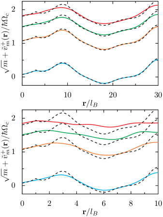
Figure 1: (Color online) Dimensionless effective potential $\xi_{m,+}({\bf r})/\hbar\Omega_{c}=\sqrt{m}+\tilde{v}_{m}^{+}({\bf r})/\hbar\Omega_{c}$ from Eq. (125) as a function of linear tip position ${\bf r}/l_{B}$ for the first Landau levels $m=0,1,2,3$ (bottom to top in full lines), and compared to the bare potential energy $\sqrt{m}+V_{s}({\bf r})/\hbar\Omega_{c}$ given by the dashed lines. The top panel corresponds to smooth disorder while the bottom one has stronger variations in the potential on the scale $l_{B}$ (see the relative axes).

The upper panel of Fig. 1, which corresponds to a (uni-dimensional) disordered scalar potential landscape $V_{s}({\bf r})$ smooth on the scale $l_{B}$, shows that the effective potential $\xi_{m,+}({\bf r})$ follows precisely the bare disorder potential for the lowest Landau level $m=0$, yet presents some moderate deviations for the following levels, illustrating the small averaging present on the larger scale of the quantum cyclotron radius $L_{m}=\sqrt{2m+1}l_{B}$. In contrast, the lower panel of Fig. 1 presents the situation of a disordered scalar potential landscape $V_{s}({\bf r})$ which has spatial variations comparable to $l_{B}$ [we stress again that the effective potential given by Eq. (93) and thus also by Eq. (125) has a truly non-perturbative character in $l_{B}$]. In that case, we can notice two effects: (i) the effective potential $\xi_{m,+}({\bf r})$ shows important quantitative deviations from the bare one already in the lowest Landau level $m=0$; (ii) at increasing $m>0$, stronger and stronger averaging effects take place, so that the effective potential $\xi_{m,+}({\bf r})$ rapidly flattens out. As a consequence, the typical energy width of the effective potentials $\xi_{m,\pm}({\bf r})$ as a function of position ${\bf r}$ clearly decreases with growing $m$. This effect is clearly seen in the STS data of Ref. Miller2009, for graphene and can be also recognized in recent measurements on standard 2DEGs by Hashimoto et al.Hash2008

We now discuss in more detail the STS spectra taken at fixed tip position, presented in the experimental papers Li2009 ; Miller2009 that showed a broadening of the Landau levels with a $\sqrt{m}$ scaling at increasing $m$. At high temperatures, such that $T\gg L_{m}\left|{\bm{\nabla}}\xi_{m,\pm}({\bf r})\right|$, the broadening has a purely thermal origin, with a fixed width set by $T$ and an exponential line shape (given by the Fermi function derivative). It is worth noting that the apparent increase with $m$ of the heights of the LDoS peaks in graphene Li2009 ; Miller2009 is solely due to the collapse of Landau levels, $E_{m+1}-E_{m}\propto 1/\sqrt{m}$ at large $m$, yet the underlying Landau peaks show a width insensitive to $m$.

Contrary to the discussion given in Ref. Li2009, , we emphasize that results of disorder averaged density of states, such as our Eq. (124) or the formula obtained, e.g., in Ref. Peres2006, , do not apply to account for the width of the STS peaks at fixed position, for which an expression for the local density of states, such as Eq. (119) or  (121), should instead be considered. In fact, the energy spread of the Landau-level peaks observed experimentally at low temperature in the LDoS can be easily understood to originate from wave-function broadening. Indeed, in formula (121) for instance, the polynomial $|H_{m}(x)|^{2}$ being of order $2m$, the squared wave function $f(x)=|H_{m}(x)|^{2}e^{-x^{2}}$ turns out to be spread on a characteristic scale $x_{m}=\sqrt{2m+1}$. We note that in Fig. 2 of Ref. Kramer2010, , a square-root dependence of the Landau-level widths with the Landau-level index can also be observed at zero-temperature (the oscillatory substructure of each Landau level peak disappears when including a small thermal smearing, as performed here). Turning to the LDoS expression (121), one sees that the effective energy width of the $m$th Landau-level peak is roughly given by the local energy scale $\sqrt{2m+1}l_{B}|{\bm{\nabla}}V_{s}({\bf r})|=L_{m}|{\bm{\nabla}}V_{s}({\bf r})|$ [here we have used the fact that the effective potential $\xi_{m,\pm}({\bf r})$ roughly follows the bare potential $V_{s}({\bf r})$], which scales as $\sqrt{m}$ as observed in the experiment. Li2009 This effect can be checked by a simple numerical evaluation of Eq. (121), taking into account the convolution with a thermal smearing as resulting from Eq. (118) for the STS local density of states. The obtained result for the sequence of LDoS peaks is shown in Fig. 2 for different temperatures.

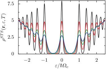
Figure 2: (Color online) Energy-dependent STS spectra for the local density of states $\rho^{STS}({\bf r},\varepsilon,T)$ at fixed tip position ${\bf r}$ from Eqs. (118) and (121) in units of $4/(2\pi l_{B}^{2})$ and as a function of energy $\varepsilon$ for several temperatures $T/\hbar\Omega_{c}=0.03,0.05,0.07,0.09$ (top to bottom). Here the local energy scale associated to the drift motion in the lowest Landau level is $\Gamma_{0}^{loc}({\bf r})=l_{B}|{\bm{\nabla}}V_{s}|=0.02\hbar\Omega_{c}$. At the lowest given temperature, the smearing with increasing $m$ of the Landau-level peaks is characterized by a local energy width which roughly grows as $\sqrt{m}$ (thermal smearing provides still some dominant contribution).

At temperatures comparable to $\Gamma^{\mathrm{loc}}_{0}({\bf r})\sim l_{B}|{\bm{\nabla}}V_{s}|$, quantum smearing due to the drift motion, which is encoded by the spatial dependence of the kernel $K_{m}({\bf R})$ in the general expression (119), or by the Hermite wave functions in the special case of a globally flat potential [see Eq. (121)], starts to appear. The growth of the energy width of the LDoS peaks at increasing Landau-level index $m$ is visible for the lowest chosen temperature in Fig. 2. In that case, one also sees a clear decrease in the heights of the LDoS peak with $m$, as observed experimentally. Li2009 ; Miller2009 ; Hash2008 Because the total smearing of the Landau levels depends both on thermal and intrinsic wave function broadening, the linewidth is only roughly behaving as $\sqrt{m}$.

Finally, we address the question of the Landau-levels line shape in the LDoS. In experiment of Ref. Li2009, , it has been pointed out that Lorentzian fits are significantly better than Gaussian ones to account quantitatively for the broadening of the LDoS peaks. On the other hand, in experiment by Miller et al. Miller2009 the line shape has been modeled by a convolution of Lorentzians and Gaussians to include extrinsic origins of broadening induced by temperature and instrumental resolution. On theoretical grounds, thermal broadening implies exponential line shapes (in between Lorentzians and Gaussians), while intrinsic wave function broadening of drift states (for non-vanishing local potential gradients) leads to Gaussian-type energy decay. We also note that spectra taken in regions of small potential gradients involve intrinsic exponential linewidth due to curvature effects, see Ref. Champel2009bis, for a discussion of the lowest Landau-level LDoS peak in the 2DEG. Therefore, it is difficult in general to disentangle the different contributions from the experiment, and systematic studies in temperature and as function of tip position, would be required to settle precisely this issue.

VII Conclusion

In this paper, we have extended to the graphene case a Green’s-function formalism well suited to study the mechanism of lifting of the Landau-level degeneracy by a smooth potential landscape at high magnetic fields, which was originally developed for the two-dimensional electron gases. The whole formalism relies on the use of a particular representation of semicoherent states, which are eigenstates of the kinetic part of the Hamiltonian. These so-called vortex states in the 2DEG case, or graphene vortex states in the graphene case, are both characterized by an integer topological quantum number $m$, related to the vortex circulation and giving rise to the Landau quantization of the orbital motion, and by a doubly continuous quantum number ${\bf R}$, corresponding to the location of the vortexlike phase singularities of the electronic wave function and characterizing the huge degeneracy of the Landau levels in the absence of disorder. The coherent states character with respect to the degeneracy quantum number ${\bf R}$ allows one to project the electron dynamics onto this overcomplete representation of states, which rigorously extends to quantum mechanics the classical guiding-center picture.

In a first stage, we have derived the exact matrix elements for smooth arbitrary scalar and mass potentials, as well as for off-diagonal smooth potentials related to ripples in graphene. The particular form of these matrix elements has revealed the different processes leading to Landau-level mixing and coupling between electron and hole bands. We have shown that at high magnetic field, when the Landau-level mixing can be safely neglected, a mixing between the hole and electron energy bands is unavoidably induced by second-order derivatives of the scalar potential, independently of the presence or not of a mass potential. We have been able to derive in this high magnetic field regime exact expressions for the electronic Green’s function in the presence either of an arbitrary quadratic scalar potential or an arbitrary quadratic mass potential.

Besides affording the derivation of unique Green’s function solutions valid for closed and open quadratic potentials which underline the dual correspondence between quantization effects and tunneling effects, we have emphasized that the semicoherent vortex representation offers a quasilocal perspective of the quantization process closely related to the deformation view of the classical phase-space mechanics, a property which turns out to be essential to capture the transition from the nonlocal quantum world to the local classical world. Furthermore, the vortex representation has revealed a hierarchy of local energy scales formed by the successive derivatives of the potential and thus ordered by their degree of nonlocality. As a result, quantum features associated with the lowest derivatives of the potential appear to be the most robust against the inelastic effects. We have emphasized that the consideration of a finite temperature allows one to disregard the smallest inaccessible energy scales and thus to devise successive approximation schemes for an arbitrary smooth potential.

Within this spirit, we have derived controlled analytical expressions for the local density of states in graphene valid at high magnetic field in the presence of smooth arbitrary scalar and mass potentials within different temperature regimes. We have identified the most relevant mechanism of intrinsic broadening of the LDoS peaks and have shown that a lot of information on the different potentials at play in graphene can be extracted from the experimental LDoS spectra performed at high magnetic field. Finally, we have been able to explain a few of the experimental findings, e.g., concerning the scaling of the LDoS peaks with the Landau-level index, recently observed Li2009 ; Miller2009 in scanning tunneling spectroscopy of graphene.

Appendix A Energy spectrum for closed quadratic potentials

In this appendix, we show how the energy spectrum for a confining quadratic potential (with a positive Gaussian curvature) can be determined from a retarded Green’s function expression such as given, e.g., by Eq. (95). For $\gamma_{0}({\bf R})>0$, the function

$$W({\bf R},t)=\frac{e^{-i\left[\eta_{0}({\bf R})/\gamma_{0}({\bf R})\right]\tau_{0}(t)}}{\cos\left(\sqrt{\gamma_{0}({\bf R})}t\right)}$$ (126)

is periodic in time with the period $T=2\pi/\sqrt{\gamma_{0}({\bf R})}$ at fixed ${\bf R}$. We thus expand it in a Fourier series

$$W({\bf R},t)=\sum_{p=-\infty}^{+\infty}a_{p}({\bf R})e^{-ip\sqrt{\gamma_{0}({\bf R})}t},$$ (127)

and insert expression (127) into Eq. (95) to straightforwardly get after integration over time

$$\tilde{g}_{0}({\bf R})=\sum_{p=-\infty}^{+\infty}\frac{a_{p}({\bf R})}{\omega-w_{0}({\bf R})-p\sqrt{\gamma_{0}({\bf R})}+i0^{+}}$$ (128)

with $w_{0}({\bf R})=\tilde{v}_{0}({\bf R})-\eta_{0}({\bf R})/\gamma_{0}({\bf R})$.

The Fourier coefficients $a_{p}({\bf R})$ are given by

$$a_{p}({\bf R}) = \frac{\sqrt{\gamma_{0}({\bf R})}}{2\pi}\int_{0}^{2\pi/\sqrt{\gamma_{0}({\bf R})}}\!\!\!\!dt\,W({\bf R},t)\,e^{ip\sqrt{\gamma_{0}({\bf R})}t}\hskip 19.91684pt$$ (129)

$$= \frac{\left[1-(-1)^{p}\right]}{2\pi}\int_{-\pi/2}^{\pi/2}\!\!\!\!d\theta\,\frac{e^{-i\rho({\bf R})\tan\theta}}{\cos\theta}\,e^{ip\theta}$$ (130)

with $\rho({\bf R})=\eta_{0}({\bf R})/\left[\gamma_{0}({\bf R})\right]^{3/2}$. We rewrite the following function appearing in the integrand of integral (130) as

$$\frac{e^{-i\rho({\bf R})\tan\theta}}{\cos\theta} = 2e^{\rho({\bf R})}\frac{e^{i\theta}}{1+e^{2i\theta}}\exp\left[-2\rho({\bf R})\frac{e^{2i\theta}}{1+e^{2i\theta}}\right]$$

$$= 2e^{-\rho({\bf R})}\frac{e^{-i\theta}}{1+e^{-2i\theta}}\exp\left[2\rho({\bf R})\frac{e^{-2i\theta}}{1+e^{-2i\theta}}\right].$$

It is then convenient to introduce the identity (see, e.g., Ref. Gradstein, )

$$\frac{1}{z-1}\exp\left(\frac{xz}{z-1}\right)=\sum_{n=0}^{+\infty}L_{n}(x)z^{n},$$ (133)

where $L_{n}(x)$ is the Laguerre polynomial of degree $n$. Formula (133) is usually defined for $|z|<1$, but it can be checked that it still holds for $z=e^{i\varphi}$ with $\varphi\neq 2\pi j$ ($j$ a positive or negative integer) at $x>0$. Indeed, using the asymptotic behavior of the Laguerre polynomials at large $n$ and $x>0$,

$$L_{n}(x)\approx\frac{e^{x/2}}{\sqrt{\pi}(nx)^{1/4}}\cos\left(2\sqrt{x\left(n+\frac{1}{2}\right)}-\frac{\pi}{4}\right),$$ (134)

we note that the series on the right-hand side of Eq. (133) is semi-convergent (this can be established using Abel’s test). On the other hand, for $x<0$, we have

$$L_{n}(x)\approx\frac{e^{-x/2}}{2\sqrt{\pi}(n|x|)^{1/4}}\exp\left(2\sqrt{|x|\left(n+\frac{1}{2}\right)}\right),$$ (135)

meaning that the series on the right-hand side of Eq. (133) is divergent for $x<0$ and $z=e^{i\varphi}$.

Using Eqs. (A) or (LABEL:exp2), and Eq. (133) by writing $x=2|\rho({\bf R})|$ and $z=-e^{-2i\chi\theta}$ depending on the sign of the quantity $\rho({\bf R})$ [we introduce the short-hand notation $\chi=\mathrm{sgn}\,\rho({\bf R})$], we can easily perform the integration over the angle $\theta$ in Eq. (130) and find

$$a_{p}({\bf R})=2(-1)^{n}e^{-\left|\rho({\bf R})\right|}L_{n}\left(2\left|\rho({\bf R})\right|\right)$$ (136)

for $p=\chi(2n+1)$ and $a_{p}({\bf R})=0$ for any values of $p\neq\chi(2n+1)$. Therefore, only the terms with $p=\chi(2n+1)$ remain in expression (128), where $n$ is a positive integer and $\chi=\pm 1$ is an index determining if the region is locally convex or concave.

Now, for the particular case of purely quadratic scalar and mass potentials, the poles of the Green’s function (128) are ${\bf R}$ independent, and thus directly yield the energy spectrum, Eq. (100), with the set of quantum numbers $(m,n)$ if the quadratic potential $V_{s}-V_{z}$ is convex, i.e., confining ($\chi=+1$ in this case).

Appendix B Solution for a locally quadratic scalar potential $V_{s}$

In this appendix, we solve the equations of motion, Eq. (86), in the regime where we can consider that the effective potential $\tilde{v}_{m}^{-}({\bf R})$ has a negligible spatial dispersion and that the effective potential $\tilde{v}_{m}^{+}({\bf R})$ can be locally described up to its second-order derivatives (i.e., it is locally written as a two-dimensional quadratic potential). These assumptions turn out to be exactly fulfilled in the particular case of a globally quadratic scalar potential $V_{s}({\bf R})$ and a constant mass term $V_{z}$, for which the matrix elements at high magnetic field read for $m\geq 1$,

$$\tilde{v}_{m}^{+}({\bf R}) = V_{s}({\bf R})+m\frac{l_{B}^{2}}{2}\Delta_{{\bf R}}V_{s}({\bf R}),$$ (137)

$$\tilde{v}_{m}^{-}({\bf R}) = -V_{z}+\frac{l_{B}^{2}}{4}\Delta_{{\bf R}}V_{s}({\bf R})=cst.$$ (138)

Using the explicit form, Eq. (64), of the $\star$ operator and the fact that $\tilde{v}^{+}_{m}({\bf R})$ is a quadratic function (so that all its derivatives higher than 3 vanish) and that $\tilde{v}^{-}_{m}({\bf R})$ is quasi-independent of ${\bf R}$, Eq. (86) becomes

$$\left(\omega-\tilde{v}_{m}^{+}({\bf R})-E_{m,\lambda_{1}}+i0^{+}\right)\,\tilde{g}_{m;\lambda_{1};\lambda_{2}}({\bf R})=\delta_{\lambda_{1},\lambda_{2}}+\tilde{v}_{m}^{-}\tilde{g}_{m;-\lambda_{1};\lambda_{2}}({\bf R})+i\frac{l_{B}^{2}}{2}\left[\partial_{X}\tilde{v}_{m}^{+}\partial_{Y}-\partial_{Y}\tilde{v}_{m}^{\mathrm{+}}\partial_{X}\right]\tilde{g}_{m;\lambda_{1};\lambda_{2}}({\bf R})$$

$$-\frac{l_{B}^{4}}{8}\left[\left(\partial_{Y}^{2}\tilde{v}_{m}^{+}\right)\partial_{X}^{2}+\left(\partial_{X}^{2}\tilde{v}_{m}^{+}\right)\partial_{Y}^{2}-2\left(\partial_{X}\partial_{Y}\tilde{v}_{m}^{+}\right)\partial_{X}\partial_{Y}\right]\tilde{g}_{m;\lambda_{1};\lambda_{2}}({\bf R}).$$ (139)

To solve Eq. (139), we introduce an arbitrary reference point ${\bf R}_{0}$ and write $\tilde{g}_{m;\lambda_{1};\lambda_{2}}({\bf R})=f_{m;\lambda_{1};\lambda_{2}}\left[E({\bf R})\right]$ with $E({\bf R})=\tilde{v}_{m}^{+}({\bf R})-\tilde{v}_{m}^{+}({\bf R}_{0})$. Substituting this form into Eq. (139), we get the system of differential equations,

$$\left[(\gamma_{m}^{+}E+\eta_{m}^{+})\frac{d^{2}}{dE^{2}}+\gamma_{m}^{+}\frac{d}{dE}-E+\omega-\tilde{v}_{m}^{+}({\bf R}_{0})-E_{m,\lambda_{1}}+i0^{+}\right]f_{m;\lambda_{1};\lambda_{2}}(E)-\tilde{v}_{m}^{-}f_{m;-\lambda_{1};\lambda_{2}}(E)=\delta_{\lambda_{1},\lambda_{2}},$$

(140)

where the geometric coefficients $\gamma_{m}^{+}$ and $\eta_{m}^{+}$ have the same definitions as in Eqs. (97) and (98) [with $\tilde{v}_{0}({\bf R})$ replaced by the effective potential $\tilde{v}_{m}^{+}({\bf R})$], and are expressed at the reference point ${\bf R}_{0}$. In the derivation of Eq. (140), we have used the relation $\eta_{m}^{+}({\bf R})=\eta_{m}^{+}+\gamma_{m}^{+}\left[\tilde{v}_{m}^{+}({\bf R})-\tilde{v}_{m}^{+}({\bf R}_{0})\right]$ which holds for any quadratic potential $\tilde{v}_{m}^{+}({\bf R})$. We then go to Fourier space by writing

$$f_{m;\lambda_{1};\lambda_{2}}(E)=\int d\tau F_{m;\lambda_{1};\lambda_{2}}(\tau)\,e^{-iE\tau},$$ (141)

and obtain a system of coupled first-order differential equations for $F$

$$\left[i(1+\gamma_{m}^{+}\tau^{2})\frac{d}{d\tau}+i\gamma_{m}^{+}\tau-\eta_{m}^{+}\tau^{2}+\omega-\tilde{v}_{m}^{+}({\bf R}_{0})-E_{m,\lambda_{1}}+i0^{+}\right]F_{m;\lambda_{1};\lambda_{2}}(\tau)$$

$$-\tilde{v}_{m}^{-}F_{m;-\lambda_{1};\lambda_{2}}(\tau)=\delta(\tau)\,\delta_{\lambda_{1},\lambda_{2}}.$$ (142)

Introducing into Eqs. (142) the (last) change in function,

$$F_{m;\lambda_{1};\lambda_{2}}(\tau)=\frac{h_{\lambda_{1};\lambda_{2}}\left[t(\tau)\right]}{\sqrt{1+\gamma_{m}^{+}\tau^{2}}}e^{i\left[\omega-\tilde{v}_{m}^{+}({\bf R}_{0})\right]t(\tau)}$$

$$\times e^{i\left(\eta_{m}^{+}/\gamma_{m}^{+}\right)\left[t(\tau)-\tau\right]}\hskip 14.22636pt$$ (143)

with

$$t(\tau)=\frac{1}{\sqrt{\gamma_{m}^{+}}}\arctan\left(\sqrt{\gamma_{m}^{+}}\tau\right),$$ (144)

we arrive at a simple linear system of two coupled first-order inhomogeneous differential equations with constant coefficients,

$$\left[i\frac{d}{dt}-\lambda E_{m}+i0^{+}\right]h_{\lambda;\lambda}(t)-\tilde{v}_{m}^{-}h_{-\lambda;\lambda}(t) = \delta\left[\tau(t)\right],\hskip 28.45274pt$$ (145)

$$\left[i\frac{d}{dt}+\lambda E_{m}+i0^{+}\right]h_{-\lambda;\lambda}(t)-\tilde{v}_{m}^{-}h_{\lambda;\lambda}(t) = 0$$ (146)

with

$$\tau(t)=\frac{1}{\sqrt{\gamma_{m}^{+}}}\tan\left(\sqrt{\gamma_{m}^{+}}t\right).$$ (147)

Note that $\delta\left[\tau(t)\right]=\delta(t)$ if $\gamma_{m}^{+}\leq 0$ and $\delta\left[\tau(t)\right]=\sum_{n}\delta\left(t-n\pi/\sqrt{\gamma_{m}^{+}}\right)$ if $\gamma_{m}^{+}>0$. Let us consider for the time being the case $\gamma_{m}^{+}\leq 0$. The solution of the system of Eqs. (145) and (146) leading to a well-defined integral (141) can then be readily derived and reads

$$\left(\begin{array}[]{c}h_{\lambda;\lambda}(t)\\ h_{\lambda;-\lambda}(t)\end{array}\right)=-\frac{i\theta(t)}{2}\left\{\left(\begin{array}[]{c}1+\lambda\alpha_{m}\\ \beta_{m}\end{array}\right)e^{-it\sqrt{E_{m}^{2}+\left[\tilde{v}_{m}^{-}\right]^{2}}}\right.$$ (152)

$$\left.+\left(\begin{array}[]{c}1-\lambda\alpha_{m}\\ -\beta_{m}\end{array}\right)e^{it\sqrt{E_{m}^{2}+\left[\tilde{v}_{m}^{-}\right]^{2}}}\right\}e^{-0^{+}t}.\hskip 14.22636pt$$ (155)

The expressions for the coefficients $\alpha_{m}$ and $\beta_{m}$ are given in Eqs. (102) and (103). Coming back to the original functions $\tilde{g}_{m;\lambda_{1};\lambda_{2}}({\bf R})$ and setting ${\bf R}={\bf R}_{0}$, we get the compact expression for the modified retarded Green’s function written in Eq. (101). For the case $\gamma_{m}^{+}>0$, it is important to realize that the relevant variable is the time $t$, not the variable $\tau$ (whereas it is possible to work indifferently with $t$ or $\tau$ for $\gamma_{m}^{+}\leq 0$). It can be checked that integral (101) is well defined as well for $\gamma_{m}^{+}\leq 0$ as for $\gamma_{m}^{+}>0$ [in the latter case the infinitesimal quantity $i0^{+}$ is crucial while it does not help to make the integral convergent when expressing the solution under the form of an integral over $\tau$ as within Eq. (141)].

Appendix C Solution for a locally quadratic mass term $V_{z}$

In this appendix, we solve the equations of motion, Eq. (86), in the regime where we can consider that the effective potential $\tilde{v}_{m}^{+}({\bf R})$ has a negligible spatial dispersion and that the effective potential $\tilde{v}_{m}^{-}({\bf R})$ can be locally described up to its second-order derivatives. This regime contains as a particular case the situation where the scalar potential $V_{s}({\bf R})$ is globally constant in space and the mass potential $V_{z}({\bf R})$ has a quadratic dependence on ${\bf R}$. In this particular case, we obviously get exactly that $\tilde{v}_{m}^{+}({\bf R})=cst$ and $\tilde{v}_{m}^{-}({\bf R})$ depends quadratically on the variable ${\bf R}$,

$$\tilde{v}_{m}^{+}({\bf R}) = V_{s}({\bf R})-\frac{l_{B}^{2}}{4}\Delta_{{\bf R}}V_{z}({\bf R})=cst,\hskip 17.07182pt$$ (156)

$$\tilde{v}_{m}^{-}({\bf R}) = -V_{z}({\bf R})-m\frac{l_{B}^{2}}{2}\Delta_{{\bf R}}V_{z}({\bf R}).\hskip 17.07182pt$$ (157)

In the regime considered in this appendix, Eq. (86) becomes

$$\left(\omega-\tilde{v}_{m}^{+}-E_{m,\lambda_{1}}+i0^{+}\right)\,\tilde{g}_{m;\lambda_{1};\lambda_{2}}({\bf R})=\delta_{\lambda_{1},\lambda_{2}}+\tilde{v}_{m}^{-}({\bf R})\tilde{g}_{m;-\lambda_{1};\lambda_{2}}({\bf R})+i\frac{l_{B}^{2}}{2}\left[\partial_{X}\tilde{v}_{m}^{-}\partial_{Y}-\partial_{Y}\tilde{v}_{m}^{-}\partial_{X}\right]\tilde{g}_{m;-\lambda_{1};\lambda_{2}}({\bf R})$$

$$-\frac{l_{B}^{4}}{8}\left[\left(\partial_{Y}^{2}\tilde{v}_{m}^{-}\right)\partial_{X}^{2}+\left(\partial_{X}^{2}\tilde{v}_{m}^{-}\right)\partial_{Y}^{2}-2\left(\partial_{X}\partial_{Y}\tilde{v}_{m}^{-}\right)\partial_{X}\partial_{Y}\right]\tilde{g}_{m;-\lambda_{1};\lambda_{2}}({\bf R}).$$ (158)

As in Appendix B, we introduce a reference point ${\bf R}_{0}$. It can then be guessed that the functions $\tilde{g}_{m;\lambda_{1};\lambda_{2}}({\bf R})$ are functionals of the potential $E({\bf R})=\tilde{v}_{m}^{-}({\bf R}_{0})-\tilde{v}_{m}^{-}({\bf R})$, i.e., we can write $\tilde{g}_{m;\lambda_{1};\lambda_{2}}({\bf R})=f_{m;\lambda_{1};\lambda_{2}}\left[E({\bf R})\right]$. The contributions in Eq. (158) involving the first-order derivatives of the function $\tilde{v}_{m}^{-}({\bf R})$ then vanish. Furthermore, we shall suppose that the equality (90) still holds in the present studied case, what can be justified a posteriori. The problem thus reduces to the resolution of a system of two coupled differential equations. Indeed, Eq. (158) yields the system of equations

$$\left[(\gamma_{m}^{-}E+\eta_{m}^{-})\frac{d^{2}}{dE^{2}}+\gamma_{m}^{-}\frac{d}{dE}-E+\tilde{v}_{m}^{-}({\bf R}_{0})\right]f_{m;-\lambda_{1};\lambda_{2}}(E)$$

$$-(\omega-\tilde{v}_{m}^{+}-E_{m,\lambda_{1}}+i0^{+})f_{m;\lambda_{1};\lambda_{2}}(E)=-\delta_{\lambda_{1},\lambda_{2}}\hskip 14.22636pt$$ (159)

with the coefficients $\gamma_{m}^{-}$ and $\eta_{m}^{-}$ expressed at the position ${\bf R}_{0}$ and given by the formulas (97) and (98) written for the potential $-\tilde{v}_{m}^{-}({\bf R})$ in place of $\tilde{v}_{0}({\bf R})$. Applying the Fourier transformation, Eq. (141), we arrive at the system,

$$\left[i(1+\gamma_{m}^{-}\tau^{2})\frac{d}{d\tau}+i\gamma_{m}^{-}\tau-\eta_{m}^{-}\tau^{2}+\tilde{v}_{m}^{-}({\bf R}_{0})\right]F_{m;-\lambda_{1};\lambda_{2}}(\tau)$$

$$-(\omega-\tilde{v}_{m}^{+}-E_{m,\lambda_{1}}+i0^{+})F_{m;\lambda_{1};\lambda_{2}}(\tau)=-\delta(\tau)\,\delta_{\lambda_{1},\lambda_{2}}.$$

Introducing into Eq. (C) the change in function

$$F_{m;\lambda_{1};\lambda_{2}}(\tau)=\frac{h_{\lambda_{1};\lambda_{2}}\left[s(\tau)\right]}{\sqrt{1+\gamma_{m}^{-}\tau^{2}}}e^{i\left[\tilde{v}^{-}_{m}({\bf R}_{0})+\eta_{m}^{-}/\gamma_{m}^{-}\right]s(\tau)}$$

$$\times e^{-i\left(\eta_{m}^{-}/\gamma_{m}^{-}\right)\tau}$$ (161)

with

$$s(\tau)=\frac{1}{\sqrt{\gamma_{m}^{-}}}\arctan\left(\sqrt{\gamma_{m}^{-}}\tau\right),$$ (162)

a simpler system of two coupled differential equations with constant coefficients comes out,

$$i\frac{d}{ds}h_{-\lambda;\lambda}(s)-(\omega-\tilde{v}_{m}^{+}-\lambda E_{m}+i0^{+})h_{\lambda;\lambda}(s)\hskip 42.67912pt$$

$$=-\delta\left[\tau(s)\right],\hskip 14.22636pt$$ (163)

$$i\frac{d}{ds}h_{\lambda;\lambda}(s)-(\omega-\tilde{v}_{m}^{+}+\lambda E_{m}+i0^{+})h_{-\lambda;\lambda}(s)=0.\hskip 14.22636pt$$ (164)

Note that, in contrast to the situation encountered in Appendix B, the variable $s$ does not have the meaning of the time here since it is no more conjugated to the frequency $\omega$ [this is the reason why we took care of naming the variable differently here although the expressions (147) and (162) are almost identical]. After diagonalization of the $2\times 2$ system, we obtain that the homogeneous solution of Eqs. (163) and (164) is

$$\left(\begin{array}[]{c}h_{\lambda;\lambda}(s)\\ h_{-\lambda;\lambda}(s)\end{array}\right)=C\left(\begin{array}[]{c}\omega-\tilde{v}_{m}^{+}+\lambda E_{m}\\ -\kappa_{m}\end{array}\right)e^{i\kappa_{m}s}$$ (169)

$$+D\left(\begin{array}[]{c}\omega-\tilde{v}_{m}^{+}+\lambda E_{m}\\ \kappa_{m}\end{array}\right)e^{-i\kappa_{m}s}$$ (172)

with $C$ and $D$ two arbitrary constants, and the energy $\kappa_{m}$ given by Eqs. (108) and (109) (we forget for the time being the infinitesimal quantity $i0^{+}$). The inhomogeneous solution of system of Eqs. (163) and (164) is then obtained by varying the constants $C(s)$ and $D(s)$. As a result, we get $C^{\prime}(s)=-D^{\prime}(s)=-i\delta(s)/(2\kappa_{m})$, that is $C(s)=\mp i\theta(\pm s)/(2\kappa_{m})$. Using that

$$\tilde{g}_{m;\lambda_{1};\lambda_{2}}({\bf R})=\int\!ds\frac{d\tau}{ds}F_{m;\lambda_{1};\lambda_{2}}(\tau(s))\,e^{i[\tilde{v}_{m}^{-}({\bf R})-\tilde{v}_{m}^{-}({\bf R}_{0})]\tau(s)},$$

the sign $\pm$ for the functions $C(s)$ and $D(s)$ is then chosen in such a way that integral (C) is convergent with the help of the infinitesimal quantity $i0^{+}$. Finally, taking the reference point ${\bf R}_{0}={\bf R}$ [so that $E({\bf R})=0$], we arrive at the expression (107) for the Green’s function, which holds irrespective of the sign of the coefficient $\gamma_{m}^{-}({\bf R})$.

Appendix D Simplifying the LDoS expression for locally flat potentials

In this appendix, we simplify further the expression (119) for the LDoS (valid for locally flat potentials) in the low-temperature regime within two different cases: (i) case of a potential landscape which varies slowly on the scale $L_{m}$ (Appendix D.1); (ii) case of a potential landscape which fluctuates spatially in a random way on the scale $L_{m}$ (Appendix D.2).

D.1 Potentials flat on the scale $L_{m}$

Writing the derivative of the Fermi-Dirac function as

$$n_{F}^{\prime}(\varepsilon-\xi_{m,\epsilon}({\bf R}))=-\frac{1}{2}\int_{-\infty}^{+\infty}\!\!\!\!\!\!dt\frac{Tt}{\sinh(\pi Tt)}\,e^{it\left[\varepsilon-\xi_{m,\epsilon}\left({\bf R}\right)\right]},$$

and using the linearization of the effective energy $\xi_{m,\epsilon}({\bf R}+{\bf r})\simeq\xi_{m,\epsilon}({\bf r})+{\bf R}.{\bm{\nabla}}\xi_{m,\epsilon}({\bf r})$ in Eq. (119), we can then perform the Gaussian integral over the vortex position ${\bf R}$ to get the LDoS expression,

$$\rho^{STS}({\bf r},\varepsilon,T)\simeq\frac{1}{2\pi l_{B}^{2}}\frac{4}{\pi}\int_{-\infty}^{+\infty}\!\!\!\!\!\!dt\left[e^{it(\varepsilon-\xi_{0}({\bf r}))}\exp\left\{-\frac{t^{2}\Gamma_{0}^{loc}({\bf r})^{2}}{4A_{s}}\right\}+\frac{1}{2}\sum_{m=1}^{+\infty}\sum_{\epsilon=\pm}\left\{(1+\epsilon\beta_{m})\frac{1}{m!}\frac{\partial^{m}}{\partial s^{m}}\right.\right.$$

$$\left.\left.\left.+(1-\epsilon\beta_{m})\frac{1}{(m-1)!}\frac{\partial^{m-1}}{\partial s^{m-1}}\right\}\frac{1}{1-s}e^{it(\varepsilon-\xi_{m,\epsilon}({\bf r}))}\exp\left\{-\frac{t^{2}\Gamma_{m,\epsilon}^{loc}({\bf r})^{2}}{4A_{s}}\right\}\right|_{s=0}\right]$$ (175)

with $\Gamma_{m,\epsilon}^{loc}({\bf r})=l_{B}|{\bm{\nabla}}\xi_{m,\epsilon}({\bf r})|$ and assuming temperature is low enough [i.e., $T\ll\Gamma_{m,\epsilon}^{loc}({\bf r})$] so that the limit $T\to 0$ can be taken. We then perform the integral over time $t$, and obtain:

$$\rho^{STS}({\bf r},\varepsilon,T)\simeq\frac{1}{2\pi l_{B}^{2}}\frac{4}{\sqrt{\pi}}\left[\frac{1}{\Gamma_{0}^{loc}({\bf r})}\exp\left\{-\left[\frac{\varepsilon-\xi_{0}({\bf r})}{\Gamma^{loc}({\bf r})}\right]^{2}\right\}+\frac{1}{2}\sum_{m=1}^{+\infty}\sum_{\epsilon=\pm}\frac{1}{\Gamma_{m,\epsilon}^{loc}({\bf r})}\left\{(1+\epsilon\beta_{m})\frac{1}{m!}\frac{\partial^{m}}{\partial s^{m}}\right.\right.$$

$$\left.\left.\left.+(1-\epsilon\beta_{m})\frac{1}{(m-1)!}\frac{\partial^{m-1}}{\partial s^{m-1}}\right\}\frac{1}{\sqrt{1-s^{2}}}\exp\left\{-A_{s}\left(\frac{\varepsilon-\xi_{m,\epsilon}({\bf r})}{\Gamma_{m,\epsilon}^{loc}({\bf r})}\right)^{2}\right\}\right|_{s=0}\right].\hskip 14.22636pt$$ (176)

Finally, using the following relation Gradstein obeyed by the Hermite polynomials $H_{n}(x)$

$$\frac{1}{\sqrt{1-s^{2}}}\exp\left[\frac{2sx^{2}}{1+s}\right]=\sum_{n=0}^{+\infty}\frac{(s/2)^{n}}{n!}\left[H_{n}(x)\right]^{2},$$ (177)

formula (176) can be recast in expression (121).

D.2 Potentials random on the scale $L_{m}$

We consider here the limit where the potential has strong spatial variations along the cyclotron radius, which applies to the situation of large Landau levels. We assume for simplicity that the antisymmetric part $V_{z}$ of the disorder potential can be neglected compared to the scalar component $V_{s}$ so that the effective potential given by Eq. (93) reads

$$\xi_{m,\pm}({\bf r}) = \pm E_{m}+\frac{1}{2}\int d^{2}{\bm{\eta}}V_{s}({\bm{\eta}})[K_{m}({\bf R}-{\bm{\eta}})$$ (178)

$$\hskip 14.22636pt+K_{m-1}({{\bf R}-\bm{\eta}})],$$

where $K_{-1}\equiv K_{0}$ in order for the above expression to apply for $m=0$ as well.

The averaging procedure is carried through the isotropic distribution function $S(q)$ in Fourier space (here $q=|{\bf q}|$) that describes the spatial correlations of disorder

$$\overline{V_{s}({\bf R_{1}})V_{s}({\bf R_{2}})}=S({\bf R_{1}}-{\bf R_{2}})=\int\frac{d^{2}{\bf q}}{(2\pi)^{2}}S(q)\,e^{i{\bf q}\cdot({\bf R_{1}}-{\bf R_{2}})}$$ (179)

so that the spatially averaged LDoS becomes

$$\rho^{DoS}(\omega) \equiv \overline{\rho({\bf r},\omega)}=-\frac{4}{\pi}\mathrm{Im}\int_{-\infty}^{+\infty}\!\!\!dt\int\!\!\!\frac{d^{2}{\bf R}}{2\pi l_{B}^{2}}\sum_{m=0}^{+\infty}\frac{1}{2}\sum_{\epsilon=\pm}$$

$$\times\int\mathcal{D}V_{s}\,[K_{m}({\bf R}-{\bf r})+K_{m-1}({\bf R}-{\bf r})]e^{i[\omega-\xi_{m,\epsilon}({\bf R})]t}$$

$$\times\exp\left\{-\frac{1}{2}\int d^{2}{\bf R_{1}}\int d^{2}{\bf R_{2}}\,S^{-1}({\bf R_{1}}-{\bf R_{2}})V_{s}({\bf R_{1}})V_{s}({\bf R_{2}})\right\}$$

where the distribution $S^{-1}$ obeys $\delta({\bf R})=\int d^{2}{\bm{\eta}}\;S^{-1}({\bf R}-{\bm{\eta}})S({\bm{\eta}})$. Inserting the effective potential, Eq. (178), and performing the functional integral over the disorder realizations, we obtain

$$\rho^{DoS}(\omega) = -\frac{4}{\pi}\mathrm{Im}\int_{-\infty}^{+\infty}\!\!\!dt\int\!\!\!\frac{d^{2}{\bf R}}{2\pi l_{B}^{2}}\sum_{m=0}^{+\infty}\frac{1}{2}\sum_{\epsilon=\pm}e^{i[\omega-\epsilon E_{m}]t}$$

$$\times[K_{m}({\bf R}-{\bf r})+K_{m-1}({\bf R}-{\bf r})]\exp\left\{-\frac{1}{4}t^{2}\,[\Gamma_{m}^{DoS}]^{2}\right\}$$

where the width $\Gamma_{m}^{DoS}$ is given by Eq. (123). The above expression has obviously become ${\bf r}$ independent so that the ${\bf R}$ integral can be carried using the normalization condition $\int d^{2}{\bf R}K_{m}({\bf R})=1$. The remaining time integral gives the final result quoted in Eq. (VI.2.4).

References

- (1) K. S. Novoselov, A. K. Geim, S. V. Morozov, D. Jiang, M. I. Katsnelson, I. V. Grigorieva, S. V. Dubonos, and A. A. Firsov, Nature (London) 438, 197 (2005); K. S. Novoselov, E. Mc-Cann, S. V. Morozov, V. I. Falko, M. I. Katsnelson, U. Zeitler, D. Jiang, F. Schedin, and A. K. Geim, Nat. Phys. 2, 177 (2006).
- (2) Y. Zhang, Y.-W. Tan, H. L. Stormer, and P. Kim, Nature (London) 438, 201 (2005); Y. Zhang, Z. Jiang, J. P. Small, M. S. Purewal, Y.-W. Tan, M. Fazlollahi, J. D. Chudow, J. A. Jaszczak, H. L. Stormer, and P. Kim, Phys. Rev. Lett. 96, 136806 (2006).
- (3) K. S. Novoselov, Z. Jiang, Y. Zhang, S. V. Morozov, H. L. Stormer, U. Zeitler, J. C. Maan, G. S. Boebinger, P. Kim, and A. K. Geim, Science 315, 1379 (2007).
- (4) A. H. Castro Neto, F. Guinea, N. M. R. Peres, K. S. Novoselov, and A. K. Geim, Rev. Mod. Phys. 81, 109 (2009).
- (5) Y. Zheng and T. Ando, Phys. Rev. B 65, 245420 (2002).
- (6) V. P. Gusynin and S. G. Sharapov, Phys. Rev. Lett. 95, 146801 (2005).
- (7) K. Hashimoto, C. Sohrmann, J. Wiebe, T. Inaoka, F. Meier, Y. Hirayama, R. A. Römer, R. Wiesendanger, and M. Morgenstern, Phys. Rev. Lett. 101, 256802 (2008).
- (8) A. W. W. Ludwig, M. P. A. Fisher, R. Shankar, and G. Grinstein, Phys. Rev. B 50, 7526 (1994).
- (9) P. Goswami, X. Jia, and S. Chakravarty, Phys. Rev. B 76, 205408 (2007).
- (10) A. J. M. Giesbers, U. Zeitler, L. A. Ponomarenko, R. Yang, K. S. Novoselov, A. K. Geim, and J. C. Maan, Phys. Rev. B 80, 241411(R) (2009).
- (11) G. Li, A. Luican, and E. Y. Andrei, Phys. Rev. Lett. 102, 176804 (2009).
- (12) D. L. Miller, K. D. Kubista, G. M. Rutter, M. Ruan, W. A. de Heer, P. N. First, and J. A. Stroscio, Science 324, 924 (2009).
- (13) T. Ohta, A. Bostwick, T. Seyller, K. Horn, and E. Rotenberg, Science 313, 951 (2006).
- (14) S. V. Morozov, K. S. Novoselov, M. I. Katsnelson, F. Schedin, L. A. Ponomarenko, D. Jiang, and A. K. Geim, Phys. Rev. Lett. 97, 016801 (2006).
- (15) V. Lukose, R. Shankar, and G. Baskaran, Phys. Rev. Lett. 98, 116802 (2007).
- (16) N. M. R. Peres, and E. V. Castro, J. Phys.: Condens. Matter 19, 406231 (2007).
- (17) P. Recher, J. Nilsson, G. Burkard, and B. Trauzettel, Phys. Rev. B 79, 085407 (2009).
- (18) S. Schnez, K. Ensslin, M. Sigrist, and T. Ihn, Phys. Rev. B 78, 195427 (2008).
- (19) H.-Y. Chen, V. Apalkov, and T. Chakraborty, Phys. Rev. Lett. 98, 186803 (2007).
- (20) V. P. Gusynin and S. G. Sharapov, Phys. Rev. B 73, 245411 (2006).
- (21) R. R. Biswas and A. Balatsky, Phys. Rev. B 80, 081412(R) (2009).
- (22) C. Bena, Phys. Rev. B 81, 045409 (2010).
- (23) N. M. R. Peres, F. Guinea, and A. H. Castro Neto, Phys. Rev. B 73, 125411 (2006).
- (24) P. M. Ostrovsky, I. V. Gornyi, and A. D. Mirlin, Phys. Rev. B 77, 195430 (2008).
- (25) M. E. Raikh and T. V. Shahbazyan, Phys. Rev. B 47, 1522 (1993).
- (26) T. Champel and S. Florens, Phys. Rev. B 80, 125322 (2009).
- (27) T. Champel and S. Florens, Phys. Rev. B 75, 245326 (2007).
- (28) T. Champel, S. Florens, and L. Canet, Phys. Rev. B 78, 125302 (2008).
- (29) S. M. Girvin and T. Jach, Phys. Rev. B 29, 5617 (1984).
- (30) J. K. Jain and S. A. Kivelson, Phys. Rev. B 37, 4111 (1988).
- (31) T. Champel and S. Florens, Phys. Rev. B 80, 161311(R) (2009).
-
(32)
More precisely, the (non-normalized) Landau states read in the symmetrical gauge
where is a real number having the dimension of a momentum and is the Hermite polynomial of degree . Note that using the Landau gauge [] instead of the symmetrical gauge allows one to get rid of the exponential factor on the right-hand side of the above equation, as usually done in the literature. -
(33)
In the symmetrical gauge, the (non-normalized) circular states can be written as
where we have used the polar coordinates , is a positive or negative integer, is a positive integer, and is the generalized Laguerre polynomial of degree . Here, the eigenstates, in the above equation, of Hamiltonian (8) are associated with Landau levels energy quantization, Eq. (9), via the condition - (34) For a proof, see, e.g., Sec. II.D of Ref. Champel2007, .
- (35) T. M. Rusin, and W. Zawadzki, Phys. Rev. B 78, 125419 (2008).
- (36) J. Schliemann, New J. Phys. 10, 043024 (2008).
- (37) B. Dóra, K. Ziegler, P. Thalmeier, and M. Nakamura, Phys. Rev. Lett. 102, 036803 (2009).
- (38) We recently became aware of a very stimulating paper by Raikh and Shabazyan, Ref. Raikh1995, , where a formula analogous to Dyson equation, Eq. (63), was derived for the 2DEG with a different yet related method that starts with Landau states wave packets instead of vortex states. In their Eq. (2.8) can be recognized precisely our star-differential operator (64), written in Fourier space. These authors limited their analysis to the drift states (locally flat disordered potentials), neglecting curvature effects, a further step that was taken in our recent paper (Ref. Champel2009, ). They managed however, in a “tour de force” calculation, to compute the localization length in the tails of the Landau bands.
- (39) F. Bayen, M. Flato, C. Fronsdal, A. Lichnerowicz, and D. Sternheimer, Ann. Phys. (N.Y.) 111, 61 (1978) ; 111, 111 (1978).
- (40) C. Zachos, Int. J. Mod. Phys. A 17, 297 (2002).
- (41) C. Zachos, J. Math. Phys. 41, 5129 (2000).
- (42) J. E. Moyal, Proc. Cambridge Philos. Soc. 45, 99 (1949).
- (43) A. C. Hirshfeld and P. Henselder, Am. J. Phys. 70, 537 (2002).
- (44) A. Feldman and A. H. Kahn, Phys. Rev. B 1, 4584 (1970).
- (45) S. Varro, J. Phys. A 17, 1631 (1984).
- (46) T. Kramer, C. Kreisbeck, V. Krueckl, E. J. Heller, R. E. Parrott, and C.-T. Liang, Phys. Rev. B 81, 081410(R) (2010).
- (47) I. S. Gradshteyn and I. M. Ryzhik, Table of Integrals, Series, and Products (Academic Press, New York, 1980).
- (48) Handbook of Mathematical Functions, edited by M. Abramowitz and I. A. Stegun (Dover, New York, 1972).
- (49) M. E. Raikh and T. V. Shahbazyan, Phys. Rev. B 51, 9682 (1995).