Suppression of Kondo screening by the Dicke effect in multiple quantum dots

Abstract

The interplay between the coupling of an interacting quantum dot to a conduction band and its connection to localized levels has been studied in a triple quantum dot arrangement. The electronic Dicke effect, resulting from quasi-resonant states of two side-coupled non-interacting quantum dots, is found to produce important effects on the Kondo resonance of the interacting dot. We study in detail the Kondo regime of the system by applying a numerical renormalization group analysis to a finite-$U$ multi-impurity Anderson Hamiltonian model. We find an extreme narrowing of the Kondo resonance, as the single-particle levels of the side dots are tuned towards the Fermi level and “squeeze” the Kondo resonance, accompanied by a strong drop in the Kondo temperature, due to the presence of a supertunneling state. Further, we show that the Kondo temperature vanishes in the limit of the Dicke effect of the structure. By analyzing the magnetic moment and entropy of the three-dot cluster versus temperature, we identify a different local singlet that competes with the Kondo state, resulting in the eventual suppression of the Kondo temperature and strongly affecting the spin correlations of the structure. We further show that system asymmetries in couplings, level structure or due to Coulomb interactions, result in interesting changes in the spectral function near the Fermi level. These strongly affect the Kondo temperature and the linear conductance of the system.

I Introduction

Quantum dots (QDs) have played a prominent role in the investigation of the Kondo problem physics in recent years, DGG ; Inoshita ; Sasaki ; Cronenwett ; Pustilnik as they allow a systematic and well-controlled variation of structure parameters, with the consequent exploration of electronic correlations in this paramount many-body state. This exploration is of course possible by being able to experimentally tune the relevant parameters in the system over rather wide ranges. Moreover, in a feature that is unique to these systems, QDs also facilitate the incorporation and study of quantum coherence effects in the Kondo state, and its interplay with structure resonances and field-induced phase shifts. In fact, the Kondo effect has been studied in multi-quantum dot systems, including double,busser ; jeong ; cornaglia ; vernek ; 8l ; sasaki3 ; zitko5 and triple dots, kuzmenko1 ; jiang ; zitko2 ; lobos ; Vernek1 ; Numata ; Chiappe1 ; klaus ; haug in different geometrical arrangements, motivated in part by the richness of the Kondo physics in the presence of localized levels, as well as by their potential application as spin filters.

One of the main signatures of the Kondo state is the enhancement of the quasi-particle density of states at the Fermi level; this Kondo resonance is accessible in electronic transport experiments, as it opens an additional transport channel, which is readily seen in the differential conductance of these structures (typically in the zero-bias limit). In the case of multiple QD geometries, the Kondo and other single-particle–like resonances provide different transport channels which can even interfere with one another. As a result, these structures offer the interesting possibility of controlling the transport properties by exploiting quantum interference in the electronic propagation, allowing the study of scattering phenomena such as the well-known Fano fano and Aharonov-Bohm effects,Hofstetter ; 17' competing with the Kondo effect. For example, the interference of Kondo and Fano resonances in suitably designed structures has been shown recently in beautiful experiments, giving rise to complex conductance features.sato ; sasaki3 These results demonstrate that consideration of multiple coherent scattering of traveling electronic waves, both through single-particle as well as many-body resonances, is crucial for the understanding of the resulting conductance features. In this regard, being able to tune the structure parameters of a multiple QD system, as well as its Kondo state, provides a unique arena to study correlations and coherence effects in a controllable manner.

It is clear that the features of the Kondo resonance near the Fermi level significantly affect the conductance of the system, sometimes in quite subtle ways. For example, the shape of the density of states in the leads near the FL has been shown to produce strong modifications of the Kondo resonance and characteristic energy (the Kondo temperature). These modifications can arise from intrinsic global properties,WF ; Ingersent or from the local environment in the vicinity of the active QD.8l We are here especially interested in resonances and modifications due to the electronic version of the Dicke effect. orellana The latter is the electronic analogue of the well-known Dicke effect in quantum optics, which takes place in the spontaneous emission of closely-linked atoms lying in the same environment (within one characteristic wavelength of each other).dicke In the electronic case, the decay rates (level broadenings) are produced by the couplings between localized levels and a conduction channel, and their close proximity and effective coupling gives rise to effectively fast (super-tunneling) and slow (sub-tunneling) modes.18S ; 18C ; Brandes Interestingly, this coherent single-particle physics results in strong changes of the Kondo screening, as we will discuss below, once Coulomb interactions are fully taken into account.

Although other multidot geometries would exhibit similar physics, a specific configuration to study this effect consists of three QDs where two large (essentially non-interacting) dots are attached laterally to a central dot that is embedded between current leads, as schematically shown in Fig. 1. This cross-bar structure is reminiscent of quantum wave guides with a resonator cavity. Debray In our case, the side QDs act as scattering centers to the main transport channel, and compete with the Kondo effect of the central dot.torio Similar configurations have been studied before, and recent work by Trocha and Barnas using a slave boson mean field approach has identified interesting regimes.Trocha They studied the interplay between Kondo and Dicke resonances and considered the limit of infinite Coulomb repulsion ($U\rightarrow\infty$), which suppresses virtual processes involving the doubly occupied state in the interacting dot. Additionally, the mean-field approximation adopted in the auxiliary boson fields neglects correlations due to charge fluctuations involving the empty state of the dot. All of these processes may be expected to be important in providing a full description of the Kondo resonance, especially in competition with the Dicke effect here, as we indeed show in this work. Our numerical renormalization group (NRG) approach, Wilson ; Murthy ; 24B provides a reliable description that incorporates all charge and spin fluctuations in the problem, it allows the study of finite $U$ values–corresponding to real QD experiments–and gives us a systematic way to study the subtle interference effects inherent in this geometry.

In this work, we explore the Kondo state that appears when the levels of the non-interacting dots are brought together both symmetrically and asymmetrically about the Fermi level. In both situations, the Kondo resonance narrows drastically and is “squeezed” between the two single-particle levels, suggesting a drop in the Kondo temperature of the system, as described recently in the symmetric case.Trocha We show that indeed the Kondo temperature drops, as the onset of the Dicke effect involving the interacting dot totally suppresses the Kondo state and results in vanishing Kondo temperature. This behavior, due to the enhancement of spin-spin correlations in the QDs orbitals, results in the formation of a local singlet, which decouples from the current leads. As the system moves away from a fully degenerate Dicke configuration, the Kondo temperature is non-zero but has a non-monotonic dependence on structure parameters, behavior which is only brought out by our numerical renormalization group approach. This optimization of the Kondo effect in a structure may have interesting applications in a real experimental system.

We will further show that the competition of Kondo and Dicke effects modifies excited states near the Kondo regime as well, resulting in unexpected changes in the thermodynamic and transport properties of the system. Interestingly, the local (non-Kondo) singlet state mentioned above emerges due to a strong coupling between the interacting QD and the super-tunneling state. A crossover between these two configurations can be tuned by varying the coupling between the QDs.

We also describe the effects of asymmetries in the system, including different interdot couplings, as well as energy levels and finite Coulomb interactions in all the dots of the structure. We show that these structural asymmetries introduce interesting particle-hole asymmetries in the problem, resulting in strong changes in the Kondo temperatures and the linear conductance of the system.

II Model and theoretical approach

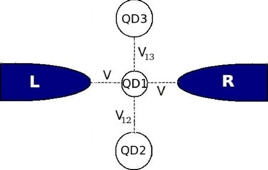
Figure 1: (color online) Schematic representation of the three-dot system. QD1 is considered to be strongly interacting ($U\neq 0$), whereas QD2 and QD3 are assumed to be effectively non-interacting ($U^{\prime}$ small or vanishing–see text).

The system consists of an interacting QD (labeled QD1) coupled to two current leads ($L$ and $R$) and to two effectively non-interacting QDs (QD2 and QD3) (see Fig. 1); one could also think of QD2 and QD3 as being close to a Coulomb blockade peak, so that they conduct and their behavior is single-resonance–like, as charging effects are typically small when conducting. The three-dot structure is described by a multi-impurity Anderson Hamiltonian, $H=H_{dots}+H_{leads}+H_{T}$, with

$$H_{dots} = \sum_{\sigma,i=1}^{3}\varepsilon_{i}c^{\dagger}_{i\sigma}c_{i\sigma}+U_{i}n_{i\uparrow}n_{i\downarrow}+$$ (1)

$$+\sum_{\sigma}\left[V_{12}c^{\dagger}_{1\sigma}c_{2\sigma}+V_{13}c^{\dagger}_{1\sigma}c_{3\sigma}+h.c.\right],$$

$$H_{leads} = \sum_{{k\sigma},\ell=R,L}\varepsilon_{\ell k}c^{\dagger}_{\ell k\sigma}c_{\ell k\sigma}$$ (2)

$$H_{T} = V\sum_{\ell k\sigma\atop\sigma}\left[c^{\dagger}_{1\sigma}c_{\ell k\sigma}+h.c.\right],$$ (3)

where $c^{\dagger}_{i\sigma}$ ($c_{1\sigma}$) is the operator that creates (annihilates) an electron with energy $\varepsilon_{i}$ ($i=1,2,3$) and spin $\sigma$ in the respective QD and $c^{\dagger}_{\ell k\sigma}$ is the corresponding fermion operator for the leads $\ell=R,L$, with energy $\varepsilon_{\ell k}$, where $k$ is the momentum quantum number of the free conduction electrons. The second term in Eq. (1) accounts for the Coulomb repulsion in the doubly occupied state of the dots. The hopping amplitudes $V$, $V_{12}$ and $V_{13}$ couple the interacting QD1 to the leads and to QD2 and QD3, respectively. For simplicity, unless stated otherwise (see Sec. III.2), we will take $V_{12}=V_{13}=V^{\prime}$, and $U_{1}=U\neq 0$, while $U_{2}=U_{3}=0$.

The characteristic properties of the Kondo physics of the system will be probed through thermodynamic quantities, namely the local magnetic moment and its contribution to the entropy, which can be readily obtained from the NRG procedure. To calculate dynamical quantities, such as the spectral functions and the conductance of the system, one needs to calculate the local retarded Green’s function (GF) at the interacting dot, which is defined in the standard form,

$$G_{11}^{\sigma}(\omega) \equiv \langle\langle c_{1\sigma};c^{\dagger}_{1\sigma}\rangle\rangle_{\omega}$$ (4)

$$= \int_{-\infty}^{\infty}e^{-i\omega\tau}\langle\langle c_{1\sigma}(t);c^{\dagger}_{1\sigma}(t^{\prime})\rangle\rangle d\tau,$$

where $\tau=t-t^{\prime}$, and

$$\langle\langle c_{1\sigma}(t);c^{\dagger}_{1\sigma}(t^{\prime})\rangle\rangle=-i\Theta(t-t^{\prime})\langle[c_{1\sigma}(t),c^{\dagger}_{1\sigma}(t^{\prime})]_{+}\rangle$$ (5)

is the double-time Green’s function, with $\Theta(\tau)$ the usual step function, and $[\cdots,\cdots]_{+}$ the anticommutator. Once $G_{11}^{\sigma}(\omega)$ is known, the spectral function $\rho_{1\sigma}(\omega)$ [or density of states (DOS)] of the interacting dot can be obtained from the relation

$$\rho_{1\sigma}(\omega)=-\frac{1}{\pi}{\tt Im}[G_{11}^{\sigma}(\omega)].$$ (6)

II.1 Non-interacting analysis

In the non-interacting limit ($U_{i}\rightarrow 0$) the GF $G_{11}^{(0)\sigma}(\omega)$ can be easily obtained by the equation-of-motion method, leading to an exact closed expression,

$$G^{(0)\sigma}_{11}(\omega)=\frac{1}{\omega-\varepsilon_{1}-\Sigma_{1}(\omega)},$$ (7)

where

$$\Sigma_{1}(\omega)=\Lambda_{1}(\omega)+i\Delta_{1}(\omega)$$ (8)

is the self-energy in the non-interacting case, which takes into account the effects of the QD1 contacts with the leads, and with QD2 and QD3. The self-energy can be written as

$$\Sigma_{1}(\omega)=2V^{2}\sum_{k}\frac{1}{\omega-\varepsilon_{k}}+V^{\prime 2}\frac{2\omega-\varepsilon_{2}-\varepsilon_{3}}{(\omega-\varepsilon_{2})(\omega-\varepsilon_{3})}.$$ (9)

In these expressions, the frequency $\omega$ must be understood in its analytical continuation sense, $\omega\rightarrow\omega+i\eta$, where $\eta$ is an infinitesimal. Notice that the poles at $\varepsilon_{2}$ and $\varepsilon_{3}$ appearing in the self-energy describe localized states in the effective conduction band due to the presence of QD2 and QD3. In the limit of $V^{\prime}\rightarrow 0$, the self-energy reduces to the single impurity case,

$$\Sigma_{1}^{(V^{\prime}=0)}(\omega)=\frac{\Delta_{0}}{2\pi}\ln\left|{\frac{\omega+D}{\omega-D}}\right|-i\Delta_{0},$$ (10)

where $\Delta_{0}=2\pi V^{2}/2D$ is the hybridization function for a flat density of states, and $D$ is the half-bandwidth of the conduction electrons. Notice that the effect of the leads and the two side-coupled QDs is fully taken into account in Eq. (7) by the self-energy $\Sigma_{1}(\omega)$, which provides a “structured” effective conduction band. The electrons localized in QD1 are then coupled via the effective density of states in the leads represented by $\Delta_{1}$ in Eq. (8).

The spectral function, $\rho_{1}^{0}\equiv\rho_{\uparrow}=\rho_{\downarrow}$ in this non-interacting case is depicted in Fig. 2 for $\epsilon_{1}=0$, $V^{\prime}=0.05$, $V=0.1$ and different values of $\delta$. We observe that by increasing $\delta$ the width of the central peak increases, while the satellite peaks are just slightly shifted away from the Fermi level. The shift of the satellite peak position can be estimated by analyzing the poles of $G_{11}^{\sigma}$. Assuming the satellite peaks to be Lorentzian-shaped, we find that their positions are given by $\pm\sqrt{2V^{\prime 2}+\delta^{2}}$. In the inset we show the peak positions as function of $\delta$. The continuous (black) curve corresponds to the analytical expression $1.01\sqrt{2V^{\prime 2}+\delta^{2}}$, while symbols correspond to the values obtained from the curves in the main panel. The need for the factor 1.01 results from the assumption that the peak has a Lorentzian shape in the analytical estimate. On the other hand, close to zero energy ($\omega\sim 0$) and for small detuning ($\delta\ll\Delta_{0}$), the DOS can be written as a superposition of a symmetric Fano lineshape–arising from the super-tunneling Dicke state–of width $\Gamma_{+}\propto\Delta_{0}$, and a Lorentzian line–arising from the subtunneling state– of width $\Gamma_{-}\propto\delta^{2}/\Delta_{0}$, respectively.orellana This complex behavior of the DOS is due to the hybridization of the lateral dots through the continuum of the central dot and leads. This phenomenon is in close analogy to the Dicke effect in quantum optics.orellana Here, the super-tunneling and subtunneling modes give rise a broad ($\Gamma_{+}$) antiresonance and a sharp ($\Gamma_{-}$) resonance, respectively. As we will discuss later, this effect also modifies dramatically the many-body Kondo state.

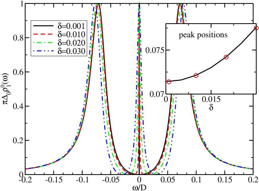
Figure 2: (color online) Spectral function vs. energy for $V=0.1$, $V^{\prime}=0.05$ and $\epsilon_{1}=0$, for $\delta=0.001$ (solid, black), $\delta=0.01$ (dashed, red), $\delta=0.02$ (dot-dash, green), and $\delta=0.03$ (dot-dot-dash, blue). The inset shows the position of the right-side satellite peak as function of $\delta$. Solid line corresponds to the analytical expression (see text) while (red) circles show peak positions taken from curves in main panel.

II.2 Interacting central dot

We will now consider the interesting case of interactions in the central dot only, so that $U_{1}=U$ is finite, while $U_{2}=U_{3}=U^{\prime}=0$. In this case, the system can also be mapped into a single QD coupled to an effective conduction band. In this case the dressed GF of the interacting dot can be formally written as:

$$G_{11}^{\sigma}(\omega)=\frac{1}{\omega-\varepsilon_{1}-\Sigma^{*}_{1}(\omega)},$$ (11)

where $\Sigma^{*}_{1}(\omega)$ is the proper self-energy which takes into account the influence of the lateral QDs, the current leads, as well as the Coulomb repulsion $U$. Unlike the non-interacting case, a closed expression for $\Sigma^{*}_{1}(\omega)$ is not possible, due to the many-body term in the Hamiltonian. However, $G_{11}^{\sigma}(\omega)$ can be reliably obtained using the NRG procedure.24B ; Jayaprakash For convenience, we write the GF in the Lehmann representation,Fetter

$$G_{11}^{\sigma}(\omega)=\frac{1}{Z}\sum_{nn^{\prime}}\frac{\mid\langle n|c^{\dagger}_{d\sigma}|n^{\prime}\rangle\mid^{2}}{\omega-E_{n^{\prime}}+E_{n}}\left(e^{-\beta E_{n}}+e^{-\beta E_{n^{\prime}}}\right),$$ (12)

where $Z$ is the partition function in the canonical ensemble, $|n\rangle$ is an eigenstate of the Hamiltonian $H$, with corresponding eigenenergy $E_{n}$, and $\beta=(k_{B}T)^{-1}$. The imaginary part of $G_{11}^{\sigma}(\omega)$ is calculated at zero temperature ($T=0$) directly from the NRG spectrum, Bulla1 while the real part can be obtained from a Kramers-Krönig transformation.Kramers

II.3 Cluster impurity approach

As we will see in the next section, it is also useful to analyze the details of the states involving the three QDs, considering the system as a whole. This approach also proves essential when dealing with Coulomb interactions in all three QDs, as the approach of an effective density of states described in the previous section, is no longer applicable in the more general case. To that end, we solve the problem considering all the dots composing the “impurity region,” so that the three-dot cluster is coupled to a flat conduction band. This requires a simple generalization of the NRG procedure: start with a cluster impurity described by a set of 64 basis states, on which one writes and diagonalizes the initial Hamiltonian, $H_{dots}$, while the current lead is characterized by a flat density of states. For these NRG “cluster impurity” runs, we typically keep 1600 states and use a discretization parameter $\Lambda=3.5$, which provides sufficient accuracy for the spectral function in the scales of interest.

III The role of electronic interactions

III.1 Particle-hole symmetric case

Hereafter, we set $D=1$ (typically the largest energy scale of the problem) as our energy unit. We further consider the Coulomb repulsion $U=0.5$, and $\varepsilon_{1}=-U/2$, which corresponds to a particle-hole symmetric system with interactions in QD1. In order to study the Dicke effect in this system we first focus on the particle-hole symmetric point of the entire system. To this end, we tune the on-site energies $\varepsilon_{2}$ and $\varepsilon_{3}$ of the non-interacting QDs ($U^{\prime}=0$) symmetrically displaced from the Fermi level, for which we set $\varepsilon_{3}=-\varepsilon_{2}=\delta$. With this choice of parameters, the last term of Eq. (9) shows two poles located at $\omega=\pm\delta$, which produce strong enhancement of the effective coupling $\Delta_{1}(\omega)$. This results in a dramatic distortion of the local interacting DOS projected in QD1, $\rho_{1}^{\sigma}(\omega)$, with important implications on the properties of the system.

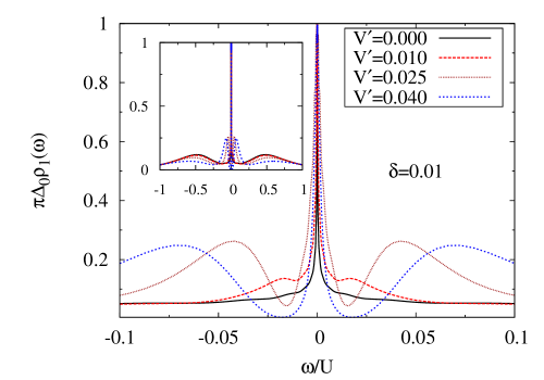
Figure 3: (color online) Spectral function vs. energy for $V=0.1$, $\delta=0.01$ and coupling $V^{\prime}=0.0$ (solid, black), $V^{\prime}=0.01$ (dashed, red), $V^{\prime}=0.025$ (dotted, brown) and $V^{\prime}=0.04$ (short-dash, blue). The inset shows the same curves over a wider energy range. Here, $U=0.5$, $U^{\prime}=0$, and $D=1$.

We first fix $\delta$ ($=0.01$) and vary the interdot coupling $V^{\prime}$. Figure 3 shows $\rho_{1}(\omega)$ ($=\rho_{1\uparrow}=\rho_{1\downarrow}$ in Eq. 6), for several values of $V^{\prime}$. The solid (black) curve shows the case $V^{\prime}=0$, which corresponds to the typical case of a QD coupled to a conduction band with a flat density of states. Notice the Kondo resonance at the Fermi level in addition to the two Hubbard peaks at $\approx\pm U/2$ (see inset; which give rise to Coulomb blockade peaks in the conductance at appropriate gate voltages). The width of the Kondo peak is proportional to the Kondo temperature, which in this case is T_K $T_{K}^{0}\equiv T_{K}(V^{\prime}=0)=5.6\times 10^{-5}$. As $V^{\prime}$ increases, the low-energy structure of $\rho_{1}(\omega)$ is strongly modified. Two satellite peaks emerge symmetrically about the central peak at $\omega=0$. These peaks become more pronounced for larger $V^{\prime}$ and the distance between them increases somewhat more than $2\sqrt{2{V^{\prime}}^{2}+\delta^{2}}$, as one would expect from the non-interacting regime. The widths of the satellite peaks increase as $V^{\prime}$ increases, similarly to the non-interacting case, where their width is given by $\simeq\Delta_{0}V^{\prime 2}$. Notice also Fano antiresonances in $\rho_{1}$ between the central and satellite peaks, located at $\omega\approx\pm\delta$. These antiresonances result from destructive interference between the Kondo state of QD1 and the localized levels in the lateral QDs.torio We will discuss this point in greater detail below.

It is interesting to notice that the central Kondo resonance peak width shows a non-monotonic dependence on $V^{\prime}$, first increasing with $V^{\prime}$, but decreasing after a particular value. This behavior, first identified in Ref. Trocha, from the slave boson approximation, suggests that the Kondo temperature has a similar behavior, although this suspicion was not explicitly verified. Using NRG, we find indeed that to be the case. In Fig. 4(a) we show $T_{K}$ as function of $V^{\prime}$ for $\delta=0.01$, and obtain a clearly convex curve with a maximum value ($\simeq 10T_{K}^{0}$) at $V^{\prime}\simeq 0.04$, in agreement with the behavior seen in the Kondo resonance in Fig. 3. We should emphasize that $T_{K}$ for $V^{\prime}>0$ is larger than for the isolated QD1, $T_{K}^{0}$ (see value above).

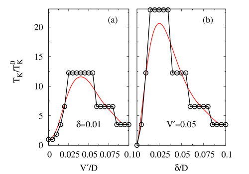
Figure 4: (color online) (a) Kondo temperature as function of $V^{\prime}$ for $\delta=0.01$. Notice $T_{K}$ at $V^{\prime}=0$ is non-zero, $T_{K}^{0}=5.6\times 10^{-5}$ here. (b) Kondo temperature as function of $\delta$ for $V^{\prime}=0.05$. Other parameters are as in Fig. 3. Notice $T_{K}\rightarrow 0$ for $\delta\rightarrow 0$. The step structure seen here results from the NRG discretization of the energy, and corresponds also to the discrete temperature values for which we calculate the thermodynamics (see below). Continuous lines show smooth fit of NRG results as guide to the eye.

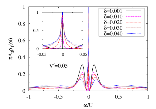
Figure 5: (color online) Spectral function vs. energy for $V=0.1$, $V^{\prime}=0.05$ and $\delta=0.04$ (short-dash, blue), $\delta=0.03$ (dotted, brown), $\delta=0.02$ (dashed, red), $\delta=0.01$ (dot-dash, magenta) and $\delta=0.001$ (solid, black). The inset shows a zoom of the region around $\omega=0$.

The zero-energy resonance also depends strongly on $\delta$. Figure 5 shows $\rho_{1}(\omega)$ for $V^{\prime}=0.05$ and several values of $\delta$. Notice that all curves show well-defined peaks and their positions remain nearly constant at either $\omega\approx 0$ or $\omega\approx\pm\sqrt{2{V^{\prime}}^{2}+\delta^{2}}$. However, the dips between the Kondo and the satellite peaks are less pronounced for larger $\delta$, and their position shifts with $\delta$, as can also be seen in the inset. The displacement of the dips toward the Fermi level as $\delta$ decreases produces a “squeezing” of the Kondo peak at the Fermi energy. The most evident situation shown in Fig.  5 is the case of $\delta=0.001$, when the Kondo resonance takes the form of a narrow and sharp peak. The behavior of $T_{K}$ with $\delta$ is shown in Fig.  4(b), and it is clearly non-monotonic as well. Notice that for $V^{\prime}=0.$05 we find a maximum value of $T_{K}\simeq 20T_{K}^{0}$ at $\delta\approx 0.025$. More importantly, the “squeezing” of the Kondo resonance as $\delta\rightarrow 0$ is accompanied by a strong suppression of $T_{K}$, which vanishes completely as $\delta\rightarrow 0$. The above behavior is a clear signal of the influence of the subtunneling mode on the Kondo state. Indeed, one can understand these results in terms of the Dicke state physics. For small values of $\delta$, the subtunneling Dicke state dominates and the Kondo temperature decreases. For sufficiently large values of $\delta$ the supertunneling Dicke state dominates and the Kondo temperature reaches its maximum value. For larger $\delta$ values, however, the system goes out of the Dicke regime and the Kondo temperature drops. Trocha We should also comment that the total suppression of the Kondo screening for $\delta=0$ is essentially a quantum phase transition, which results in the QD cluster isolating itself from the current leads. Perhaps one way to view this suppression of Kondo screening is to think of a Kondo resonance in the central dot that interferes destructively with the single-particle–like resonances of the side-connected dots (themselves hybridized with the leads via the central dot). The fact that all these resonances appear at the same energy, $\omega=0$, results in the eventual suppression of the Kondo state for the entire cluster. Of course, this is only a qualitative argument, ultimately validated by the NRG results. The underlying physical mechanism for this destructive interference and resulting ground state is fascinating, as we proceed to describe.

To provide a different perspective on the suppression of the Kondo screening (and vanishing Kondo temperature), we study the thermodynamical properties of the system, namely the contribution of the impurity to the magnetic moment, $\mu^{2}$, and the entropy, $S$, from which one extracts information about the nature of the states the system visits when the parameters are varied. As usual, $\mu^{2}(T)=\mu_{tot}^{2}(T)-\mu^{2}_{0}(T)$ and $S(T)=S_{tot}(T)-S_{0}(T)$, where $X_{tot}(T)$ and $X_{0}(T)$ (with $X=\mu^{2},S$) are thermodynamical quantities of the system calculated with and without impurity, respectively. The magnetic moment and the entropy can be written in terms of the magnetic susceptibility and the partition function as $\mu^{2}(T)=T\chi(T)$, and $S=\log Z$ (we set $k_{B}=1$). In order to study the effects of all three dots, we employ here the “cluster impurity” approach described in Sec. II.3.

Figures 6(a) and 7(a) show, respectively, $\mu^{2}$ and $S$ as function of the NRG iteration energy (temperature $T$) for several values of $V^{\prime}$ and $\delta$. Before engaging in the discussion of the more complicated situations, lets us examine the result for $V^{\prime}=\delta=0$ (small open circles, purple), corresponding to a single impurity case, as QD2 and QD3 have their level at the Fermi energy ($\delta=0$) but are decoupled from the rest of the system ($V^{\prime}=0$)–we include this curve as a reference for the more general cases. For $T\gg U$, all the curves show convergence to $\mu^{2}=3/8$ and $S=\log(64)$, resulting from the free orbital (FO) fixed point of the system. As $T\rightarrow 0$, DQ1 undergoes a crossover into a Kondo singlet state and its magnetic moment is screened by the conduction band, while QD2 and QD3 remain in their free orbital states (since $V^{\prime}=0$ and $\delta=0$), resulting in a net unscreened magnetic moment of $1/4$ and entropy $S=\log(16)$ for the three-dot cluster.

For $V^{\prime},\delta\neq 0$, different regimes can be found. In the low temperature limit ($T<T_{K}$) the system always flows into a Kondo state, where QD1 is in a Kondo singlet configuration with the reservoirs, while QD2 and QD3 are combined into a symmetric/antisymmetric pair of states, one of which is doubly occupied (and the other empty) at $T=0$, as schematically shown in Fig. 8(a). This situation is characterized by a magnetic moment completely screened by the conduction band ($\mu^{2}=0$) and with entropy $S=0$, as shown by all curves in Fig. 6 and 7.

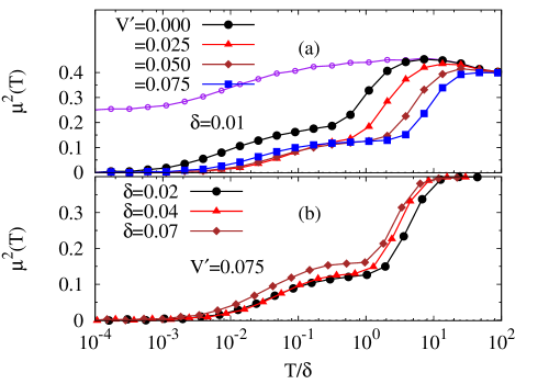
Figure 6: (color online) (a) Magnetic moment for the three-dot cluster as function of temperature for $\delta=0.01$ and various values of $V^{\prime}$. Open small circles (purple) show results for $V^{\prime}=\delta=0$. (b) Magnetic moment as function of temperature for $V^{\prime}=0.075$ and various values of $\delta$.

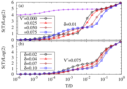
Figure 7: (color online) (a) Entropy of three-dot cluster as function of temperature for $\delta=0.01$ and various values of $V^{\prime}$. Open small circles (purple) show results for $V^{\prime}=\delta=0$. (b) Entropy of cluster as function of temperature for $V^{\prime}=0.075$ and various values of $\delta$.

Other interesting situations occur when $T_{K}<T<\delta$. T_K For $V^{\prime}\lesssim\delta$, the physics can still be understood in terms of the local orbitals, in which case (since $T<\delta$) QD2 and QD3 are still locked in one doubly-occupied and one empty state. In contrast, QD1 is in the magnetic moment regime, contributing alone to the magnetic moment $\mu^{2}=1/8$ and to the entropy $S=\log(2)$. When $V^{\prime}>\delta$, however, the system goes into a more intricate configuration of local molecular orbitals. This is better understood in terms of symmetric (super-tunneling) and anti-symmetric (sub-tunneling) combination of the QD2 and QD3 local orbitals, defined as

$$c_{+\sigma} = \frac{1}{\sqrt{2}}(c_{2\sigma}+c_{3\sigma})$$

$$c_{-\sigma} = \frac{1}{\sqrt{2}}(c_{2\sigma}-c_{3\sigma}),$$ (13)

where $c_{+\sigma}$ and $c_{-\sigma}$ annihilate an electron in the bonding and anti-bonding orbital, respectively, with energy $\varepsilon_{+}=\varepsilon_{-}=0$ (for $\varepsilon_{3}=-\varepsilon_{2}=\delta$ as before). With this transformation, the Hamiltonian of the dots reads

$$\tilde{H}_{dots} = \sum_{\sigma}\varepsilon_{1}c^{\dagger}_{1\sigma}c_{1\sigma}+Un_{1\uparrow}n_{1\downarrow}$$ (14)

$$+\sqrt{2}V^{\prime}\sum_{\sigma}\left[c^{\dagger}_{1\sigma}c_{+\sigma}+h.c.\right]$$

$$-\delta\sum_{\sigma}\left[c^{\dagger}_{+\sigma}c_{-\sigma}+h.c.\right].$$

The transformed system is schematically represented in Fig. 8(b). Note that the orbital “$+$” and “$-$” are coupled to each other by a matrix element $-\delta$ and only the orbital “$+$” couples to the QD1 via matrix element $\sqrt{2}V^{\prime}$. On this transformed basis we can provide a more intuitive analysis of the thermodynamic quantities as follows. For $T_{K}<T<\delta$ and $V^{\prime}\gg\delta$ the configuration of the system is represented in Fig. 8(c), where the QD1 orbital couples to the “$+$” orbital to form a “local singlet” (essentially decoupled from the leads), while the “$-$” orbital remains almost free (since $\delta\ll V^{\prime}$). The contribution to the magnetic moment and entropy is then provided solely by the “$-$” orbital, resulting in $\mu^{2}=1/8$ and $S=\log(4)$, as clearly seen in the curves with (blue) square symbols in Fig. 6(a) and 7(a). We should notice that the two curves for $V^{\prime}=0$ (for $\delta=0$ and $\delta=0.01$)–in each of the (a) panels of both figures–are identical for temperatures $T\gg\delta=0.01$, since for high $T$ the QD2 and QD3 levels at $\pm\delta$ are thermally accessible (which is no longer the case when $T\ll\delta$).

In Fig. 6(b) and 7(b) we fix $V^{\prime}=0.075$ and plot the magnetic moment and entropy for different values of $\delta$. For $\delta=0.02\ll V^{\prime}$, the situation described above is favored, but when $\delta\rightarrow V^{\prime}$, the plateaus in the susceptibility and entropy shift towards the curves with empty (black) circles of panel (a) in the respective figures. The system is then returning to the situation when the local orbitals are described independently, as shown in Fig. 8(d). Notice the Kondo singlet is not yet formed at these high temperatures ($T>T_{K}$).

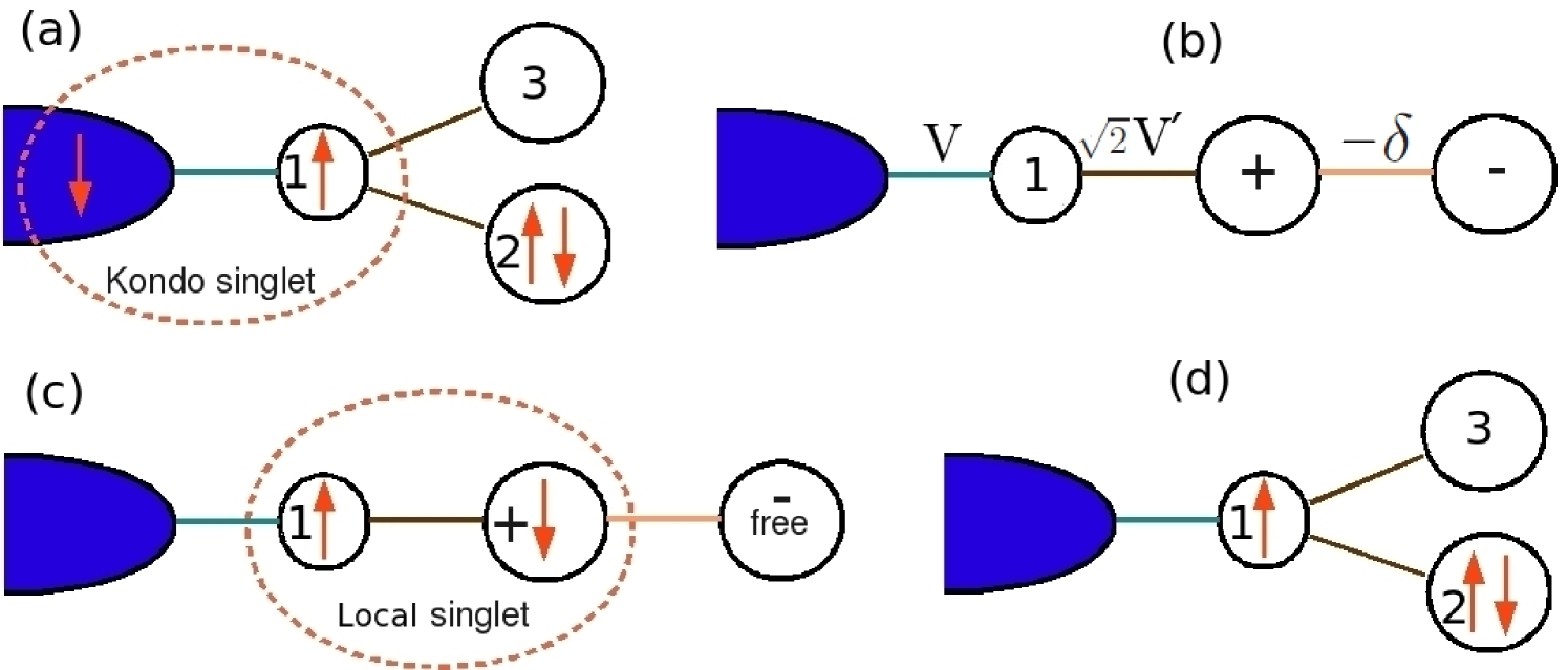
Figure 8: (color online) Schematic representation of the various configuration of the systems. (a) Kondo singlet for $\delta\neq 0$ and $T<T_{K}$. (b) Symmetric (“$+$”) and anti-symmetric orbital (“$-$”) combination. (c) Antiferromagnetic singlet formation between $\varepsilon_{1}$ and “$+$” orbital. (d) Magnetic moment configuration for $\delta\neq 0$ and $T>T_{K}$.

These results reveal the establishment of a local antiferromagneticaly correlated state, involving orbitals $\varepsilon_{1}$ and “$+$”, emerging at temperatures above $T_{K}$.

In order to provide more evidence of the local singlet between QD1 and the “$+$” orbital, Fig. 9 depicts the spin-spin correlation value $\langle{\bf S_{1}}\cdot{\bf S_{+}}\rangle$ (top panel); the correlation with the “$-$” orbital, $\langle{\bf S_{1}}\cdot{\bf S_{-}}\rangle$ is shown in the bottom panel, as function of temperature for various values of $V^{\prime}$. Notice that $\langle{\bf S_{1}}\cdot{\bf S_{+}}\rangle$ is always negative (antiferromagnetic) and has increasingly negative values for larger $V^{\prime}$. In contrast, the correlation between the spin in QD1 and in the “$-$” orbital is an order of magnitude weaker, and totally vanishes for large $V^{\prime}$. It is interesting to notice that although the local correlation with the “$+$” orbital is large, it does not fully exhaust the anticipated singlet correlation of $-3/4$, even for the larger $V^{\prime}$ values, where it seems to saturate at $\simeq-1/2$.

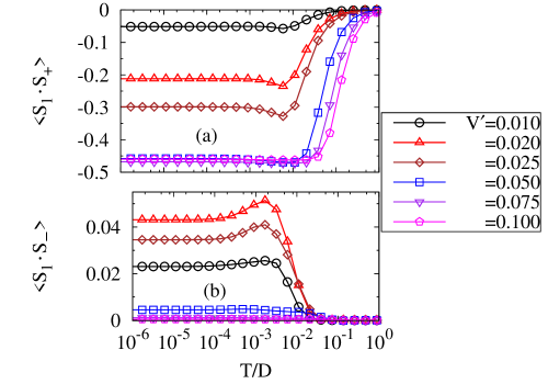
Figure 9: (color online) Spin-spin correlations as function of $T$ for $\delta=0.01$ and various values of $V^{\prime}$. Lower panel proves that the spin correlation of QD1 with “$-$” is vanishingly small. In contrast, upper panel exhibits strong antiferromagnetic correlation with the “$+$” orbital with increasing $V^{\prime}$.

III.2 Effects of particle-hole asymmetry

In a typical experimental situation, asymmetry in the structure parameters is more likely to occur. It is therefore of interest to analyze the stability and behavior of the results discussed above with respect to changes that more generally make the problem particle-hole asymmetric. We introduce asymmetry parameters $\kappa_{v}$ and $\kappa_{\delta}$ that allow for $V_{12}\neq V_{13}$, and $|\epsilon_{3}|\neq|\epsilon_{2}|$, respectively as:

$$V_{1l}=V^{\prime}(1\pm\kappa_{v})$$ (15)

and

$$\epsilon_{l}=\delta(1\pm\kappa_{\delta}),$$ (16)

where the positive (negative) sign in the expressions above corresponds to the index $l=2~{}(3)$. The fully symmetric situation previously described corresponds obviously to the case $\kappa_{v}=\kappa_{\delta}=0$.

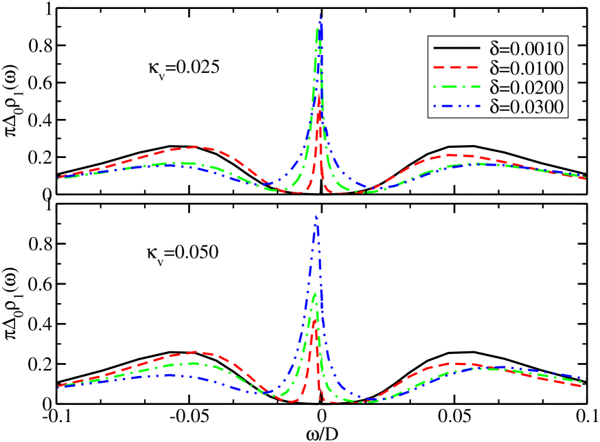
Figure 10: (color online) Spectral function vs. energy for asymmetric coupling to the side dots. Top panel ($\kappa_{v}=0.025$) and bottom panel ($\kappa_{\delta}=0.05$) $V=0.1$, $V^{\prime}=0.05$ and $\delta=0.001$ (solid, black), $\delta=0.01$ (dashed, red), $\delta=0.02$ (dot-dash, green), and $\delta=0.03$ (dot-dot-dash, blue).

We first allow for asymmetry in the couplings to the side dots; Fig. 10 shows the results for weakly asymmetric couplings $V_{12}$ and $V_{13}$ for different values of $\delta$. The top (bottom) panel shows the case of $\kappa_{v}=0.025$ ($\kappa_{v}=0.05$). The asymmetry in the couplings results in a shift of the central peak away from the Fermi level, as well as its strong suppression (compare with Fig. 5). This effect is less pronounced for larger values of $\delta$. Notice, for instance, that for $\delta=0.001$ the central peak is almost completely suppressed. Also, comparing the curves in the top and bottom panels, we observe that for a given $\delta$ the shift and suppression of the peak is larger as $\kappa_{v}$ increases.

In Fig. 11 we fix $\delta=0.01$ and $\kappa_{v}=0$ (symmetric couplings to central dot), and show the spectral function as function of energy for two values of $\kappa_{\delta}$ and different values of $V^{\prime}$. In the top (bottom) panel we have $\kappa_{\delta}=0.025$ ($\kappa_{\delta}=0.05$). We notice that for small $V^{\prime}$ (for instance $V^{\prime}=0.01$), there is a strong distortion in the spectral function near the Fermi level for both values of $\kappa_{\delta}$. However this distortion is much weaker when $V^{\prime}$ increases, so that for $V^{\prime}=0.02$ and $0.03$, the asymmetry in the spectral function is nearly absent.

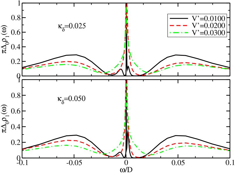
Figure 11: (color online) Spectral function vs. energy for the asymmetric bare levels about the Fermi level, with asymmetries $\kappa_{\delta}=0.025$ (top) and $\kappa_{\delta}=0.050$ (bottom). The other parameters are $V=0.1$, $\delta=0.01$ and $V^{\prime}=0.01$ (solid, black), $V^{\prime}=0.02$ (dashed, red), and $V^{\prime}=0.03$ (dot-dash, green).

One would expect, from seeing these results for the spectral functions, that the particle-hole asymmetry in the system would introduce non-monotonic changes in the Kondo temperature. In Fig. 12 we illustrate this point. Panel (b) shows the associated Kondo temperature for the system parameters of Fig. 10a, where the coupling to the side dots is asymmetric (with a value of $\kappa_{v}=0.025$). As suggested by the increasing width of the zero-energy peak in Fig. 10a, $T_{K}$ increases with $\delta$, reestablishing the Kondo state that was absent in the full Dicke regime (for $\delta=0$), while larger values eventually reduce $T_{K}$, although not to zero. Similarly, the asymmetry in side dot level location illustrated in Fig. 11a, results in a rapid increase of $T_{K}$ with $V^{\prime}$, shown in panel (a), so that the system has an order of magnitude larger Kondo temperature for $V^{\prime}\approx 0.05$, before dropping for larger $V^{\prime}$ values.

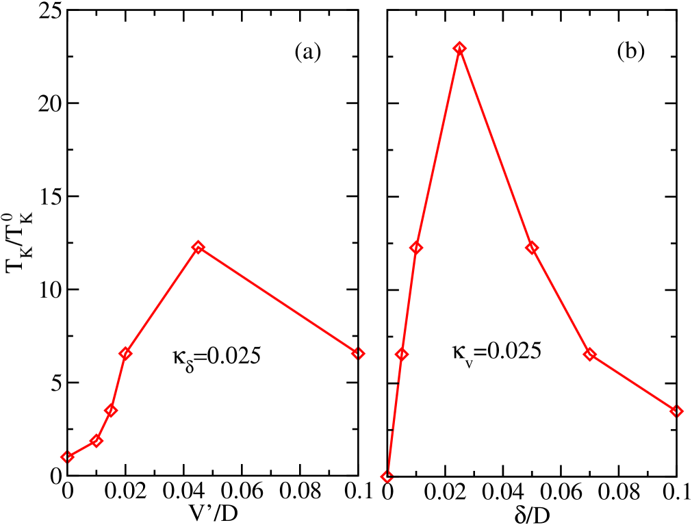
Figure 12: (color online) Kondo temperature for asymmetric three-dot systems. Panel (a) shows $T_{K}$ (in units of $T_{K}^{0}$ – see caption Fig. 4) for system of Fig. 11a. Panel (b) shows $T_{K}$ for system of Fig. 10a. Notice strong enhancement of $T_{K}$ in both cases with increasing parameter.

An additional important source of particle-hole asymmetry is the bare level position of QD1. In order to explore how it affects our results, we allow the level $\epsilon_{1}$ to be different from $-U/2$. For convenience, we keep $\epsilon_{1}=-0.25$ and change $U$, which allows not only to explore the effect of the particle-hole asymmetry but also the effect of larger values of $U$. Figure 13 shows the spectral function vs. energy for $\delta=0.01$ and various values of $U$. The curve for $U=0.5$, corresponding to the symmetric case studied in Sec. III.1, exhibits two peaks symmetrically placed about the Fermi level, as well as Hubbard bands located near $\epsilon_{1}$ and $\epsilon_{1}+U$, as can be seen in the inset of the figure. As $U$ increases, one clearly observes that the curves no longer display particle-hole symmetry. We observe a decreasing height of the central peak, as well as a minor shift in position, while its width remains almost unchanged with increasing $U$. More interesting, we notice that the satellite peak below the Fermi level is suppressed and shifted toward $\omega=0$, while the corresponding peak on the positive side is nearly unchanged. This is a clear consequence of breaking particle-hole symmetry in the problem.

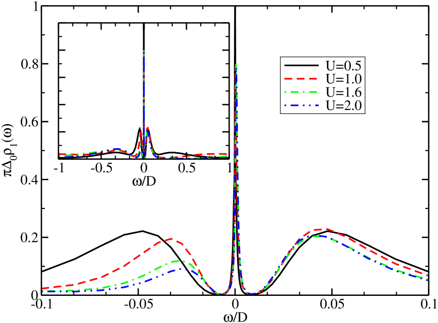
Figure 13: (color online) Spectral function vs. energy for $V=0.1$, $V^{\prime}=0.05$, $\delta=0.01$ and $U=0.5$ (solid, black), $U=1.0$ (dashed, red), $U=1.6$ (dot-dash, green), and $U=2.0$ (dot-dot-dash, blue) (solid, black). The inset shows the same curves for the entire region within the conduction band.

We have also investigated the role of non-vanishing Coulomb interactions in the side dots QD2 and QD3. To that effect, the problem is addressed using NRG for the three quantum dot complex treated as a cluster impurity, as described in Sec. II.3, and with the inclusion of a non-zero Coulomb interaction $U_{2}=U_{3}=U^{\prime}$. Figure 14 presents the spectral function for different values of $U^{\prime}$, for QD2 and QD3 levels placed asymmetrically about the Fermi level ($\delta=0.01$). For $U^{\prime}=0$ the system is particle-hole symmetric (as $\varepsilon_{1}=-U/2$), as also shown in Fig. 3. For increasing $U^{\prime}$, however, the asymmetry in the spectral function is evident, strongly shifting and suppressing the Kondo resonance near the Fermi level. This indicates the important role that Coulomb interactions in the nearby dots have in the overall correlations present in the system, and suggests that the observation of the Dicke effect is indeed a delicate undertaking.

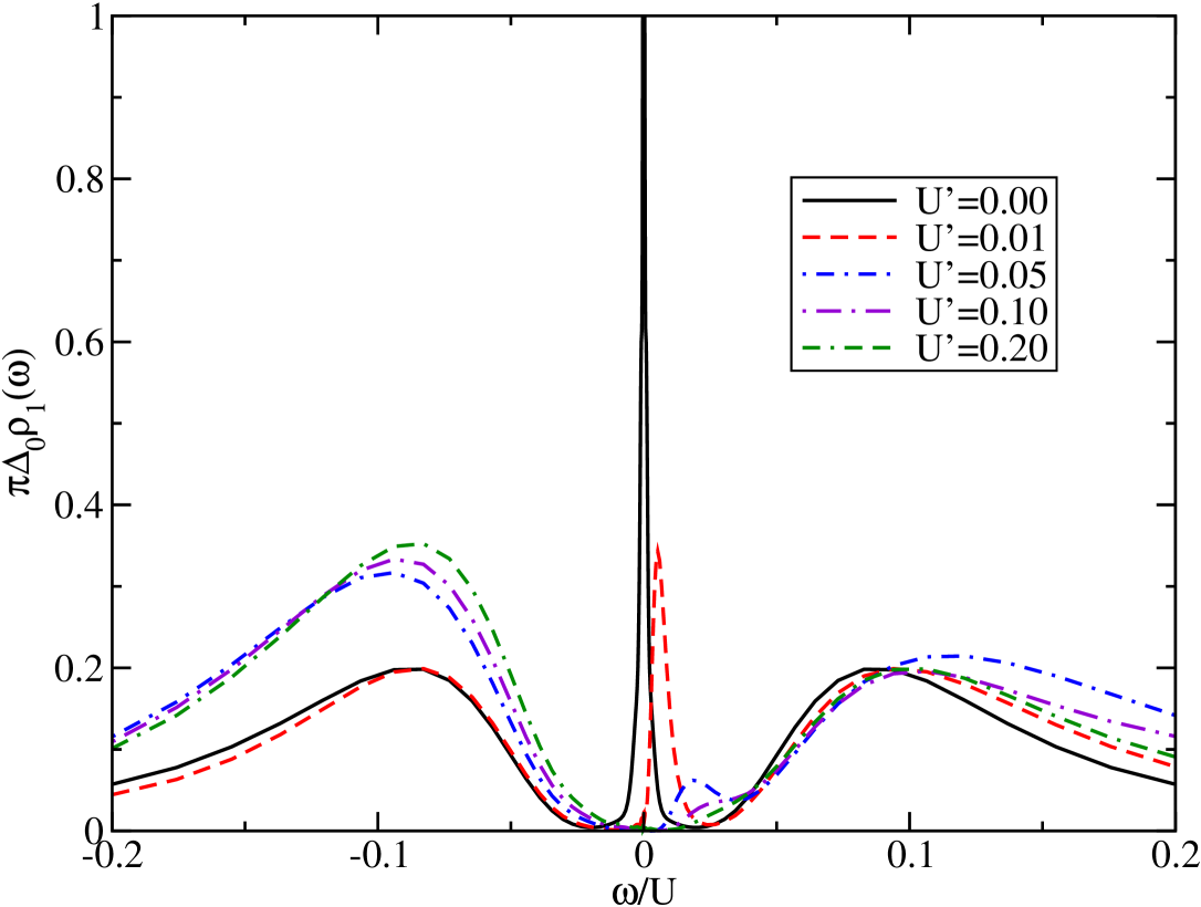
Figure 14: (color online) Spectral function for the three dot cluster with non-zero Coulomb interaction in all dots for energies close to the Fermi level. The solid (black) curve with $U^{\prime}=0$ represents the same system as in Fig. 3, $\delta=0.01$, $V^{\prime}=0.05$, $V=0.1$, and $U=0.5$. As $U^{\prime}$ increases, the asymmetry is evident, strongly affecting the Kondo peak near zero energy.

III.3 Conductance

We now turn our attention to the effect on the conductance of the system of the various features discussed above. It is clear that the details of the density of states at the Fermi level are directly connected to the zero-temperature transport properties in linear response. In the zero-bias limit, the conductance of the system can be obtained by the Landauer formula, $G=(2e^{2}/h)\int_{-\infty}^{\infty}-{\tt Im}[{\cal T}(\omega)]\left(\partial f(\omega)/\partial\omega\right)d\omega$, where $f(\omega)$ is the Fermi distribution function and, in the present case, ${\cal T}(\omega)=\Delta_{0}G_{dd}(\omega)$. At $T=0$ the conductance reduces to $G=(2e^{2}/h)\pi\Delta_{0}\rho_{1}(E_{F})$. From the density of states in Fig. 3 and 5 we observe that for all values of $V^{\prime}$ and $\delta>0$, the DOS always exhibits a Kondo peak at the Fermi level (which becomes very narrow and sharp as $\delta\rightarrow 0$). Since the conductance of the system is proportional to the density of states of DQ1, this results in unitary conductance ($2e^{2}/h$) for all values of $V^{\prime}$ and $\delta>0$, discontinuously dropping to zero at $\delta=0$. The above behavior is explained by the complete localization of the subtunneling state for $\delta=0$. In this case the state has no projection on the central quantum dot and therefore it does not contribute to the conduction. Similarly, one would expect vanishing conductance for small bias as long as $\delta=0$. Trocha

An interesting result of the particle-hole asymmetry, as we have seen in the previous section, is to shift the Kondo resonance away from the Fermi level, as well as to change its amplitude. This has direct impact on the linear conductance of the structure. Figure 15 illustrates this behavior for different asymmetries (notice in fact that although $\kappa_{v}$ and $\kappa_{\delta}$ are constant in this figure, increasing $V^{\prime}$ or $\delta$ value increases the asymmetry of the structure). In both cases, the conductance is indeed found to change drastically with the appropriate parameter. It is interesting that asymmetry in the QD2 and QD3 level position (for $\kappa_{\delta}=0.025$) and increasing dot coupling $V^{\prime}$ results in a strong suppression of the linear conductance, even as the Kondo temperature of the system (Fig. 12a) is increasing. On the other hand, the enhancement of $T_{K}$ that we see for the coupling asymmetry ($\kappa_{v}=0.025$) in Fig. 12b, does produce a rapid increase in conductance for larger $\delta$ values.

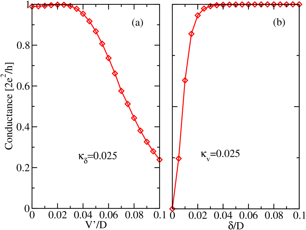
Figure 15: (color online) Conductance for asymmetric systems corresponding to Fig. 12, for each of the two panels there.

IV Conclusions

In summary, we have investigated the interplay of Dicke and Kondo effects in a central strongly interacting quantum dot coupled to a conduction band and two localized levels provided by additional nearly non-interacting dots. We study in detail the Kondo regime of the system, by applying a numerical renormalization group analysis to a finite-$U$ multi-impurity Anderson Hamiltonian model. We find that the system displays a “squeezed” Kondo resonance as we tune the single particle levels of the side-coupled dots toward the Fermi level. In the strict Dicke limit of degenerate single-particle levels, the Kondo singlet disappears, as its Kondo temperature vanishes. This behavior is found to be closely related to the formation of a local singlet state involving the (coupled) orbitals of the interacting dot and the super-tunneling state (the symmetric combination of the single particle levels of the two side coupled dots). This local singlet results in the suppression of the Kondo screening, which is detrimental to the conductance of the system. We have further explored the consequences of system asymmetries, introduced by different couplings, level locations and Coulomb interactions. These are found to strongly affect the spectral density and the conductance through the structure. We believe that our study not only clarifies the relevant picture of an interacting system coupled to side quantum dots and conduction band, but it also provides important guidelines for experimental realization of these ideas.

V Acknowledgements

We thank helpful discussions with N. Sandler and G. B. Martins and financial support from CNPq, CAPES, FAPEMIG, NSF-PIRE, and MWN/CIAM (CNPq, CONICYT, NSF-DMR). P.A.O acknowledges financial support from CONICYT/Programa Bicentenario de Ciencia y Tecnologia (CENAVA, grant ACT27) and FONDECYT, under grant 1080660.

References

- (1) D. Goldhaber-Gordon, H. Shtrikman, D. Mahalu, D. Abusch-Magder, U. Meirav, and M. A. Kastner, Nature 391, 156 (1998).
- (2) T. Inoshita, Science 281, 526 (1998).
- (3) S. M. Cronenwett, T. H. Oosterkamp, and L. P. Kouwenhoven, Science 281, 540 (1998).
- (4) S. Sasaki et al., Nature 405, 764 (2000).
- (5) M. Putilsnik and L. I. Glazman, Phys. Rev. Lett. 87, 216601 (2001)
- (6) C. A. Büsser et al, Phys. Rev. B 62, 9907 (2000).
- (7) H. Jeong, A. M. Chang, M. .R. Melloch, Science 293, 2221 (2001).
- (8) P. S. Cornaglia, D. R. Grempel, Phys. Rev. B 71, 075305 (2005).
- (9) E. Vernek, N. Sandler, S. E. Ulloa, and E. V. Anda, Phys. E 34, 608 (2006).
- (10) L. G. G. V. D. Dias da Silva, N. Sandler, K. Ingersent, and S. E. Ulloa, Phys. Rev. Lett. 97, 096603 (2006); L. G. G. V. D. Dias da Silva, N. Sandler, P. Simon K. Ingersent, and S. E. Ulloa, Phys. Rev. Lett. 102, 166806 (2009).
- (11) S. Sasaki, H. Tamura, T. Akazaki, and T. Fujisawa, Phys. Rev Lett. 103, 266806 (2009).
- (12) R. Žitko, arXiv:1001.1983v2 [cond-mat.mes-hall].
- (13) T. Kuzmenko, K. Kikoin, Y. Avishai, Europhys. Lett. 64, 218 (2003).
- (14) Z. T. Jiang, Q. F. Sun, and Y. P. Wang, Phys. Rev. B 72, 045332 (2005).
- (15) R. Žitko and J. Bonča, A. Ramšak, and T. Rejec, Phys. Rev. B 73, 153307 (2006).
- (16) A. M. Lobos, and A. A. Aligia, Phys. Rev. B 74, 165417 (2006).
- (17) E. Vernek, C. A. Büsser, G. B. Martins, E. V. Anda, N. Sandler, and S. E. Ulloa, Phys. Rev. B 80, 035119 (2009).
- (18) T. Numata, Y. Nisikawa, A. Oguri, and A. C. Hewson, Phys. Rev. B 80, 155330 (2009).
- (19) G. Chiappe, E. V. Anda, L. Costa Ribeiro, and E. Louis, Phys. Rev. B 81, 041310 (2010).
- (20) R. Leturcq, L. Schmid, K. Ensslin, Y. Meir, D. C. Driscoll, and A. C. Gossard, Phys. Rev. Lett. 95, 126603 (2005).
- (21) M. C. Rogge and R. J. Haug Phys. Rev. B 77, 193306 (2008).
- (22) U. Fano, Phys. Rev. 124, 1866 (1961).
- (23) W. Hofstetter, J. Konig, and H. Schoeller, Phys. Rev. Lett. 87, 156803 (2001).
- (24) E. Vernek, N. Sandler, and S. E. Ulloa, Phys. Rev. B 80, 041302(R) (2009).
- (25) M. Sato, H. Aikawa, K. Kobayashi, S. Katsumoto, and Y. Iye, Phys. Rev. Lett. 95, 066801 (2005).
- (26) D. Withoff and E. Fradkin, Phys. Rev. Lett. 64, 1835 (1990).
- (27) K. Ingersent, Phys. Rev. B 54, 11936 (1996); C. Gonzalez-Buxton and K. Ingersent, Phys. Rev. B 57, 14254 (1998).
- (28) P. A. Orellana, G.A. Lara, and E. V. Anda, Phys. Rev. B 74, 193315 (2006).
- (29) R. H. Dicke, Phys. Rev. 89, 472 (1953).
- (30) T. V. Shahbazyan and S. E. Ulloa, Phys. Rev. Lett. 79, 3478(1997); Phys. Rev. B 57, 6642 (1998).
- (31) A. L. Chudnovskiy, and S. E. Ulloa, Phys. Rev. B 63, 165316 (2001).
- (32) T. Brandes, Phys. Rep. 408, 315 (2005).
- (33) P. Debray, O. E. Raichev, P. Vasilopoulos, M. Rahman, R. Perrin, W. C. Mitchell, Phys. Rev. B 61 10950 (2000).
- (34) M. E. Torio, K. Hallberg, A. H. Ceccatto, C. R. Proetto, Phys. Rev. B 65, 085302 (2002).
- (35) P. Trocha and J. Barnaś, Phys. Rev. B 78, 075424 (2008).
- (36) K. Wilson, Rev. Mod. Phys. 47 773 (1975).
- (37) H. R. Krishna-murthy, J. W. Wilkins, and K. Wilson, Phys. Rev. B 21, 1003 (1980); H. R. Krishna-murthy, J. W. Wilkins, and K. Wilson, Phys. Rev. B 21, 1044 (1980).
- (38) R. Bulla, T. A. Costi, and T. Pruschke, Rev. Mod. Phys. 80, 395 (2008).
- (39) K. Chen and C. Jayaprakash, Phys. Rev. B 20, 14436 (1995).
- (40) L. A. Fetter and J. D. Walecka, Quantum Theory of Many-Particle Systems (Dover, New York, 2003).
- (41) R. Bulla, T. A. Costi, and D. Vollhardt, Phys. Rev. B 64, 045103 (2001).
- (42) . We typically keep 1200 states in the NRG runs and use a discretization parameter .
- (43) The Kondo temperature is obtained using Wilson’s criterion, e.g., .