Plasticity and reversibility of structural transitions in a model solid

Abstract

We formulate a phenomenological elasto-plastic theory to describe a solid undergoing a structural transition from a square ($p4mm$) to an oblique ($p2$) lattice in two dimensions. Within our theory, the components of the strain may be decomposed additively into separate elastic and plastic contributions. The plastic strain, produced when the local stress crosses a threshold, is governed by a phenomenological equation of motion. We investigate the dynamics of shape of an initially square solid as it is cycled through a transformation protocol consisting of (1) a quench across the transition (2) deformation by an external stress and finally (3) reverse transformation back to the parent state. We show that shape recovery at the end of this cycle depends on crucially on the presence of plasticity in components of the strain responsible for the transformation.

I Introduction

The question of the degree and efficiency of shape reversibility of solids undergoing reversible Martensitic transitionspaper0 is clearly of considerable technological importance considering the diverse applications of shape memory or “smart” materialssmm .

The necessary criterion for a material in order to exhibit shape-memory is that the symmetry group of the product phase forms a sub-group of the parent and the transformation leads to symmetry breakingkaushik . In a recent publication we had explored the possible sufficient conditions for shape reversibility using a model system in two dimensions as a test casenanomart . In our model system it was possible to influence the nature of the transformation by tuning the parameters of the interaction potentialpaper1 . We found that, while a square ($p4mm$) to a rhombic (in general, oblique - $p2$) lattice was reversiblehatch , the transformation to the more symmetric, triangular ($p6$) lattice was not, in accordance with the conclusions of Ref.kaushik . However, we found that the question of reversibility was linked to the extent and nature of plastic or non-affine zones (NAZs) present within the transforming crystal. The positions of particles which belong to the NAZs cannot be obtained from a simple affine (shear and/or scaling) transformation of the parent lattice. We identified two kinds of NAZs associated either with the non-order parameter (NOP) (e.g. volumetric) strain or with the order-paramter (OP) shear strain which transforms the square to a rhombic lattice. We argued that the $p4mm\leftrightharpoons p2$ produces only NAZs of the first kind while during a $p6\to p4mm$ transition, we gave indirect evidence that both kinds of NAZs are likely to be produced leading to irreversibility. We concluded therefore that for reversibility it is sufficient that NAZs associated with OP strains not be produced. To support our claim, we showed that eliminating NAZs by making the solid stronger or the system size smaller than the typical distance between NAZs makes even the $p4\to p6$ transformation reversible in apparent contradiction to Ref.kaushik .

In this paper, we lend further support to this claim by investigating this problem from the point of view of a phenomenological elasto-plastic theorypaper2 of the square to oblique transformation. The elasto-plastic theory has been shown earlier to reproduce the qualitative features of the results of our MD simulationspaper1 . One of the advantages of this approach is that plasticity in the NOP or the OP sector may be introduced systematically and their effects observed explicitly.

Our main results are as follows. We study the reversibility of shape of a solid which is first quenched from a square into the rhombic phase, deformed by an external stress and finally brought back to the square phase (see Fig.1). The external control parameters are the temperature and stress. We compare the initial and final shapes of the solid and look for congruence. We show that the presence of plasticity exclusively in the NOP sector does not affect shape reversibility while the presence of plasticity in the OP sector triggers irreversibility in shape changes.

The next section is dedicated to a quick review of our elasto-plastic theory where we discuss the formalism and how to deduce shape at each instant of time from the knowledge of strains at that instant. In section III we present our results and we conclude in section IV indicating possible future directions.

II Elasto-plastic theory

In this section we formulate our elasto-plastic continuum theory for structural transitions in solids. Our theory allows us to determine the microstructure and the overall shape of a solid undergoing a square to a general oblique lattice. Unlike previous work in this subjectstrn-only we allow for the presence of non-affine, or plastic deformationspaper1 ; paper2 .

Our main assumption in what follows is that the components of the strain tensorLandau may be additively decomposed into elastic (affine) and plastic partselastop , viz. $e_{ij}=e_{ij}^{A}+e_{ij}^{P}$ where $i,j=x,y$. The plastic strains $e_{ij}^{P}$ represents the total contribution from, in general, space and time dependent defect fields, which, in the spirit of our continuum approach, need not be resolved into individual, microscopic defects. Nevertheless, defects introduce multivaluedness in the particle displacement field $\mathbf{u}=(u_{x}(\mathbf{r}),u_{y}(\mathbf{r}))$ and cause the elastic parts of the strain to violate the St. Venant’s compatibility conditionbaus ,

$$\nabla\times(\nabla\times\bar{\bar{e}}^{A})^{T}=-\nabla\times(\nabla\times\bar{\bar{e}}^{P})^{T}\neq 0,$$ (1)

where $\bar{\bar{e}}^{A}$ and $\bar{\bar{e}}^{P}$ represents the affine (elastic) and the plastic strain tensors respectively. Note that Eq.(1) implies that the total strain $e_{ij}$ does satisfy the compatibility condition.

The structural transition is driven by the non-linear response of the solid to one or more components of the strain- the order parameter (OP). For example, for the ($p4mm\to p2$) transition, the order parameter strains are $e_{2}=e_{xx}-e_{yy}$ and $e_{3}=e_{xy}=e_{yx}$ while the remaining volumetric strain $e_{1}=e_{xx}+e_{yy}$ is a non-order parameter (NOP) strainhatch . We shall first consider the case when plasticity exists only in the NOP sector.

The transition is described by the following free energy functional:

$${\cal F} = \frac{1}{2}\int\,{\rm dxdy}\,\left[a_{1}(e_{1}^{A})^{2}\,+\,a_{2}e_{2}^{2}\,+\,a_{3}e_{3}^{2}-b_{3}e_{3}^{4}+d_{3}e_{3}^{6}\right.$$

$$+ \left.\,c_{1}(\nabla e_{1}^{A})^{2}\,+\,c_{2}(\nabla e_{2})^{2}\,+\,c_{3}(\nabla e_{3})^{2}\right].$$

Note that in Eq.(II) we have made the simplifying assumption that the product oblique lattice is actually a rhombus so that the equilibrium value of $e_{2}=0$. This choice is motivated by our MD simulation of a particular model solid paper1 though we do not doubt that our theory may be easily extended to the general case. The three elastic constants $a_{1},a_{2}$ and $a_{3}$ define the linear elasticity of the square (parent) phase. The connection with external control parameters such as temperature ($T$) is, as usual, through the temperature dependence of these coefficients especially $a_{3}\propto(T-T^{*})/T^{*}$ where $T^{*}$ is the limit of stability of the square solid. Reducing $a_{3}$ by cooling the solid stabilizes the rhombic phase (see Fig. 1). The rest of the coefficients parametrize non-linearities and may be taken to be constants.

The Lagrangian is given bystrn-only ,

$${\cal L} = \int\frac{\rho}{2}\left[(\dot{u}_{x}^{2}+\dot{u}_{y}^{2})\right]dxdy-{\cal F}.$$ (3)

To obtain the equation of motion in the displacement fields, we need to solve the Euler Lagrange equation:

$$\frac{d}{dt}\frac{\partial L}{\partial\dot{u}_{i}}-\frac{\partial L}{\partial u_{i}}=-\frac{\partial R}{\partial\dot{u}_{i}}.$$ (4)

The Rayleigh dissipation functional Landau ${\cal R}$ is given by ${\cal R}=\frac{1}{2}\int\left[\xi(\dot{e}_{1}^{A})^{2}+\kappa\dot{e}_{2}^{2}+\gamma\dot{e}_{3}^{2}\right]dxdy$, where the coefficients $\xi,\kappa$ and $\gamma$ are the corresponding viscosity coefficients of the system.

Using Eqs.(II), (3) and (4), we obtain the following equations of motion for the affine strains $e_{1}^{A},e_{2}$ and $e_{3}$:

$$\rho\ddot{e}_{1}^{A} = \nabla^{2}\left(\frac{\delta{\cal F}}{\delta e_{1}^{A}}+\frac{\delta{\cal R}}{\delta\dot{e}_{1}^{A}}\right)+\frac{\partial^{2}}{\partial x\partial y}\left(\frac{\delta{\cal F}}{\delta e_{3}}+\frac{\delta{\cal R}}{\delta\dot{e}_{3}}\right)$$ (5)

$$+ {\cal W}^{2}\left(\frac{\delta{\cal F}}{\delta e_{2}}+\frac{\delta{\cal R}}{\delta\dot{e}_{2}}\right),$$

$$\rho\ddot{e}_{2} = \nabla^{2}\left(\frac{\delta{\cal F}}{\delta e_{2}}+\frac{\delta{\cal R}}{\delta\dot{e}_{2}}\right)+{\cal W}^{2}\left(\frac{\delta{\cal F}}{\delta e_{1}^{A}}+\frac{\delta{\cal R}}{\delta\dot{e}_{1}^{A}}\right),$$ (6)

$$\rho\ddot{e}_{3} = \frac{1}{4}\nabla^{2}\left(\frac{\delta{\cal F}}{\delta e_{3}}+\frac{\delta{\cal R}}{\delta\dot{e}_{3}}\right)+\frac{\partial^{2}}{\partial x\partial y}\left(\frac{\delta{\cal F}}{\delta e_{1}^{A}}+\frac{\delta{\cal R}}{\delta\dot{e}_{1}^{A}}\right).$$ (7)

where the “wave” operator ${\cal W}^{2}$ is defined as ${\cal W}^{2}=\partial^{2}/\partial x^{2}-\partial^{2}/\partial y^{2}$. Since there is symmetry breaking in the space of the OP strains, the dynamics of $e_{2}$ and $e_{3}$ – the broken symmetry variables – is much slower than that of the affine NOP strain $e_{1}^{A}$. Therefore $e_{1}^{A}$ reaches a steady state much faster compared to $e_{2}$ and $e_{3}$ and we can simplify Eqs.(5-6) by assuming that $e_{1}^{A}$ is slaved, at all times, to the OP strains $e_{2}$ and $e_{3}$. Also note that, the St. Venant’s compatibility condition, which in two dimensions can be explicitly written as

$$\nabla^{2}e_{1}-{\cal W}^{2}e_{2}-4\nabla_{x}\nabla_{y}e_{3}=0,$$ (8)

may be used to eliminate $e_{2}$ from Eqs.(5-6).

The final set of equations which therefore has to be solved to obtain the affine strains are

$$\nabla^{2}e_{1}^{A} = \left(\frac{4a_{2}-a_{3}}{a_{1}+a_{2}}\right)\frac{\partial^{2}e_{3}}{\partial x\partial y}-\left(\frac{a_{2}}{a_{1}+a_{2}}\right)\nabla^{2}e_{1}^{P}.$$ (9)

$$\rho\ddot{e}_{3} = \frac{1}{4}\nabla^{2}\left(a_{3}e_{3}-b_{3}e_{3}^{3}+d_{3}e_{3}^{5}-c_{3}\nabla^{2}e_{3}\right.$$ (10)

$$- \left.\ 4c_{1}\frac{\partial^{2}e_{1}^{A}}{\partial x\partial y}+\gamma\dot{e}_{3}\right)+\frac{\partial^{2}}{\partial x\partial y}\left(a_{1}e_{1}^{A}+\xi\dot{e}_{1}^{A}\right)$$

Figure 1: The homogeneous part of the free energy functional ${\cal F}(e_{3})$ as a function of the OP strain $e_{3}$ for different values of the parameters $a_{3}$ and the external stress $\sigma_{3}$ viz. $a_{3}=0.5,\sigma_{3}=0$ (I), $a_{3}=0.1,\sigma_{3}=0$ (II) and $a_{3}=0.1,\sigma_{3}=.1$ (III). The rest of the parameters $b_{3}=-1$ and $d_{3}=1$ throughout. Inset shows a schematic representation of the typical dynamics of plastic strain $\dot{e}_{i}^{P}$ as a function of the local stress $\sigma_{i}$ used in our calculations. Similar dynamics is assumed for volumetric (NOP, $i=1$) as well as shear (OP, $i=3$) plasticity. The threshold stress $\sigma_{ic}$ is, of course, different in the two cases.

Lastly, the dynamics of the plastic strain $e_{1}^{P}$ needs to be specified. We assume that this is given by the following simple phenomenological equation of motion used by us (Fig. 1 inset) is,

$$\dot{e}_{1}^{P} = \frac{1}{h_{1}}\,\,\,\sigma_{1}-c_{p}\nabla^{2}e_{1}^{P}\,\,\,\,\,\,\,\,\,\,\,\,\,\,\,\,\,\,\,{\rm if}\,|\sigma_{1}|>\sigma_{1c}$$

$$= -c_{p}\nabla^{2}e_{1}^{P}\,\,\,\,\,\,\,\,\,\,\,\,\,\,\,\,\,\,\,\,\,\,\,\,\,\,\,\,\,\,\,\,\,\,\,\,\,\,\,\,\,\,{\rm otherwise}$$

where the local volumetric stress $\sigma_{1}=\delta{\cal F}/\delta e_{1}^{A}$, and we have chosen a Newtonian ansatz with a simple threshold criterion with yield stress $\sigma_{1c}$ for simplicity. Note that Eq.II also includes strain diffusion.

The continuum elasto-plastic theory described above has been successfully used in the pastpaper2 to describe microstructure selection following a quench from the square to the oblique phase. For large values of $h_{1}$ in Eq.(II) $e_{1}^{P}$ is produced only at the parent-product interface within localized and transient NAZs. Once coarse-grained over distances large compared to the typical size of these NAZs, the twinned microstructure obtained in this limit become identical to that seen in “strain-only” approachesstrn-only which do not involve plasticity. On the other hand, for small values of $h_{1}$, $e_{1}^{P}$ proliferates the entire solid and effectively screen non-local elastic interactions, completely changing the microstructure from twinned martensite to un-twinned ferrite. In this limit the coarse- graining length grows to become of the order of the system size and such microstructures cannot be described within the earlier strain only theorystrn-only . These results closely mimic those observed in our MD simulations of the square $\leftrightharpoons$ oblique transformation in a model solidpaper1 .

In this paper we wish to study shape recovery following a quench- deform- reheat transformation cycle for a solid undergoing a structural transition in the presence of plasticity. We therefore need to include the effect of external stress by using a modified Lagrangian, namely,

$${\cal L}=\int\frac{\rho}{2}\left[(\dot{u}_{x}^{2}+\dot{u}_{y}^{2})\right]dxdy-{\cal F}+f_{x}u_{x}+f_{y}u_{y}$$ (12)

where $f_{x}$ and $f_{y}$ are the components of the tangential forces along the $x$ and $y$ direction respectively applied at the edges of the system. The dynamical equations for the affine strains, obtained from this Lagrangian are

$$\rho\ddot{e}_{3} = \frac{1}{4}\nabla^{2}\left(a_{3}e_{3}-b_{3}e_{3}^{3}+d_{3}e_{3}^{5}-c_{3}\nabla^{2}e_{3}\right.$$ (13)

$$- \left.\ 4c_{1}\frac{\partial^{2}e_{1}^{A}}{\partial x\partial y}+\gamma\dot{e}_{3}\right)+\frac{\partial^{2}}{\partial x\partial y}\left(a_{1}e_{1}^{A}+\xi\dot{e}_{1}^{A}\right)$$

$$+ \sigma_{3}$$

Note that, the external shear stress $\sigma_{3}=\frac{\partial f_{x}}{\partial y}+\frac{\partial f_{y}}{\partial x}$ does not affect the steady state equation for the affine NOP strain $e_{1}^{A}$. The phenomenological equation for the plastic strain also remains same as well.

If, in addition, plasticity is associated with the OP strain, $\sigma_{3}$ may also give rise to plastic flow in the solid. In this work, we consider this possibility as well. In order to incorporate plasticity in the OP sector, we proceed in an identical manner. We write $e_{3}=e_{3}^{A}+e_{3}^{P}$. We replace $e_{3}$ with $e_{3}^{A}$ in Eq.(9) and Eq.(13). the dynamics of $e_{3}^{P}$ is assumed to be given by a phenomenological equation similar to eqn(II). Finally, as before, the total strains $e_{1}$ and $e_{3}$ satisfy the St. Venant’s compatibility condition Eq.(8).

Having specified the dynamics of the strains, it is necessary to be able to compute the shape of the solid from the strain fields in order to investigate shape reversibility. For this, we make use of the Kirchoff-Cessaro-Voltera baus relation

$$\mathbf{u}(\mathbf{r})=\int_{C(\mathbf{r}_{0},\mathbf{r})}[\mathbf{E}(\mathbf{l})+(\mathbf{l}-\mathbf{r})\times\mathbf{\nabla}_{\mathbf{l}}\times\mathbf{E}(\mathbf{l})]\cdot d\mathbf{l}$$ (14)

where $E(\mathbf{l})$ is the strain tensor at position $\mathbf{l}$. The line integral is along any arbitrary contour $C(\mathbf{r}_{0},\mathbf{r})$ from a fixed point of the deformation $\mathbf{r}_{0}$ to the point of interest $\mathbf{r}$. The displacements, so evaluated, are valid upto a global translation and global rotation, that can be viewed as integration constants. In two-dimensions, Eq.(14) reduces to,

$$u_{x}(\mathbf{r}) = \int_{\mathbf{r}_{0}}^{\mathbf{r}}\left[e_{3}+(y-\xi_{y})\frac{de_{3}}{d\xi_{y}}\right.$$

$$- \left.(y-\xi_{y})\frac{d(e_{1}-e_{2})}{d\xi_{x}}\right]d\xi_{y}$$

$$+ \int_{\mathbf{r}_{0}}^{\mathbf{r}}\left[e_{1}+e_{2}+(y-\xi_{y})\frac{d(e_{1}+e_{2})}{d\xi_{y}}\right.$$

$$- \left.(y-\xi_{y})\frac{de_{3}}{d\xi_{x}}\right]d\xi_{x}$$

$$u_{y}(\mathbf{r}) = \int_{\mathbf{r}_{0}}^{\mathbf{r}}\left[e_{1}-e_{2}+(x-\xi_{x})\frac{d(e_{1}-e_{2})}{d\xi_{x}}\right.$$

$$- \left.(x-\xi_{x})\frac{de_{3}}{d\xi_{y}}\right]d\xi_{y}$$

$$+ \int_{\mathbf{r}_{0}}^{\mathbf{r}}\left[e_{3}+(x-\xi_{x})\frac{de_{3}}{d\xi_{x}}-(x-\xi_{x})\frac{d(e_{1}+e_{2})}{d\xi_{y}}\right)d\xi_{x}$$

Evaluating the displacements $u_{x}$ and $u_{y}$ at the boundaries will generate the shape of the system subjected to a global rotation and a global translation. Note that total strains, which satisfy the compatibility constraint Eq.(8), are used to evaluate the displacements.

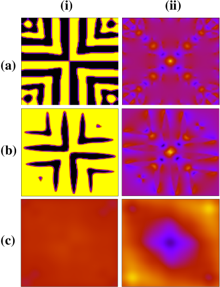
Figure 2: (a)(i) Plot of $e_{3}$ showing the quenched microstructure. The parameters are $\rho=1,a_{3}=0.04,b_{3}=-6,d_{3}=4,c_{3}=4,a_{1}=4,c_{1}=0.04,a_{2}=0.04,c_{p}=0.04,\gamma=20,\xi=0.4,\sigma_{1c}=1$ and $h_{1}=10$. (ii) Corresponding plot of the affine strain $e_{1}^{A}$. (b)(i) The micro- structure and (ii) $e_{1}^{A}$ when the system is placed under an external shear stress. The parameter $\sigma_{3}=0.5$. (c)(i) The order parameter when the system is “heated” by increasing $a_{3}$ from $0.04$ to $4$. The entire system goes into a square phase phase with $e_{3}=0$. (ii) The remnant volumetric strain $e_{1}^{A}$ averages to zero. The color range is from -1 (black) to 0 (brown) to 1 (yellow) for (i)(a),(b)&(c). For (ii)(a),(b)&(c) the corresponding range is from -.1 (black) to .1 (yellow).

III Results

As mentioned before, we look for shape reversibility at the conclusion of the following transformation protocol. Firstly, a finite size solid initially in the shape of a square with a parent (square or $p4mm$) crystal structure (Fig. 1 curve I)is quenched to get a rhombic martensitic product with a $p2$ structure (Fig. 1 curve II). Next, the product phase is deformed (Fig. 1 curve III) with the help of an external shear strain $\sigma_{3}$. Finally, the deformed system is transformed back to the parent square crystal structure (Fig. 1 curve I). All throughout we keep track of the shape using Eqs.(II) and (II). If the system returns to the square shape after heating, we conclude that the shape is reversible, otherwise not. We have performed this transformation protocol for two cases: Case I- when there is only NOP plasticity and no OP plasticity Case II- when plasticity is present in both NOP and OP sector. We give below these results for the two cases, one after the other.

III.1 Case-I

We first consider the case where plasticity exists only in the NOP sector. We need to solve Eqs.(9) and (13) to get the desired quenched microstructure from the parent square phase. Our initial values of $e_{3}(\mathbf{r})$ and $e_{1}^{A}(\mathbf{r})$ are zero everywhere. For the plastic strain $e_{1}^{P}$, we assume $e_{1}^{P}(\mathbf{r},0)=\delta(x-L/2)(y-L/2)$ at $t=0$. When quenched below the transformation temperature, the OP strain $e_{3}$ shows the formation of twins, originating from the center of the simulation box where the initial value of the plastic strain was nonzero [see Fig(2)(a)(i)]. Fig(2)(a)(ii) shows the affine NOP strain $e_{1}^{A}$. The calculated shape of the quenched solid is shown in Fig(3)(a)(i). Although alternating twins are present, the overall shape of the solid continues, on an average, to be a square.

We then load the microstructure using an external shear stress so that only one of the product variants is favored. The system prefers to go to a single variant in order to lower the free energy. We stop the evolution after the system has undergone sufficient deformation. The plots of the OP strain $e_{3}$ and the affine NOP strain $e_{1}^{A}$ is shown in Fig(2)(b). The shape of this deformed system is shown in Fig(3)(b)(i).

Having deformed the system, we transform it back to the parent phase by increasing $a_{3}$ (temprature). The plots of the OP strain $e_{3}$ and the affine NOP strain $e_{1}^{A}$ is shown in Fig(2)(c). The whole system relaxes to zero OP strain. The final shape of the system is plotted in Fig(3)(c)(i). The system goes back to the parent phase, i.e., a square phase, and, at the same time recovers its shape at the end of the complete transformation cycle. The plasticity in the NOP sector does not affect shape recovery because the $e_{1}^{P}$ alternate in sign and average to zero over the entire sample. The shape is determined mainly by the OP strain which is completely reversible.

Figure 3: (a)(i) - (c)(i) The shape of the system corresponding to quenched, loaded and heated microstructure in Fig. (2) and (a)(ii) - (c)(ii) Fig. (4).

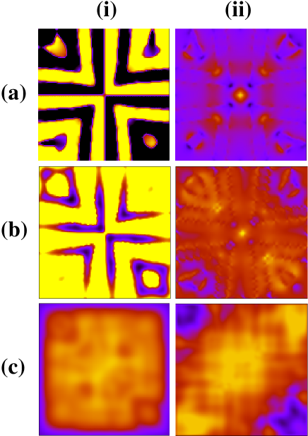
Figure 4: (a)(i) Plot of $e_{3}^{A}$ for the quenched microstructure.(ii) Corresponding plot for $e_{1}^{A}$. (b)(i) Plot for $e_{3}^{A}$ for the deformed microstructure.(ii) Corresponding plot for $e_{1}^{A}$. (b)(i) Plot for $e_{3}^{A}$ after heating the system.(ii) Corresponding plot for $e_{1}^{A}$. $\sigma_{3c}=2$ and $h_{3}=1$. All other parameters are same as that of Fig(2). For (i)(a)-(c), the color range in from -1.5 (black) to 1.5 (yellow) For (ii)(a)-(c), the color range goes from -0.1(black) to 0.1(yellow).

III.2 Case II

We now look into a system undergoing square to rhombic transition including plasticity in the OP sector as well. As before, we start with a solid in the shape of a square and in the $p4mm$ phase with a delta function NOP plasticity at the center of the simulation box and let the system evolve without any external stress to obtain the microstructures. The plots for the affine OP strain $e_{3}^{A}$ and the affine NOP $e_{1}^{P}$ are shown in Fig. 4(a). Note that these, as well as the calculated external shape, shown in Fig. 3. (a)(ii), are not significantly different from those obtained in Case I.

The quenched microstructure, so obtained, is then, as before, deformed with an external shear stress as in the previous case. Unlike Case I, however, the external deformation now has two effects. Firstly, as before, the external stress favors one of the twin variants over the other and therefore alters the microstructure by changing the distribution of the variants. Secondly, the external stress may cause the solid to flow, so that a part of the deformation, would now be plastic. The amount of strain which appears as the plastic strain in the OP sector, of course, depends on the parameters eg $\sigma_{3c}$ - the threshold stress and $h_{3}$ - the rate of plastic strain production. In the present work, we have used a low value of the stress threshold to over-emphasize the plastic contribution for the sake of illustration. In reality, the contribution of the plastic strain may be smaller. The plots of the affine OP strain $e_{3}^{A}$ and the affine NOP $e_{1}^{P}$ are shown in Fig(4)(b). We use the obtained strains to evaluate the displacements at the boundary and hence the shape of the system which is plotted in Fig(3)(b)(ii).

The system is then transformed by increasing $a_{3}$ and the resulting $e_{3}^{A}$ and $e_{1}^{A}$ are plotted in Fig(4)(c). There are remnant (plastic) shear strains in the system even after the solid is fully transformed so that the system fails to go back to the initial square shape as can be seen from the plot of Fig(3)(c)(iii) although the crystal structure is $p4mm$ everywhere as expected. The shape of the solid is now not only determined by the affine OP strain $e_{3}^{A}$ but also, by the plastic part $e_{3}^{P}$ which is not recovered on increasing $a_{3}$. Ultimately this contribution causes shape irreversibility.

IV Summary and conclusion

Using atomistic computer simulations of a model solid, we had shown in Ref.nanomart that group-nonsubgroup transformations are irreversible because plasticity is automatically generated in the OP sector during such transformations in agreement with the conclusions of Bhattacharya et al.kaushik . We showed further that if OP parameter plasticity is suppressed by increasing the yeild stress or in a small system, even group-nonsubgroup transformations may become reversible. In this paper, we complete this line of reasoning by showing explicitly that for shape recovery it is sufficient that all plastic strains be associated exclusively with the NOP sector of the transformation. If, on the other hand, OP plasticity is present, complete shape recovery is impossible. We show this here using an elastoplastic theory where it is possible to control the detailed nature and extent of the plastic strains by varying parameters. If OP plasticity is therefore “artificially” introduced in a group - subgroup ($p4mm\rightleftharpoons p2$) the normally reversible transformation becomes irreversible. Our results may be verified experimentally using shape memory alloys with known and non-trivial yeild criteria such that plasticity in either sector may be controlled independently of each other. We await such systematic studies on the effect of plasticity on shape reversibility.

Before we end, we would like to discuss several possible extensions of this work which we take up one by one as follows.

Stress induced martensite: Within our formalism it is straightforward to consider the effect of plastic deformation on stress induced martensitic transformationspaper0 . Stress- strain hysteresis, which can be routinely measured in such systems may show nontrivial effects due to plasticity at various spatial and temporal scales. The separate effects of NOP and OP plasticity should be explicit in such studies which are planned in the near future.

Scale dependent reversibility: Reversibility of a transformation is, obviously, scale dependent. We have studied here is the question of shape reversibility, namely, reversibility at the largest scale available to the system. In contrast, complete microscopic reversibility would imply that the very positions of atoms be recovered as the transformation is reversed - an impossibility considering the identity of atoms and thermal noise. At intermediate scales, one may ask whether microstructural features are reversible or not below a certain “irreversibility length”. Such calculations are in progress and will be published elsewhere.

Complex dynamics and defect reorganization: The non uniform plastic strain fields created during the transformation are redistributed as the solid is cycled through the transformation protocol many times. It is legitimate to ask whether this distribution has a steady state and what its dynamic properties may be. Defect redistribution and aging during transformation with nontrivial dynamical signatures have been observed in real systemsplanes . We plan to study such questions, as well, within our elastoplastic approach in the future.

V Acknowledgements

Stimulating discussions with A. Saxena, K. Bhattacharya, T. Lookman, R. Ahluwalia, E. Salje and A. E. Jacobs are gratefully acknowledged.

References

- (1) Olson, G. B. Owen, W. (eds) Martensite, (ASM International, Materials Park, OH, 1992), K. Bhattacharya Microstructure of Martensite, (Oxford University Press, Oxford, 2003).
- (2) Otsuka, K. Wayman, C. M. Shape Memory Materials (Cambridge Univ. Press, Cambridge, 1998)
- (3) K. Bhattacharya, S. Conti, G. Zanzotto and J. Zimmer, Nature 428, 55-59, (2004)
- (4) J. Bhattacharya, S. Sengupta and M. Rao, J. Stat. Mech. (2008) P06003.
- (5) J. Bhattacharya, A. Paul, S. Sengupta and M. Rao, J. Phys.: Condens. Matter 20 (2008) 365210.
- (6) D. M. Hatch, T. Lookman, A. Saxena and H. T. Stokes, Phys. Rev. B 64 060104(R) (2001).
- (7) A. Paul, J. Bhattacharya, S. Sengupta and M. Rao, J. Phys.: Condens. Matter 20 (2008) 365211.
- (8) L. D. Landau and E. M. Lifshitz, Theory of Elasticity, (Pergamon Press, Oxford, 1986)
- (9) G. R. Barsch et al., Phys. Rev. Lett.59, 1251 (1987); K. Ø. Rasmussen et al., Phys. Rev. Lett.87, 055704 (2001); T. Lookman et al., Phys. Rev. B67, 024114 (2003), and references therein.
- (10) V. A. Lubarda, Elastoplastic theory, (CRC Press, Boca Raton 2002); J. Lubliner, Plasticity Theory, (Macmillan Publishing, New York, 1990).
- (11) M. Baus and R. Lovett, Phys. Rev. Lett. 65, 1781 1990; 67, 406 1991; Phys. Rev. A 44, 1211 1991.
- (12) F-J Perez-Reché, B. Tadić, L. Mañosa, A. Planes and E. Vives, Phys. Rev. Lett. 93, 195701 (2004); E. Vives, L. Mañosa, R. Ishmael, R. Pérez-Magrané and A. Planes, Phys. Rev. Lett. 72, 1694, (1994).