Correlated Directional Atomic Clouds via Four Heterowave Mixing

Abstract

We investigate the coherence properties of pairs of counter-propagating atomic clouds, produced in superradiant Rayleigh scattering off atomic condensates. It is shown that these clouds exhibit long-range spatial coherence and strong nonclassical density cross-correlations, which make this scheme a promising candidate for the production of highly directional nonclassically correlated atomic pulses.

I Introduction

Atom-atom correlations, and the engineering of “nonclassical” states of atoms that exhibit quantum correlations, are currently attracting intense theoretical and experimental interest in the framework of ultracold quantum gases. In most of these studies, Bose-Einstein condensation plays a central role, since correlated atomic beams can be generated by manipulating appropriately preformed condensates MoleculeBEC ; PuMey00 ; Camp06 ; Aspect-co ; OgrKhe09 ; DeuDru07 ; VogXuKett00 . Directionality of the produced atom pairs, is of vital importance for many potential applications (e.g., subshot noise precision measurements, tests of quantum nonlocality, and presumably quantum information processing) but, as discussed in VarMoo02 , it is difficult to be achieved within existing schemes without seeding (e.g., see VogXuKett00 ).

Superradiant Rayleigh scattering from an elongated atomic condensate InoChiSta99 , has the potential to produce highly directional counter-propagating matter waves, which exhibit correlations as shown in Mey-and-co . Moreover, in contrast to other proposals, the two matter waves have well defined spatial profiles, and one can tune their macroscopic populations. So far, however, the usefulness of the scheme remains debatable, since there has been no theoretical quantitative analysis of the coherence properties of the matter waves, and the type of correlations involved.

Most of these issues are addressed in this article, within a model that treats the scattered photons and the matter waves quantum mechanically. Our model is expected to describe accurately the essential aspects of the process. Moreover, it includes spatial propagation effects, which are crucial for the thorough understanding of condensate superradiance ZobNikPRA , and were not included in Mey-and-co ; You-and-co .

It is shown that the counter-propagating atomic clouds exhibit long-range spatial coherence. Their density cross-correlations are enhanced due to the formation of correlated atom bunches, which are also responsible for violation of the classical Cauchy-Schwarz inequality, relative number squeezing and entanglement. Unlike earlier schemes Camp06 ; Aspect-co ; OgrKhe09 ; DeuDru07 ; VogXuKett00 , we study correlations in the context of mixing two optical– and two matter waves, hence the name “Four Heterowave Mixing”. The present results shed light on the physics of such a mixing process, and they determine the operational regimes for possible applications and future experiments.

II Model

The system involves an elongated condensate of length $L$, oriented along the $z$ axis and consisting of $N$ atoms InoChiSta99 . It is exposed to a linearly polarized pump laser pulse ${\bf E}_{l}({\bf x},t)={\cal E}_{l}(t){\bf e}_{y}[e^{{\rm i}(k_{l}x-\omega_{l}t)}+c.c.]/2$, with $\omega_{l}=ck_{l}$, traveling in the $x$ direction. The laser is assumed to be far off-resonant from any atomic transition, inducing thus Rayleigh scattering.

Due to the coherent nature of the condensate, successive Rayleigh scattering events are strongly correlated, leading to collective superradiant behaviour InoChiSta99 ; Mey-and-co ; You-and-co ; ZobNikPRA . Moreover, as a result of the cigar shape of the condensate, the gain is largest when the scattered photons leave the condensate along its long axis, in the so called endfire modes with momenta ${\bf k}\approx\pm k_{l}{\bf e}_{z}$ and frequency $\omega\approx\omega_{l}$. As a consequence, the recoiling atoms have well-defined momenta and appear in distinct atomic side modes. In the side mode $(n,m)$, atoms possess momentum ${\bf q}\approx\hbar k_{l}(n{\bf e}_{x}+m{\bf e}_{z})$, while the corresponding frequency is approximately given by $\omega_{n,m}\approx(n^{2}+m^{2})\omega_{r}$, where $\omega_{r}=\hbar k_{l}^{2}/2M$ is the recoil frequency, and $M$ the atomic mass. In this notation, the “side mode” $(0,0)$ describes the condensate at rest, while $(1,\pm 1)$ and $(-1,\pm 1)$ are the first-order forward and backward atomic side modes, respectively.

We are here concerned with the early stage of the process, where only first-order atomic side modes become significantly populated. The condensate remains practically undepleted and can be treated as a time-independent classical field $\Phi({\bf x})=\varphi(z)\varphi_{\perp}(x,y)$, where $\varphi(z)$ and $\varphi_{\perp}(x,y)$ are the longitudinal and transverse wave functions. For short times, the coupling between the counter propagating optical end-fire modes can be neglected. Taking advantage of the symmetry of the system with respect to the $x$-axis, we focus on the dynamics of the single endfire mode (taken to be monochromatic with ${\bf k}=+k_{l}{\bf e}_{z}$), and the first-order side modes coupled by it [i.e., $(1,-1)\equiv(+)$ and $(-1,1)\equiv(-)$].

Under the slowly-varying-envelope approximation (SVEA), we decompose the operators for the matter wave and the positive-frequency electric fields as $\hat{\Psi}({\bf x},t)=\Phi({\bf x})+\varphi_{\perp}\sum_{j}\hat{\psi}_{j}(z,t)e^{-{\rm i}[\omega_{j}t-j(k_{l}x-kz)]}$, and $\hat{{\bf E}}^{(+)}({\bf x},t)={\bf E}_{l}^{(+)}({\bf x},t)+\sqrt{\frac{\hbar\omega}{2\varepsilon_{0}}}u_{\perp}\hat{e}(z,t){\bf e}_{y}e^{-{\rm i}(\omega t-kz)}$, with $u_{\perp}(x,y)$ the transverse endfire-mode profile, and $j\in\{+,-\}$. The operators $\hat{\psi}_{j}(z,t)$, $\hat{e}(z,t)$ are annihilation operators for side– and endfire-mode fields with transverse behavior fixed by $\varphi_{\perp}$ and $u_{\perp}$ (see appendix). By construction, these operators obey standard commutation relations with, however, Dirac delta functions having finite width of about $1/k$ (see appendix). Inserting the SVEA expansions into the Maxwell-Schrödinger equations for the coupled matter-wave and electric fields GroHar82 , one can derive equations of motion for the operators $\hat{\psi}_{j}(z,t)$ and $\hat{e}(z,t)$ longpaper . Rescaling to dimensionless time $\tau=2\omega_{r}t$ and length $\xi=k_{l}z$, we obtain

$$\textrm{i}\frac{\partial}{\partial\tau}\hat{\psi}_{+}^{\dagger}(\xi,\tau)=-\kappa\hat{e}(\xi,\tau)\varphi^{*}(\xi),$$ (1a)

$$\textrm{i}\frac{\partial}{\partial\tau}\hat{\psi}_{-}^{\prime}(\xi,\tau)=\kappa\hat{e}(\xi,t)\varphi(\xi)+2\hat{\psi}_{-}^{\prime}(\xi,\tau),$$ (1b)

$$\textrm{i}\left(\frac{\partial}{\partial\tau}+\chi\frac{\partial}{\partial\xi}\right)\hat{e}(\xi,\tau)=\kappa\left[\varphi^{*}(\xi)\hat{\psi}_{-}^{\prime}(\xi,\tau)\right.$$

$$\hskip 113.81102pt\left.+\hat{\psi}_{+}^{\dagger}(\xi,\tau)\varphi(\xi)\right]$$ (1c)

with $\hat{\psi}_{-}^{\prime}=\hat{\psi}_{-}e^{-2{\rm i}\tau}$, $\chi=ck_{l}/(2\omega_{r})$ and $\kappa=g\sqrt{k_{l}L}/(2\omega_{r})$ remark1 . The atom-photon coupling is given by $g=|{\bf d}|^{2}\mathcal{E}_{l}/(2\hbar^{2}\delta)\sqrt{\hbar\omega/(2\varepsilon_{0}L)}\int dxdy\,\varphi_{\perp}^{2}u_{\perp}$, where ${\bf d}$ is the atomic dipole moment, and $\delta$ the detuning of the laser from the nearest atomic transition. By discarding backwards recoiling atomic modes in Eqs. (1), the remaining equations describe conventional superradiance.

Solutions to the system of Eqs. (1) can be expressed as integrals involving the operators evaluated at the boundary of their domain — i.e. at $\xi=0$ and $\tau>0$ or vice versa at $\xi>0$ and $\tau=0$ — by applying Laplace transform techniques. Due to the large value of $\chi$, retardation effects can be neglected, and the solutions for the matter wave operators read longpaper

$$\hat{\psi}_{+}^{\dagger}(\xi,\tau) = \hat{\psi}_{+}^{\dagger}(\xi,0)$$ (2a)

$$+ {\rm i}\kappa\varphi^{*}(\xi)\int_{0}^{\tau}d\tau^{\prime}\hat{e}(0,\tau^{\prime})F_{1,0}(\gamma_{\xi,0},\tau-\tau^{\prime})$$

$$+ \Gamma\varphi^{*}(\xi)\bigg{\{}\int_{0}^{\xi}d\xi^{\prime}\varphi(\xi^{\prime})\hat{\psi}_{+}^{\dagger}(\xi^{\prime},0)F_{2,0}(\gamma_{\xi,\xi^{\prime}},\tau)$$

$$+ \int_{0}^{\xi}d\xi^{\prime}\varphi^{*}(\xi^{\prime})\hat{\psi}_{-}^{\prime}(\xi^{\prime},0)F_{1,1}(\gamma_{\xi,\xi^{\prime}},\tau)\bigg{\}},$$

$$\hat{\psi}_{-}^{\prime}(\xi,\tau) = e^{-{\rm i}2\tau}\hat{\psi}_{-}^{\prime}(\xi,0)$$ (2b)

$$- {\rm i}\kappa\varphi(\xi)\int_{0}^{\tau}d\tau^{\prime}\hat{e}(0,\tau^{\prime})F_{0,1}(\gamma_{\xi,0},\tau-\tau^{\prime})$$

$$- \Gamma\varphi(\xi)\bigg{\{}\int_{0}^{\xi}d\xi^{\prime}\varphi(\xi^{\prime})\hat{\psi}_{+}^{\dagger}(\xi^{\prime},0)F_{1,1}(\gamma_{\xi,\xi^{\prime}},\tau)$$

$$+ \int_{0}^{\xi}d\xi^{\prime}\varphi^{*}(\xi^{\prime})\hat{\psi}_{-}^{\prime}(\xi^{\prime},0)F_{0,2}(\gamma_{\xi,\xi^{\prime}},\tau)\bigg{\}}.$$

We have introduced $\Gamma=\kappa^{2}/\chi$ and the functions $F_{\mu,\nu}(\alpha,\beta)={\mathcal{L}}_{p\to\beta}^{-1}\left\{e^{\alpha/p}e^{-\alpha/(p+2{\mathrm{i}})}p^{-\mu}(p+2{\mathrm{i}})^{-\nu}\right\}$, with ${\mathcal{L}}^{-1}$ denoting the inverse Laplace transform, while $\gamma_{\xi,\xi^{\prime}}=\Gamma\int_{\xi^{\prime}}^{\xi}d\zeta|\varphi(\zeta)|^{2}$. The functions $F_{\mu,\nu}$ can be expressed explicitly as combinations of Bessel functions and integrals thereof (see appendix).

Experimental observations of superradiance from condensates distinguish between the so-called weak- and strong-pulse regimes InoChiSta99 . Typically, the former (WP) regime is characterized by coupling constants $g\sim 10^{5}{\rm s}^{-1}$ and $\Gamma N\simeq 1$, while for the latter (SP) regime $g\sim 10^{6}{\rm s}^{-1}$ and $\Gamma N\gg 1$. Throughout our simulations, we chose $\Gamma N=1$ and $\Gamma N=100$ for the two regimes. The condensate at rest was taken to be Thomas-Fermi distributed, i.e. $\varphi(z)=\sqrt{6(Lz-z^{2})\Theta(z)/L^{3}}$, with $L=130\mu{\mathrm{m}}$ and $\Theta(\cdot)$ the Heaviside step function; containing $N=10^{6}$ ⁸⁷Rb atoms. The incoming laser pulse was chosen to have a rectangular profile and $k_{l}=8.05\times 10^{6}{\mathrm{m}}^{-1}$.

III Coherence and Correlations

The first-order correlation function of the side mode $(j)$ is $G_{jj}^{(1)}(\xi_{1},\xi_{2};\tau)=\langle\hat{\psi}_{j}^{\dagger}(\xi_{1},\tau)\hat{\psi}_{j}(\xi_{2},\tau)\rangle$. It characterizes the coherence properties of the side mode, and quantifies the characteristic coherence length over which phase correlations exist. Using Eqs. (2), the commutation relations for the fields remark3 , and applying the boundary values $\langle\hat{e}^{\dagger}\hat{e}(\xi=0,\tau)\rangle=\langle\hat{\psi}_{j}^{\dagger}\hat{\psi}_{j}(\xi,\tau=0)\rangle=0$ one can easily obtain analytic expressions for $G_{jj}^{(1)}(\xi_{1},\xi_{2};\tau)$ for any time $\tau$. In practice, however, it might not be feasible to resolve the exact atomic positions $\xi_{1}$, and $\xi_{2}$ in the two sidemodes. For direct comparison to possible experiments, we consider the volume averaged degree of coherence, defined as Glauber99

$$\tilde{g}_{jj}^{(1)}(\Delta\xi;\tau)=\frac{\int_{0}^{\Lambda}d\xi_{1}|G_{jj}^{(1)}(\xi_{1},\xi_{1}+\Delta\xi;\tau)|}{\int_{0}^{\Lambda}d\xi_{1}\sqrt{{\cal N}_{jj}(\xi_{1},\Delta\xi;\tau)}},$$

where ${\cal N}_{jj^{\prime}}(\xi_{1},\Delta\xi;\tau)=\langle\hat{n}_{j}(\xi_{1},\tau)\rangle\langle\hat{n}_{j^{\prime}}(\xi_{1}+\Delta\xi,\tau)\rangle$, with $\langle\hat{n}_{j}(\xi,\tau)\rangle=\langle\hat{\psi}_{j}^{\dagger}(\xi,\tau)\hat{\psi}_{j}(\xi,\tau)\rangle$, $\Delta\xi=\xi_{2}-\xi_{1}$ and $\Lambda\equiv k_{l}L$.

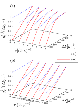
Figure 1: Degree of first-order coherence for the $j$th side-mode at various times, in the WP (a) and SP (b) regimes. The function is symmetric with respect to $\Delta\xi=0$.

As depicted in Fig. 1, $\tilde{g}_{jj}^{(1)}(\Delta\xi;\tau)$ attains its maximum for $\Delta\xi=0$, where $\tilde{g}_{jj}^{(1)}(0;\tau)=1$. Let the coherence length of the side mode $(j)$ be the spatial separation $\lambda_{j}$ for which, $\tilde{g}_{jj}^{(1)}(\lambda_{j};\tau)\approx 1/e$ CohLength . The matter-waves associated with the two side modes can be considered as first-order-coherent for any two points separated by $|\Delta\xi|<\lambda_{j}$. According to Fig. 1, the long-range order of the condensate is transferred to the atoms in the side modes $(\pm)$. More precisely, for relatively short times, the coherence length of the side mode $(+)$ is $\lambda_{1}\approx\Lambda$, while for the side mode $(-)$ it is somewhat smaller $\lambda_{2}\approx 0.6\Lambda$. This is because backward recoiling atoms are created when incoherent light of the endfire mode is scattered by condensed atoms (as opposed to forward recoiling atoms, which involve scattering of coherent laser light), and thus the transfer of coherence is not as efficient as for the side mode $(+)$. In the SP regime, the coherence length of the side mode $(+)$ decreases as time goes on, approaching the one of the backward side mode, which remains practically constant. In the WP regime, however, the corresponding drop is not so prominent, and instead we observe a growth of the spatial coherence for the side mode $(-)$.

Density correlations are described through the second-order correlation functions $G^{(2)}_{jj^{\prime}}(\xi_{1},\xi_{2};\tau)=\langle:\hat{n}_{j}(\xi_{1},\tau)\hat{n}_{j^{\prime}}(\xi_{2},\tau):\rangle$. This quantity reflects the probability of finding an atom of type $(j^{\prime})$ at a position $\xi_{2}$, given that an atom of type $(j)$ has been detected at position $\xi_{1}$. Using Eqs. (2), one can express $G^{(2)}_{jj^{\prime}}(\xi_{1},\xi_{2};\tau)$ in terms of first-order correlation functions. The corresponding volume averaged normalized correlation functions can be defined in analogy to $\tilde{g}_{jj}^{(1)}$ Glauber99 , obtaining

$$\tilde{g}_{jj^{\prime}}^{(2)}(\Delta\xi;\tau) = 1+\frac{\int_{0}^{\Lambda}d\xi_{1}|\rho_{jj^{\prime}}(\xi_{1},\xi_{1}+\Delta\xi;\tau)|^{2}}{\int_{0}^{\Lambda}d\xi_{1}{\cal N}_{jj^{\prime}}(\xi_{1},\Delta\xi;\tau)},$$ (3)

for $\rho_{jj}=G_{jj}^{(1)}(\xi_{1},\xi_{2};\tau)$ and $\rho_{+-}=\langle\hat{\psi}_{+}(\xi_{1},\tau)\hat{\psi}_{-}(\xi_{2},\tau)\rangle$.

In view of Eq. (3), the function $G_{jj}^{(1)}(\xi_{1},\xi_{2};\tau)$ determines to a large extent the density autocorrelation function $\tilde{g}_{jj}^{(2)}(\Delta\xi;\tau)$. The behavior of $\tilde{g}_{jj}^{(2)}(\Delta\xi;\tau)$ throughout the evolution of the system resembles the behavior of the first-order coherence, albeit with somewhat different profiles, not shown here. In contrast to $\tilde{g}_{jj}^{(1)}(\Delta\xi;\tau)$, however, $\tilde{g}_{jj}^{(2)}(0;\tau)\to 2$, as $|\Delta\xi|\to 0$. This is a manifestation of correlations between atomic densities at two different points separated by $|\Delta\xi|\ll\lambda_{j}$. In other words, the recoiling atoms in the side mode $(j)$ tend to appear bunched and thus, detecting an atom in position $\xi_{1}$, significantly increases the probability of detecting another atom close to it. The spatial extent of atom bunches is of the order of $\lambda_{j}$. For $|\Delta\xi|>\lambda_{j}$, $\tilde{g}_{jj}^{(2)}(0;\tau)\to 1$, indicating that atomic densities become uncorrelated for larger separations.

Density cross-correlations between the two side modes, are described through $\tilde{g}_{+-}^{(2)}(\Delta\xi,\tau$), which is plotted in Fig. 2. For any time $\tau$, there is a discontinuity at $\xi_{1}=\xi_{2}$ due to one of the terms in $\rho_{+-}$, which involves $\Theta(\xi_{1}-\xi_{2})$. The physical reason for this discontinuity is the fact that an atom at $\xi_{1}$ in the sidemode ($+$) can be correlated to another atom at $\xi_{2}$ in the sidemode ($-$), only when the latter is created by scattering the endfire photon that was emitted by the former. This process (to be referred to as photon exchange hereafter) is only possible for $\xi_{2}\geq\xi_{1}$ since endfire photons possess momenta $+k{\bf e_{z}}$.

Figure 2: Normalized density cross-correlation function at two different times. (a) WP regime: $\tau=1.025$ $(+)$, $\tau=4.025$ $(\Box)$; (b) SP regime: $\tau=0.03025$ $(+)$, $\tau=0.12075$ $(\Box)$.

The enhanced correlations observed in Fig. 2 for $|\Delta\xi|<\lambda_{+}$, arise through the interplay between atom bunching, exhibited by the side mode $(+)$, and photon exchange. A recoiling atom of type $(-)$, is not correlated only to the atom of type $(+)$ that has emitted the photon, but rather to the entire bunch. Moreover, due to bosonic enhancement, the production of a backward-recoiling atom at a given position, stimulates the creation of additional atoms of the same type nearby. We have thus the production of correlated atomic bunches of type $(+)$ and $(-)$. This is clear in Fig. 2, where the cross-correlation function is always larger than unity, and increases with decreasing $|\Delta\xi|$, attaining its maximum value for $\Delta\xi\to 0^{\pm}$. Thus, measuring an atom in one mode significantly increases the probability of measuring one in the counter-propagating mode. The spatial dependence $g_{+-}^{(2)}(\Delta\xi,\tau)$ at various times, bears analogies to the corresponding behavior of $g_{jj}^{(1)}(\Delta\xi,\tau)$. As a general remark, in the SP regime, we find a much faster decay of $g_{+-}^{(2)}(\Delta\xi,\tau)$ compared to the WP regime.

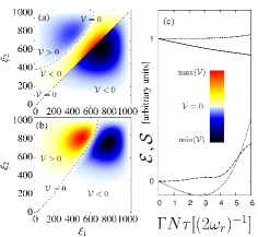
Figure 3: (Color Online) (a,b) Density plots of ${\mathcal{V}}$ at $\Gamma N\tau\simeq 3$. (c) Time evolution of ${\cal S}$ (upper) and ${\cal E}$ (lower). WP regime: (b), dashed and dot-dashed lines; SP regime: (a), solid and dotted lines.

A further, qualitative analysis of correlations can be obtained by means of inequalities. It is known that “classical” fields satisfy the inequality ${\mathcal{V}}(\xi_{1},\xi_{2};\tau)\leq 0$ with ${\mathcal{V}}=[G^{(2)}_{+-}(\xi_{1},\xi_{2};\tau)]^{2}-G^{(2)}_{++}(\xi_{1},\xi_{1};\tau)G^{(2)}_{--}(\xi_{2},\xi_{2};\tau)$, for all times $\tau$ and pairs $(\xi_{1},\xi_{2})$ Glauber99 . A quantum field, however, can violate this inequality if its P-representation attains negative values in a certain region of space and/or time. As depicted in Figs. 3(a,b), in our system, photon exchange may lead to violation of this inequality only for $\xi_{2}\gtrsim\xi_{1}$. Such a violation can be also associated with squeezing or entanglement. The squeezing in the population difference between the two side modes is quantified by, $\mathcal{S}(\tau)=1+\langle{\hat{R}_{+}}\rangle^{-1}\langle:(\Delta\hat{R}_{-})^{2}:\rangle$, where $\Delta\hat{O}=\hat{O}-\langle\hat{O}\rangle$, $\hat{R}_{\pm}(\tau)=\hat{N}_{+}(\tau)\pm\hat{N}_{-}(\tau)$ and $\hat{N}_{j}(\tau)=\int_{0}^{\Lambda}d\xi\hat{n}_{j}(\xi,\tau)$ MoleculeBEC . As depicted in Fig. 3(c), the system exhibits squeezing in the SP regime only where $\mathcal{S}(\tau)<1$. This never happens in the WP regime where $\langle:(\Delta\hat{R}_{-})^{2}:\rangle\approx\int_{0}^{\Lambda}\int_{0}^{\Lambda}d\xi_{1}d\xi_{2}|G_{++}^{(1)}(\xi_{1},\xi_{2};\tau)|^{2}$. A necessary condition for separability of the bipartite system consisting of the modes $(\pm)$ is ${\cal E}\geq 0$, where ${\cal E}(\tau)=\textrm{var}(\hat{A}_{+}+\hat{A}_{-})+\textrm{var}(\hat{B}_{+}-\hat{B}_{-})-C_{+}-C_{-}$, and $C_{j}=|\langle[\hat{A}_{j},\hat{B}_{j}]\rangle|$ Ray-etal . We have checked this inequality for $A_{j}(\tau)=\int_{0}^{\Lambda}d\xi(\psi_{j}+\psi_{j}^{\dagger})$ and $B_{j}(\tau)={\rm i}\int_{0}^{\Lambda}d\xi(\psi_{j}-\psi_{j}^{\dagger})$, which are the quadratures of the side mode $(j)$, with respect to its mean momentum. As depicted in Fig. 3(c), the two side modes are indeed entangled in the SP regime for $0<\Gamma N\tau\lesssim 4.2$. When ${\cal E}\geq 0$, the above criterion does not allow us to infer anything about the entanglement in the system. In view of these results, the SP regime seems to be more interesting for practical purposes than the WP regime.

IV Conclusions

Superradiance from condensates is a promising technique for producing atomic clouds, with well defined momenta, spatial profiles, as well as tunable macroscopic populations. The counter-propagating matter waves typically produced in the strong-pulse regime, exhibit long-range coherence and nonclassical correlations, which can be explored for various applications. Our description does not take multi-modal superradiant emission into account InoChiSta99 ; Mey-and-co , which can be strongly suppressed by reducing the aspect ratio of the condensate InoChiSta99 ; Mey-and-co ; GroHar82 . The main predictions of our model are expected to be valid in more elaborate three-dimensional simulations, which can take into account also the propagation of atoms. In that case, however, the discontinuous gap in $\tilde{g}_{+-}^{(2)}(\Delta\xi;\tau)$ is expected to appear as a sharp but continuous increase. The experimental techniques that have been developed over recent years allow for the direct measurement of correlation functions Aspect-co ; Ritt07 , and should be applicable to the verification of the present theoretical predictions. Finally, some of the present results might also apply to other systems which exhibit similarities to superradiance off condensates such as the collective atomic recoil laser Cola .

The work was supported by the EC RTN EMALI.

Appendix

Appendix A Operator Expansion

Our operators are expanded as

$$\hat{\psi}_{j}(z,t) = \frac{e^{{\mathrm{i}}\omega_{j}t}}{\sqrt{L}}\sum_{p\in\Delta_{0}}e^{ipz}{\hat{c}}_{-jk+p}(t),$$ (4)

$$\hat{e}(z,t) = \frac{e^{i\omega t}}{\sqrt{L}}\sum_{p\in\Delta_{0}}e^{ipz}\hat{a}_{k+p}(t),$$ (5)

where $j\in\{-1,+1\}$, $\omega_{\pm 1}=\frac{k^{2}+k_{l}^{2}}{2M}$ and $\Delta_{0}$ is an interval around zero in momentum space which cannot be chosen larger than $(-k/2,k/2)$ for $\left[\psi_{+}(z,0),\psi_{-}^{\dagger}(z^{\prime},0)\right]=0$ to hold. Therefore the equal field commutator $\left[\psi_{j}(z,0),\psi_{j}^{\dagger}(z^{\prime},0)\right]$ is not a Dirac delta function, but rather a distribution with width of the order $1/k$.

Appendix B Inverse Laplace Transforms

$$F_{1,0}(y,z) = I_{0}\left(2\sqrt{yz}\right)\Theta(z)-\Theta(z)\sqrt{y}\int_{0}^{z}dz^{\prime}\frac{e^{-{\rm i}2z^{\prime}}}{\sqrt{z^{\prime}}}I_{0}\left[2\sqrt{y(z-z^{\prime})}\right]J_{1}\left(2\sqrt{yz^{\prime}}\right)$$ (6a)

$$F_{0,1}(y,z) = e^{-2{\rm i}z}J_{0}\left(2\sqrt{yz}\right)\Theta(z)+\Theta(z)\sqrt{y}\int_{0}^{z}dz^{\prime}\frac{e^{-{\rm i}2z^{\prime}}}{\sqrt{z-z^{\prime}}}I_{1}\left[2\sqrt{y(z-z^{\prime})}\right]J_{0}\left(2\sqrt{yz^{\prime}}\right)$$ (6b)

$$F_{1,1}(y,z) = \Theta(z)\int_{0}^{z}dz^{\prime}e^{-{\rm i}2z^{\prime}}I_{0}\left[2\sqrt{y(z-z^{\prime})}\right]J_{0}\left(2\sqrt{yz^{\prime}}\right)$$ (6c)

$$F_{2,0}(y,z) = \sqrt{\frac{z}{y}}I_{1}(2\sqrt{yz})\Theta(z)-\Theta(z)\int_{0}^{z}{\rm d}z^{\prime}e^{-2{\rm i}z^{\prime}}\sqrt{\frac{z-z^{\prime}}{z^{\prime}}}I_{1}[2\sqrt{y(z-z^{\prime})}]J_{1}[2\sqrt{yz^{\prime}}]$$ (6d)

$$F_{0,2}(y,z) = e^{-2{\rm i}z}\sqrt{\frac{z}{y}}J_{1}(2\sqrt{yz})\Theta(z)+\Theta(z)\int_{0}^{z}{\rm d}z^{\prime}e^{-2{\rm i}z^{\prime}}\sqrt{\frac{z^{\prime}}{z-z^{\prime}}}I_{1}[2\sqrt{y(z-z^{\prime})}]J_{1}[2\sqrt{yz^{\prime}}]$$ (6e)

with $J_{i}$ and $I_{i}$ the $i$th Bessel function of the first kind and the $i$th modified Bessel function respectively.

Appendix C Correlation Functions

$$G^{(1)}_{jj}(\xi_{1},\xi_{2};\tau) = \Gamma M(\xi_{1},\xi_{2})\int_{0}^{\Xi}d\xi^{\prime}|\varphi(\xi^{\prime})|^{2}F_{1,1}(\gamma_{\xi_{2},\xi^{\prime}},\tau)F_{1,1}^{*}(\gamma_{\xi_{1},\xi^{\prime}},\tau),$$

$$+\delta_{j,+}M(\xi_{1},\xi_{2})\int_{0}^{\tau}d\tau^{\prime}F_{1,0}(\gamma_{\xi_{1},0},\tau-\tau^{\prime})F_{1,0}^{*}(\gamma_{\xi_{2},0},\tau-\tau^{\prime}),$$

where $M(\xi_{1},\xi_{2})=\Gamma\varphi(\xi_{1})\varphi(\xi_{2})$, $\delta_{j,j^{\prime}}$ is Kronecker’s delta, and $\Xi={\min(\xi_{1},\xi_{2})}$.

$$G^{(2)}_{jj^{\prime}}(\xi_{1},\xi_{2};\tau) = \langle\hat{n}_{j}(\xi_{1},\tau)\rangle\langle\hat{n}_{j^{\prime}}(\xi_{2},\tau)\rangle+|\sigma_{jj^{\prime}}(\xi_{1},\xi_{2};\tau)|^{2},$$

where

$$\sigma_{jj}(\xi_{1},\xi_{2};\tau)=G^{(1)}_{jj}(\xi_{1},\xi_{2};\tau),$$ (8b)

and

$$\sigma_{+-}(\xi_{1},\xi_{2};\tau) \equiv \langle\hat{\psi}_{+}(\xi_{1},\tau)\hat{\psi}_{-}(\xi_{2},\tau)\rangle$$

$$= -M(\xi_{1},\xi_{2})F_{1,1}(\gamma_{\xi_{2},\xi_{1}},\tau)\Theta(\xi_{2}-\xi_{1})$$

$$-\Gamma M(\xi_{1},\xi_{2})\int_{0}^{\Xi}d\xi^{\prime}|\varphi(\xi^{\prime})|^{2}F_{1,1}(\gamma_{\xi_{2},\xi^{\prime}},\tau)F_{2,0}^{*}(\gamma_{\xi_{1},\xi^{\prime}},\tau),$$

References

- (1) C. M. Savage and K. V. Kheruntsyan, Phys. Rev. Lett. 99, 220404 (2007); M. Greiner et al., ibid. 94, 110401 (2005); M. Ögren and K. V. Kheruntsyan, Phys. Rev. A 78 011602(R) (2008).
- (2) H. Pu and P. Meystre, Phys. Rev. Lett. 85, 3987 (2000); L.-M. Duan et al., ibid. 85 3991 (2000); K. M. Hilligsøe and K. Mølmer, Phys. Rev. A 71 041602(R) (2005).
- (3) G. K. Campbell et al., Phys. Rev. Lett. 96, 020406 (2006).
- (4) A. Perrin et al., Phys. Rev. Lett 99, 150405 (2007).
- (5) M. Ögren and K. V. Kheruntsyan, Phys. Rev. A 79, 021606(R) (2009).
- (6) P. Deuar and P. D. Drummond, Phys. Rev. Lett. 98, 120402 (2007).
- (7) J. M. Vogel, K. Xu and W. Ketterle, Phys. Rev. Lett. 89, 020401 (2002).
- (8) A. Vardi and M. G. Moore, Phys. Rev Lett. 89, 090403 (2002).
- (9) S. Inouye et al, Science 285, 571 (1999); D. Schneble et al., Science 300, 475 (2003).
- (10) M. G. Moore and P. Meystre, Phys. Rev. Lett. 83, 5202 (1999); H. Pu, W. Zhang, and P. Meystre, Phys. Rev. Lett. 91, 150407 (2003).
- (11) O. Zobay and G. M. Nikolopoulos, Phys. Rev. A 72, 041604(R) (2005); 73, 013620 (2006).
- (12) M. E. Tasgin et al., Phys. Rev. A 79, 053603 (2009).
- (13) M. Gross and S. Haroche, Phys. Rep. 93, 301 (1982); W. Zhang and D. F. Walls, Phys. Rev. A 49, 3799 (1994); F. Haake et al., Phys. Rev. A 20, 2047 (1979).
- (14) L. F, Buchmann et al., in preparation.
- (15) We neglect the external trapping potential and the atomic interactions, since they do not play a significant role on the time scales of the process under consideration.
- (16) The finite-width delta functions can be approximated by completely localized ones as they are integrated over slowly varying functions.
- (17) P. Meystre, Atom Optics (Springer-Verlag, New York, 2001); M. Naraschewski and R. J. Glauber, Phys. Rev. A 59, 4595 (1999).
- (18) F. Gerbier et. al., e-print arXiv:cond-mat/0210206.
- (19) M. G. Raymer et. al., Phys. Rev. A 67, 052104 (2003); A. J. Ferris et al.. ibid. 79, 043634 (2009).
- (20) S. Ritter at al., Phys. Rev. Lett. 98, 090402 (2007).
- (21) M. M. Cola, M. G. A. Paris and N. Piovella, Phys. Rev. A 70, 043809