Quantum anomalies and linear response theory

Abstract

The analysis of diffusive energy spreading in quantized chaotic driven systems, leads to a universal paradigm for the emergence of a quantum anomaly. In the classical approximation a driven chaotic system exhibits stochastic-like diffusion in energy space with a coefficient $D$ that is proportional to the intensity $\varepsilon^{2}$ of the driving. In the corresponding quantized problem the coherent transitions are characterized by a generalized Wigner time $t_{\varepsilon}$, and a self-generated (intrinsic) dephasing process leads to non-linear dependence of $D$ on $\varepsilon^{2}$.

A major theme in mechanics concerns the response of a system to a driving source $f(t)$, given that the interaction term is $\mathcal{H}_{\mbox{\tiny int}}=f(t)V$. This leads to the well known framework of linear response theory (LRT) with its celebrated fluctuation-dissipation relation. Below we assume a stationary driving source which is characterized by a power spectrum $\tilde{S}(\omega)=\mbox{FT}[\langle f(t)f(0)\rangle]$, where FT stands for Fourier transform. In the absence of driving the stationary fluctuations of the system are characterized by the spectral function $\tilde{C}(\omega)=\mbox{FT}[\langle V(t)V(0)\rangle]$. In the presence of driving the main three effects are: the decay of the initial preparation; the spreading and eventually the diffusion in energy space; and the associated heating.

1 LRT and Kubo

Strict LRT behavior means that the diffusion in energy space [1] and the related absorption coefficient [2, 3, 4] are linear functional of the spectral function $\tilde{S}(\omega)$. Specifically, the Kubo formula for the diffusion coefficient in energy space is

$$D\ \ =\ \ \frac{1}{2}\int_{-\infty}^{\infty}\omega^{2}d\omega\ \tilde{C}(\omega)\tilde{S}(\omega)$$ (1)

It follows that the diffusion is proportional to the intensity of the driving $\varepsilon^{2}$ as defined below. We are going to consider on equal footing driving by a quasi-constant perturbation $f(t)\,{\sim}\mbox{const}$, and quasi-linear DC driving with $\dot{f}(t)\,{\sim}\mbox{const}$. The notation “${\sim}\mbox{const}$” means that it is constant over large time intervals of duration $t_{\varphi}$, with some characteristic RMS value that we call $\varepsilon$. Accordingly the associated spectral functions is

$$\tilde{S}(\omega)\ \ =\ \ \varepsilon^{2}\omega^{-\sigma}\delta_{\gamma}(\omega)$$ (2)

where $\delta_{\gamma}(\omega)=(\gamma/\pi)/(\omega^{2}+\gamma^{2})$ with $\gamma=1/t_{\varphi}$, while the spectral exponent is $\sigma{=}0$ for quasi-constant perturbation, and $\sigma{=}2$ for quasi linear DC driving.

2 Paradigms

We are looking for circumstances where the Kubo formula is not applicable. This means that either $D$ is still proportional to the strength of the driving but with an anomalous coefficient, or more generally $D$ might depend in a non-linear way on the strength of the driving. Paradigms for non-LRT response with which we are familiar are:  (i) Classical non-LRT route that follows from the Kolmogorov-Arnold-Moser scenario as in the driven (kicked) rotator problem [5];  (ii) Quantum semi-LRT due to sparsity and textures that characterize the perturbation matrix [6];  (iii) Quantum corrections due to dynamical localization effect [7, 8].  (iv) Quantum absorption due to Landau-Zener transitions between neighboring energy levels [2];  (v) Quantum non-perturbative anomalies that are associated with having a finite spectral bandwidth [9].

3 Scope and main observation

One should notice that all the mentioned non-LRT paradigms above become irrelevant if we consider the continuum limit of a universal quantized chaotic system. By definition “continuum” means that the Heisenberg time (see definition later) can be taken as infinite, while “universality” means that the correlation time (see definition later) can be taken as zero. It should be clear that our considerations apply to strictly chaotic systems that do not have mixed phase-space dynamics. In the present work we show that even with all these assumptions and exclusions there is still room for a novel manifestation of quantum mechanical anomalies in the response to external driving. A central role is played by the generalized Wigner time $t_{\varepsilon}$ which characterizes a coherent spreading process in energy space, and by what we call intrinsic dephasing time $t_{\varphi}^{\mbox{\tiny(eff)}}$.

Beyond any technical details it is important to realize that for a universal chaotic system, as assumed in Random Matrix Theory (RMT) studies, the Kubo formula of LRT can be deduced merely via dimensional analysis. The non-Ohmic generalization of this statement [Eq.(10)], as established in this communication, implies a universal quantum anomaly in the response characteristics of non-Ohmic systems. This prediction has potential applications e.g. with regard to the rate of heating of cold atoms in vibrating traps.

4 Modeling

In a system that is described by a time dependent Hamiltonian $\mathcal{H}[R]$ with $R=R_{0}{+}f(t)$ the transitions between the adiabatic energy levels $E_{n}$ are induced by the perturbation matrix $V_{nm}=(d\mathcal{H}/dR)_{nm}$. The spectral function that characterizes the fluctuations of $V$ in the absence of driving is

$$\tilde{C}(\omega)=\sum_{n}|V_{n,n_{0}}|^{2}2\pi\delta\left(\omega-\frac{E_{n}{-}E_{n_{0}}}{\hbar}\right)$$ (3)

with implicit average over $n_{0}$ as determined by the energy window of interest. We assume below that

$$\tilde{C}(\omega)=2\pi|\omega|^{s_{0}-1}\ \ \ \ \ \ \ \ \ \mbox{for $\omega_{0}<|\omega|<\omega_{\mbox{\tiny cl}}$}$$ (4)

and distinguish between the Ohmic ($s_{0}{=}1$), subOhmic ($0{<}s_{0}{<}1$), and superOhmic ($1{<}s_{0}{<}2$) cases. Without loss of generality, by appropriate rescaling of $f(t)$, we set the prefactor in Eq.(4) as $2\pi$. The infrared cutoff ${\omega_{0}=(\hbar\varrho)^{-1}}$ is the mean level spacing, as determined by the density of states. The ultraviolet cutoff $\omega_{\mbox{\tiny cl}}$ is determined by the classical dynamics and is known as the bandwidth or as the ballistic version of the Thouless energy. The associated time scales are the Heisenberg time $t_{\mbox{\tiny H}}=2\pi\hbar\varrho$ and the classical correlation time $t_{\mbox{\tiny cl}}=2\pi/\omega_{\mbox{\tiny cl}}$. In a later paragraph we define the generalized Wigner time $t_{\varepsilon}$ that depends on the strength of the driving. This time scale characterizes the coherent spreading process. We assume below mesoscopic circumstances for which

$$t_{\mbox{\tiny cl}}\ \ll\ (t_{\varepsilon},t_{\varphi})\ \ll\ t_{\mbox{\tiny H}}\ \ \ \ \ \ \ \ \mbox{[mesoscopics]}$$ (5)

where $t_{\varphi}$ is the correlation time of the driving source as define with relation to Eq.(2). Our interest is in results that remain well defined for ${t_{\mbox{\tiny cl}}\rightarrow 0}$ (universal limit) and ${t_{\mbox{\tiny H}}\rightarrow\infty}$ (continuum limit). The existence of a universal limit is the underlying postulate in RMT modeling. We distinguish in the analysis between weak (${t_{\varepsilon}>t_{\varphi}}$) and strong (${t_{\varepsilon}<t_{\varphi}}$) driving.

5 DC driving

The common interest is in Ohmic systems (${s_{0}=1}$) with quasi-linear DC driving (${\sigma=2}$), for which Kubo formula gives $D=\pi\varepsilon^{2}$. This result is not sensitive to $t_{\varphi}$, and is independent of the infrared and ultraviolet cutoffs. Our purpose is to generalize this result for the case of non-Ohmic fluctuations. We shall see that this requires to go beyond LRT.

The key observation is that the problem of quasi-linear DC driving reduces, with some reservations, to the analysis of quasi-constant perturbation. This is done by transforming the Hamiltonian into the adiabatic basis where it takes the form

$$\tilde{\mathcal{H}}=\mbox{diag}\{E_{n}\}+\dot{f}\left\{i\frac{\hbar V_{nm}}{E_{n}-E_{m}}\right\}$$ (6)

If we ignore the implicit time dependence of the adiabatic energies and matrix elements, then this Hamiltonian is the same as that of quasi-constant perturbation but with effective exponent ${s=s_{0}-2}$. In particular quasi-linear driving of an Ohmic system corresponds to ${s=-1}$.

At this point one wonders what is the effect of the residual implicit time dependence of the Hamiltonian Eq.(6). Obviously we should not be too worried about the wiggles of the levels, because they take place on a very small energy scale and would be of relevance only if we were considering times of the order of the Heisenberg time. On the other hand, the variation of the matrix elements cannot be ignored, and we shall come back to this issue later.

6 The generalized Wigner time

Universality (irrelevance of $\omega_{\mbox{\tiny cl}}$) is a common built-in assumption in numerous “quantum chaos” studies that utilize the standard random matrix ensembles. Furthermore a quasi-continuum assumption (irrelevance of $\omega_{0}$) is implicit in the standard derivations of LRT. If we believe that in the continuum limit ($\omega_{0}\rightarrow 0$) there exists a universal limit ($\omega_{\mbox{\tiny cl}}\rightarrow\infty$) that leads to a generalized response theory, then disregarding $t_{\varphi}$ the only relevant time scale that might emerge in the dynamics is implied by dimensional analysis:

$$t_{\varepsilon}\ \ =({\hbar}/{\epsilon})^{2/(2{-}s)}$$ (7)

One immediately realizes that it is the generalized Wigner time of Ref.[10]. For a quasi-constant perturbation of Ohmic system it is literally the Wigner time

$$t_{\varepsilon}=(\hbar/\Gamma_{\mbox{\tiny E}}),\ \ \ \ \ \ \ \ \mbox{for ${s=1}$}$$ (8)

where ${\Gamma_{\mbox{\tiny E}}=(2\pi/\hbar)\epsilon^{2}}$ is the Fermi-golden-rule rate of transitions. For a quasi-linear driving of Ohmic system it is the breaktime scale that has been introduced in Ref.[4],

$$t_{\varepsilon}=(\hbar^{2}/D)^{1/3},\ \ \ \ \ \ \ \ \mbox{for ${s=-1}$}$$ (9)

where $D=\pi\varepsilon^{2}$ in derived from the Kubo formula.

More generally, in the non-Ohmic case, we can associate with the generalized Wigner time an energy scale $\hbar/t_{\varepsilon}$ and a diffusion coefficient

$$D_{\varepsilon}\ =\ \frac{\hbar^{2}}{t_{\varepsilon}^{3}}\ =\ \hbar^{-2\frac{s{+}1}{2{-}s}}\ \varepsilon^{\frac{6}{2{-}s}},\ \ \ \ \ \ \ \ \mbox{[${s=s_{0}{-}\sigma}$]}$$ (10)

At this point one should wonder whether this expression might emerge from the analysis of the spreading process in some universal limit. Note that it is only in the Ohmic (Kubo) case that $D_{\varepsilon}$ becomes $\hbar$ independent.

7 Coherent spreading

If the perturbation matrix in Eq.(6), call it $W_{nm}$, were strictly time independent, then the induced wavepacket dynamics would lead to a steady state, with a saturation profile that reflects the local density of states. Specifically, let us assume that the system is prepared in the unperturbed state $n$ for which the unperturbed energy $E_{n}$ is well defined, then in the perturbed basis it has the energy distribution

$$P_{\infty}(E)=\sum_{\nu}|\langle\nu|n\rangle|^{2}\delta(E{-}E_{\nu})$$ (11)

We have argued in Ref.[10], following previous studies, that this energy distribution has a semicircle-like core that extends within $|E{-}E_{n}|<\hbar/t_{\varepsilon}$, coexisting with outer perturbative tails that are determined by the first order expression $|W_{nm}|^{2}/(E_{n}{-}E_{m})^{2}$ for the overlaps. The associated variance is $\Delta E(\infty)^{2}=\omega_{\mbox{\tiny cl}}^{s}\varepsilon^{2}$ for $s>0$, and $\Delta E(\infty)^{2}=(\hbar/t_{\varepsilon})^{2}$ for $s<0$.

In the time dependent analysis the steady state profile of $P_{t}(E)$ is achieved only after $t_{\varepsilon}$, but the crossover is not necessarily observed in the spreading $\Delta E(t)$, which is a second moment calculation. Specifically we get

$$\Delta E(t)= \varepsilon\ \omega_{\mbox{\tiny cl}}^{s/2}\ \ \ \ \ \ s{>}0 t{>}t_{\mbox{\tiny cl}}$$ for [],[] (12)

$$\Delta E(t)= \varepsilon\ t^{|s|/2}\ \ \ \ \ \ s{<}0 t_{\mbox{\tiny cl}}{<}t{<}t_{\varepsilon}$$ for [],[] (13)

$$\Delta E(t)= \hbar/t_{\varepsilon}\ \ \ \ \ \ s{<}0 t{>}t_{\varepsilon}$$ for [],[] (14)

For ${s>0}$ the spreading saturates as soon as $t>t_{\mbox{\tiny cl}}$, and to detect the crossover at $t_{\varepsilon}$ one should look on the survival probability or on percentiles of the distributions as described in Ref.[10]. But for ${s<0}$ the second moment of the evolving distribution exhibits the crossover to saturation at $t_{\varepsilon}$, and not at $t_{\mbox{\tiny cl}}$. This can be deduced using the following simple reasoning. First order perturbation theory implies that the tail grows like $|W_{nm}t|^{2}$ within the shrinking interval ${\hbar\gamma(t)<|E-E_{n}|<\hbar/t}$. In the outer ${|E{-}E_{n}|>\hbar/t}$ region the tail is saturated due to recurrences. The lower cutoff $\gamma(t)$ is determined by a self-consistency condition, saying that the integral over the 1st order tail of $P_{t}(E)$ from $\gamma(t)$ to infinity should be $\mathcal{O}(1)$. This leads to the estimate ${\gamma(t)=\left[t^{|s|}+(\varepsilon t/\hbar)^{-2}\right]^{-1/|s|}}$. Steady state is achieved at $t_{\varepsilon}$ when ${\gamma(t)\sim 1/t}$. Up to this time the second moment of the evolving distribution is dominated by the growing piece of the tail leading to Eq.(13). This is a diffusive-like growth (${\Delta E(t)\propto t^{1/2}}$) in the case of a quasi-linear DC driving.

8 Diffusion

The dephasing time $t_{\varphi}$ indicates the crossover from coherent to stochastic spreading behaviour. The central limit theorem implies that the long time spreading is diffusive with coefficient

$$D=\frac{\Delta E(t_{\varphi})^{2}}{2t_{\varphi}}$$ (15)

where $\Delta E(t)$ is the time dependent coherent spreading that we have discussed in the previous paragraph. This result is classical in nature (no $\hbar$) and it is easily checked that it agrees with the Kubo formula Eq.(1) provided we use Eq.(12) or Eq.(13), leading to

$$D\ \ = \varepsilon^{2}\ \omega_{\mbox{\tiny cl}}^{s}\ t_{\varphi}^{-1}\ \ \ \ \ \ \ \ \ s{>}0$$ for [] (16)

$$D\ \ = \varepsilon^{2}\ t_{\varphi}^{|s|{-}1}\ \ \ \ \ \ \ \ \ s{<}0 t_{\varphi}{<}t_{\varepsilon}$$ for [],[] (17)

Both results are $\propto\varepsilon^{2}$. In particular Eq.(16) applies to quasi-constant perturbation and is merely the well known hopping estimate for the noise-induced diffusion is system with ‘localization’.

Consider a general system with quasi-linear DC driving, such that ${s<0}$. If the driving is weak (${t_{\varphi}<t_{\varepsilon}}$) it is justified to substitute Eq.(13) in Eq.(15), thus getting the LRT result Eq.(17). In particular we note that in the standard case of DC-driven Ohmic system (${s=-1}$) we get a $t_{\varphi}$ independent result. Otherwise the result is $t_{\varphi}$ dependent. For ${|s|\neq 1}$ one observes that in the limit ${t_{\varphi}\rightarrow\infty}$ the LRT result is either zero or infinity. This suggests that in such circumstances a realistic theory should lead to an $\hbar$ dependent result.

9 Beyond LRT

So far the elaborated spreading picture that we have introduced gave for $D$ the same result as Kubo. So now we would like to see whether there are circumstances where this picture leads to novel physics beyond LRT. Considering ${s<0}$ and strong driving ${t_{\varepsilon}<t_{\varphi}}$, it seems that one should substitute Eq.(14) in Eq.(15), leading to a sub-linear dependence on the strength of the driving:

$$D\ \ =\ \ \hbar^{\frac{2|s|}{2{+}|s|}}\varepsilon^{\frac{4}{2{+}|s|}}\ t_{\varphi}^{-1},\ \ \ \ \ \ \ \ \ [s{<}0],[t_{\varphi}{>}t_{\varepsilon}]$$ (18)

However, one should be critical with regard to this result. The saturation of the coherent spreading process assumes a time-independent perturbation in Eq.(6). This would be the case if ${\sigma=0}$ but not if ${\sigma=2}$.

10 Intrinsic dephasing hypothesis

Considering the general problem of having a driving source with arbitrary spectral exponent $\sigma$, one realizes that as far as the integrand of the Kubo formula Eq.(1) is concerned the effective spectral exponent is ${s=s_{0}-\sigma}$. If a breakdown of this spectral equivalence rule is observed, it constitutes a demonstration of a quantum anomaly. Indeed in the numerical experiment of Fig. 1, we contrast the dynamics which is generated by a time-dependent ($\sigma{=}-2$) perturbation, with that of a frozen ($\sigma{=}0$) perturbation that has the same $s$. We find that only the latter shows the coherent saturation of Eq.(14).

Consequently we would like to conjecture that the implicit time-independence of the perturbation in Eq.(6) leads to an intrinsic dephasing time $t_{\varphi}^{\mbox{\tiny eff}}$ which is finite in the limit ${t_{\varphi}\rightarrow\infty}$. We have in our problem only one time scale, the generalized Wigner time, and therefore the natural speculation would be $t_{\varphi}^{\mbox{\tiny eff}}\sim t_{\varepsilon}$. If this speculation is true, then the replacement ${t_{\varphi}\mapsto t_{\varphi}^{\mbox{\tiny eff}}}$ in Eq.(18) leads to the universal result Eq.(10). For the standard Ohmic case this implies that diffusive spreading persists beyond $t_{\varepsilon}$, and that LRT-like result ${\propto\varepsilon^{2}}$ still holds. For the non-Ohmics case this implies that the sub-diffusive or super-diffusive coherent spreading turns into normal diffusion with non-linear dependence on ${\varepsilon^{2}}$. Both expectations are supported by the numerical experiment of Fig.1 that we further discuss and analyze below.

11 RMT numerics

In order to have a model that captures and tests the question of spectral equivalence it is convenient to use not the standard Wigner model, but rather its parametric invariant variation:

$$\mathcal{H}_{ij}(t)\ =\ \mathcal{E}_{i}\delta_{ij}+\cos[f(t)]\ V^{(1)}_{ij}+\sin[f(t)]\ V^{(2)}_{ij}$$ (19)

where $V^{(1)}_{ij}$ and $V^{(2)}_{ij}$ are two independent realizations of a banded matrix, that has a bandprofile $\lambda|\omega|^{s_{\lambda}-1}$, in the sense of Eq.(3), but with ${n\mapsto i}$. The energies $E_{n}(t)$ are obtained via diagonalization of $\mathcal{H}(t)$ and the perturbation matrix $V_{nm}(t)$ should be written in the same basis. The bandprofile of $V_{nm}$ is related to that of $V_{ij}$ as discussed in [11]. We have set $\varrho{=}1$ and $\lambda{=}1$ and verified that ${s_{0}\approx s_{\lambda}}$. We consider DC driving $\dot{f}=\mbox{const}$, and accordingly ${\varepsilon^{2}=\lambda\dot{f}^{2}}$.

In the time dependent adiabatic basis the perturbation matrix in the transformed Hamiltonian Eq.(6) is $W_{nm}(t)=i\dot{f}V_{nm}/(E_{n}{-}E_{m})$, whose bandprofile is characterized by $s=s_{0}{-}2$. This matrix changes with time but it preserves its statistical properties. The question is whether its implicit time dependence generates an effective dephasing process.

The numerical experiment is simple. On the one hand we make simulations with the time dependent Hamiltonian $\mathcal{H}$. On the other hand we use a frozen version of Eq.(6) which we write in the $ij$ basis as

$$\mathcal{H}_{ij}(\mbox{\small frozen})\ =\ \mathcal{E}_{i}\delta_{ij}+U_{ij}+\dot{f}\ W_{ij}(0)$$ (20)

The initial state is assumed to be localized at ${i=0}$, and an ensemble average over realizations is taken. Comparing the simulations (Fig.1) we deduce that there is intrinsic dephasing due to the implicit time dependence of the driving in Eq.(6).

In order to figure out what is the intrinsic dephasing time we plot in Fig.2 the scaled diffusion $D/D_{\varepsilon}$ versus the strength of the driving. The Ohmic case as conjectured is ‘boring’. In contrast to that the sub-Ohmic and the super-Ohmic case exhibit departure from the universal expectation for large and small $\varepsilon$ respectively, indicating that the effective dephasing time becomes shorter than $t_{\varepsilon}$. We associate this systematic deviation with the infrared and ultraviolet cutoffs respectively: otherwise dimensional analysis implies that such deviation cannot emerge. We explain this sensitivity as follows: The value of $D$ is most sensitive to $t_{\varphi}$ in the slow diffusion stage. In the sub (super) Ohmic case the slow diffusion stage is for long (short) times, and accordingly the sensitivity is to the lower (upper) cutoff, in-spite of the fact that the spreading is dominated by the high (low) frequency transitions.

12 Conclusions

LRT gives a finite classical-like result for the response of a low frequency driven Ohmic system. But in the case of a sub-Ohmic or super-Ohmic system, classical LRT predicts in the same limit either zero or infinite response. This is the notch where quantum-mechanics becomes most relevant, leading to an anomalous non-linear response.

The analysis highlights the role which is played by the generalized Wigner time of [10], which is the only relevant time scale in the universal continuum limit, and leads to a single-parameter expression Eq.(10) for the diffusion in energy space.

The results might have a direct application concerning the heating rate of cold atoms in vibrating traps [12], where the experimentalist has control over both the shape (hence $\tilde{C}(\omega)$) and the power spectrum ($\tilde{S}(\omega)$) of the driving. In particular we note that if cold atoms are “shaken” without deforming the shape of the billiard, the spectral function that describes the fluctuations becomes sub-Ohmic [13].

References

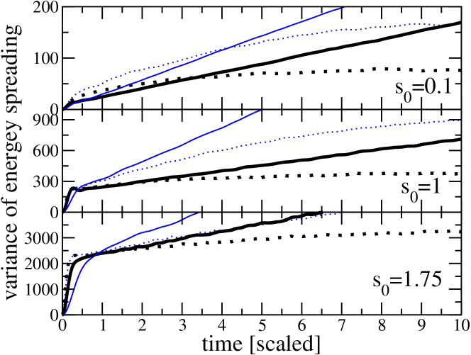
Figure 1: (color online) Variance of energy spreading versus time for three different $s_{0}$-values, and two different driving rates $\dot{f}{=}5$ (thick black lines) and $\dot{f}{=}12$ (thin blue lines). The time-axis is rescaled according to the Wigner time $t_{\epsilon}$ given by Eq.(7). Solid lines correspond to the simulations based on the Hamiltonian of Eq.(19), while the dotted are for its frozen version Eq.(20).

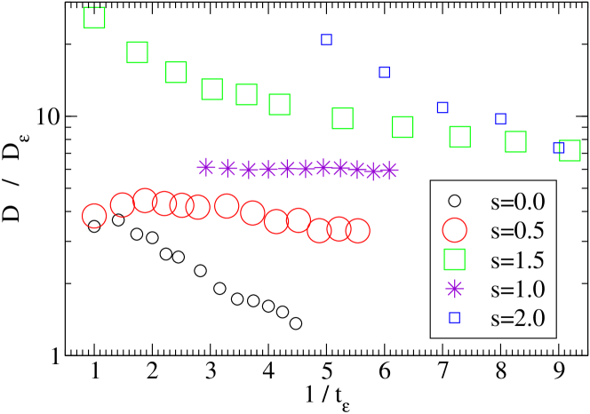
Figure 2: (color online) Dependence of diffusion on the rate of the driving for various values of $s_{0}$. The axes are $X=\varepsilon^{2/(2{-}s)}$ and $Y=D/\varepsilon^{6/(2{-}s)}$, where $s=s_{0}{-}2$. Note that ${\omega_{0}<X<\omega_{\mbox{\tiny cl}}}$ where the level spacing is ${\omega_{0}=1}$ and the bandwidth is ${\omega_{\mbox{\tiny cl}}=50}$. The deviation of $D$ from universlity is due to the finite infrared or ultraviolet cutoffs: We see that in the superOhmic case (${s_{0}>1}$) the diffusion $D$ becomes $\omega_{0}$ independent for large $\varepsilon$, while in the subOhmic case (${s_{0}<1}$) it becomes $\omega_{\mbox{\tiny cl}}$ independent for small $\varepsilon$.

References

- [1] E. Ott, Phys. Rev. Lett. 42, 1628 (1979). R. Brown, E. Ott and C. Grebogi, Phys. Rev. Lett, bf 59, 1173 (1987); J. Stat. Phys. 49, 511 (1987).
- [2] M. Wilkinson, J. Phys. A 21, 4021 (1988); J. Phys. A 20, 2415 (1987).
- [3] C. Jarzynski, Phys. Rev. E 48, 4340 (1993); Phys. Rev. Lett. 74, 2937 (1995).
- [4] D. Cohen, Annals of Physics 283, 175 (2000).
- [5] A.J. Lichtenberg and M.A. Lieberman, Regular and Stochastic Motion, (Springer, Berlin, 1983).
- [6] D. Cohen, T. Kottos and H. Schanz, J. Phys. A 39, 11755 (2006). M. Wilkinson, B. Mehlig and D. Cohen, Europhys. Lett. 75, 709 (2006). See also: A. Stotland, T. Kottos and D. Cohen, Phys. Rev. B 81, 115464 (2010).
- [7] For review and references see lecture notes by M. Raizen, in ”Quantum Chaos”, Proceedings of the International School of Physics ”Enrico Fermi”, Course CXLIII, Ed. G. Casati, I. Guarneri and U. Smilansky (IOS Press, Amsterdam 2000).
- [8] D.M. Basko, M.A. Skvortsov and V.E. Kravtsov, Phys. Rev. Lett. 90, 096801 (2003).
- [9] D. Cohen, Phys. Rev. Lett. 82, 4951 (1999). D. Cohen and T. Kottos, Phys. Rev. Lett. 85, 4839 (2000).
- [10] J. Aisenberg, I. Sela, T. Kottos, D. Cohen and A. Elgart, J. Phys. A 43, 095301 (2010); I. Sela et al, Phys. Rev. E 81, 036219 (2010).
- [11] J.A. Mendez-Bermudez, T. Kottos and D. Cohen, Phys. Rev. E 73, 036204 (2006).
- [12] M. Andersen, A. Kaplan, T. Grunzweig, N. Davidson, Phys. Rev. Lett. 97, 104102 (2006). A. Stotland, D. Cohen, N. Davidson, Europhys. Lett. 86, 10004 (2008).
- [13] A. Barnett, D. Cohen and E.J. Heller, Phys. Rev. Lett. 85, 1412 (2000); J. Phys. A 34, 413 (2001).