Identifying the starting point of a spreading process in complex networks

Abstract

When dealing with the dissemination of epidemics, one important question that can be asked is the location where the contamination began. In this paper, we analyze three spreading schemes and propose and validate an effective methodology for the identification of the source nodes. The method is based on the calculation of the centrality of the nodes on the sampled network, expressed here by degree, betweenness, closeness and eigenvector centrality. We show that the source node tends to have the highest measurement values. The potential of the methodology is illustrated with respect to three theoretical complex network models as well as a real-world network, the email network of the University Rovira i Virgili.

I introduction

In complex network research, it is usual to study dynamics that have a source, that is, the process taking place in the network originates from a well-defined set of nodes, which can be sparse, appearing in many places of the system, or clustered. There are many examples of the latter case through the literature, including the spread of diseases in social networks disease1 (1, 2, 3), computer virus computer_virus1 (4, 5, 6), spam spam (7), fads, neuronal signals nuronal1 (8, 9, 10), diseases in a metabolic network metabolic (11), and the impact of a contaminated ambient in food webs food_web1 (12, 13), among others, so that the study of spreading processes is one of the main topics in this area spreading1 (14, 15, 16, 17). In this work, we study three types of propagation: snowball (also called dilation), diffusion, and contact process. Snowball propagation is the classical breadth-first graph search algorithm. Although the simplest case of the three, it can be found in the real world (e.g., a spam network that begins with a single individual and propagates to every contact). Diffusion dynamics in networks is closely tied with random walks and occurs when an agent present on one node has to choose between one of its neighbors to travel, where each neighbor has a probability of being visited. The contact process is related to the classic disease propagation, where each infected node has a chance to pass a disease to its neighbors.

A fundamental question about a system that undergoes one of the three processes as described above is where the origin of the spreading is located. If this question is answered, we could, for example, know the location where a computer virus started its contamination, the origin of a fad, or even the origin of a disease in a metabolic network. Little has been investigated in the literature about this matter. Clauset and Moore bias (18) show that when we sample an Erdős-Rényi (ER) network with the snowball scheme, the resulting network has a power-law degree distribution, which creates new topological properties not found in the original network. Jeong et al. revisao (19, 20) made a comprehensible study on this change of properties, specially with respect to centrality measurements, which will be the main study in this paper. Costa et al. trails (21) proposed a method of finding the origin of trails left by agents walking through a network, although the dilation process was performed in a different manner. Kitsak et al. good_spreader (22) studied what makes a node a good spreader in a network, based on the k-shell decomposition, which is not a pure topological measurement and is not suitable for our purposes of finding a single node, so we will not use it in this paper.

To find the source of the spreading process, we start by applying the classical centrality measurements known as degree, betweenness, closeness and eigenvector in the network generated by the spread. Those measurements are discussed extensively in the works of Freeman betw (23, 24) and Friedkin rev_central3 (25), with ideas based on the influential work of Sabidussi rev_central2 (26). Then, we propose a simple modification of betweenness that accounts for cases where the source has a very low centrality in the original network, and show that this new measurement can provide information about the extracted network with little influence of the original one where the process occurred. The idea of why those measurements should recover the source is straightforward, as the region where the source node belongs should be central to the network generated. So, this paper can be viewed also as an analysis of the measurements, like the correlations that exist between them or the effectiveness of each one. The measurements will be applied to ER and scale-free networks in order to provide insights about the topological influence on the success of the method, considering the homogeneity of the former and the heterogeneity of the latter. We will also apply the method to a real network of e-mail interchanges between members of the University Rovira i Virgili real_network (27).

The paper starts by presenting the five measurements that will be used troughout this work. Next, we explain three methods of spreading in networks and how they can be used to evaluate the ideas presented. After the theoretical concepts, we show how well each measurement performs with a snowball spreading in ER and scale-free networks, and how the result can be improved with a simple combination of two measurements: betweenness and degree. We then proceed to evaluate the success of the method for the three spreading schemes. Finally, we obtain some results based on a real network of email messages, and show that the method is still valid.

II materials and methods

Through this work, we use networks with two kinds of degrees distributions. The first is the classic ER graph, which is a random graph with fixed number of nodes N and mean degree <k>, where the degrees follow a Poisson distribution. The second is the scale-free network, which has a power-law degree distribution and can be generated following many different methodologies. Here we consider the two most common procedures adopted in the literature. First, one can use the Barabási-Albert (BA) procedure described in BA (28), that is, starting from $m_{0}$ nodes, at each time step we introduce a new node that makes m new connections with the older ones following a probability proportional to the degree of the older nodes. The procedure is repeated many times and a network with a power-law degree distribution $P(k)\sim k^{-3}$ is generated, with average degree $<k>\sim 2m$. Another way of constructing a scale-free network is by using the configuration model livro_newman (29), where we randomly sample N numbers following a power-law distribution of the kind $P(k)\sim k^{-\gamma}$ and associate these numbers with the degree of each node, forming stubs (or half-connections) that are randomly connected among each other with equal probability. The networks generated by the two methodologies are a clear example of a highly heterogeneous network because the degree distribution has unbounded fluctuations when $N\rightarrow\infty$.

II.1 Measuring centrality

Throughout this work, we will apply four well-known centrality measurements, namely, degree, closeness, betweenness and eigenvector.

Let $d_{ij}$ be the length of the shortest (geodesic) path between nodes i and j, then the mean geodesic distance with respect to node i is

$$l_{i}=\frac{1}{n-1}\underset{j,j\neq i}{\sum}d_{ij},$$ (1)

where n is the number of vertices in the network. By taking the inverse of $l_{i}$, we define the closeness centrality closeness (30) of the node i, that is,

$$C_{i}=\frac{1}{l_{i}}.$$ (2)

To define betweenness, let $n_{st}^{i}$ be the number of geodesic paths between nodes s and t that passes through i, and $n{}_{st}$ the total number of geodesic paths between s and t. We define betweenness centrality livro_newman (29) as

$$B_{i}=\underset{{s,t,s\neq t\atop s\neq i,t\neq i}}{\sum}\frac{n_{st}^{i}}{n_{st}}.$$ (3)

It is usual to normalize the measurement by dividing it by $(N-1)(N-2)$, where N is the number of nodes of the network.

The eigenvector centrality follows the principle that a node connected to some other high-rank node tends to have more relative importance in the network. Let $s_{i}$ denote the score of the ith node. Let A be the adjacency matrix of the network. For the ith node, let the centrality score be proportional to the sum of the scores of all nodes that are connected to it. Hence

$$s_{i}=\frac{1}{\lambda}\sum_{j=1}^{N}A_{ij}s_{j}$$ (4)

where $A_{ij}=1$ if node i is connected to j ($A_{ij}=0$ otherwise) and $\lambda$ is a constant. Equation 4 can be written in vector notation as

$$\mathbf{A}\mathbf{s}=\lambda\mathbf{s}.$$ (5)

The eigenvector associated with the maximal eigenvalue of this equation represents the eigenvector centrality of the nodes.

We observe that, if we consider the usual centrality measurements, the one that has more chances of remaining constant after the sampling is the degree since it is a local measurement. So, we can work to eliminate the bias caused by the original topology from which we extracted the network by, for example, dividing betweenness by the degree of the node. With this in mind, we define the measurement

$$\hat{B}_{i}=\frac{B_{i}}{(k_{i})^{r}}$$ (6)

which is an unbiased betweenness with the proper choice of $r$. In the results section, we will make clear why we chose betweenness instead of closeness or eigenvector centrality (see figure 4). Also, in let_bet (31, 32) there is an interesting discussion about the relationship of betweenness and degree on large scale-free networks.

II.2 Spreading on complex networks

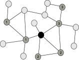
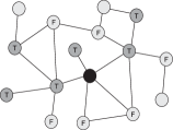
Among the several types of spreading in complex networks, we focus on those that can begin from a single node. The most common methods used in the literature are snowball (also called dilation), random walk, and contact process. An illustration of each method is shown in Figure 1.

(a)

(b)

(c)

Figure 1: Illustration of the spreading schemes after two iterations, considering the black node as seed. (a) Snowball spreading: the numbers 1 and 2 indicate the hierarchical levels. (b) Diffusion spreading: the numbers indicate the agent index that is executing the random walk. (c) Contact process: T represents nodes that accepted the contact, and F those that did not.

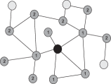
Snowball is a trivial spread where the subgraph is formed by the first n breadth-first searched nodes, forming the hierarchical levels of a given node. Because of its triviality, it is rarely used in practical problems, but more realistic methods tend to it on limiting cases, so we will start our analysis by this method. In our analysis, if the last hierarchical level can not be entirely covered, we randomly choose nodes from it so as to achieve the desired size of the extracted network.

On the random sample scheme, we start with R agents inside a unique node and let them simultaneously execute random walks through the network, the n first nodes visited by the agents are considered in the final subgraph. This method reduces to snowball when we let a large enough number of agents execute the walk. To show this, we call $P_{i}^{h}(T)$ the probability that a node i a geodesic distance h from the starting node receives a visit at iteration T, it is clear that

$$P_{i}^{h}(T<h)=0,$$

$$P_{i}^{h}(T=h)\propto 1-\left(1-\frac{1}{\left\{k\right\}}\right)^{R},$$

where $\left\{k\right\}$ is the product of the degree $k$ of each node in a shortest path between the starting node and i. If R is made large enough, $P_{i}^{h}(T=h)\rightarrow 1$ and we have again the snowball spreading.

The contact process, well known as epidemic process in the study of disease transmission, is done exactly like the susceptible-infected (SI) model SI_model (33), one of the simplest models of epidemics. In the initial state, all nodes of the network are in a susceptible state except one; then, for every connection between an infected and a susceptible node, the susceptible node turns to infected with a fixed probability p, which is equal for all connections. If $p=1$, a breadth-first transmission occurs and we have exactly the snowball scheme explained above.

Our method consists of performing S samplings of n nodes in an original network of size N, then we apply the centrality measurements to find each of the S initial nodes used to start the spreading process. Clearly, it is expected that the nodes with the higher centrality measurements have a better chance of being the seed, so we begin our analysis by verifying how much such measurements separate the seed from the other nodes and how well each one performs for the snowball spreading. Bear in mind that, from now on, spreading and sampling have the same meaning.

(a)

(b)

(c)

(d)

Figure 2: Frequency of occurrence for the four measurements considered, separated into seed nodes (diagonal hatch) and non-seed (checkered hatch and blue online) for 40000 nodes (400 subgraphs with size $n=100$). It is clear that, for all measurements, the seed has higher mean than the rest of the nodes. Note that the frequency of occurrence is normalized separately for the seed and non-seed nodes. The original network is an ER with $N=10000$.

III results and discussion

III.1 Source identification of a spreading process on artificial networks

(a) 100 nodes

(b) 1000 nodes

Figure 3: Histograms of the nodes with the highest centrality measurements with respect to the distance from the seed for ER (left) and BA (right) networks. The parameters are the same as those used in Figure 2.

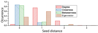
We start our analysis with an ER network with mean degree $<k>=6$ and size $N=10000$. We sampled 400 subgraphs with size $n=100$ each. For every subgraph, we applied the four centrality measurements discussed above and plotted the histogram of the data separating the values measured for the nodes used as seed and those that were not the seed. The results are shown in Figure 2.

The degree distribution of the seed nodes form a Poissonian shape bias (18) with mean degree $<k>\approx 6$, like the original network, but the distribution of the rest of the nodes has a scale free shape, which is expected considering that during the extraction process we create a small number of hubs that are close to the seed and many low-degree nodes in the last sampled level. From the histograms in Figure 2, it is clear that using the degree to find seeds is not a good choice, while the other three measurements have a smaller overlapping region between the two types of nodes, especially the betweenness that appears to give the best distinction for our purposes.

Figure 4: Betweenness (left) and Closeness (right) centrality as a function of the degree of the nodes for 400 sampled networks. The black points represent nodes used to start the sampling. The original network follows an ER model with $N=10000$ and $<k>=6$.

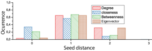
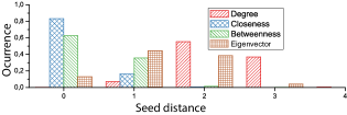
In Figure 3 we show the number of nodes with the highest centrality measurement divided by the number of extracted networks as a function of the distance from the seed; clearly, the ideal situation is when every node found has a distance zero from the seed, which is the seed itself. We see that, in the case of the ER model, even for a sampling of 1000 nodes, we get good results using closeness and betweenness, which is a consequence of the homogeneity of the network. The sampling breaks this homogeneity, as is clearly seen by the change in the degree distribution. Considering the strong topological bias present in the samples of the scale-free model (bear in mind that because we randomly choose the seeds, the majority of the samples were constructed from a very low-degree node, and such a node usually has a hub as a first or second neighbor) the method gives fair results for small extractions, but completely fails for larger ones.

Figure 5: Angular coefficients of the linear regression between log(betweenness) and log(degree), for networks extracted with different sizes. The original network was constructed using the BA model with $N=1000000$ nodes and $<k>=6$. For a given size, the mean was taken using 100 randomly selected seeds that originated a snowball sample. The vertical bars indicate the standard deviation.

(a)

(b)

Figure 6: Finding rate, represented in grayscale with contours as visual aid, of the seed as a function of extracted size and parameter r. The original network was generated using (6a) the BA procedure and (6b) the configuration model with $N=1000000$ and $<k>=6$. Note the different scale of r between the plots and the logarithmic scale of the extracted size.

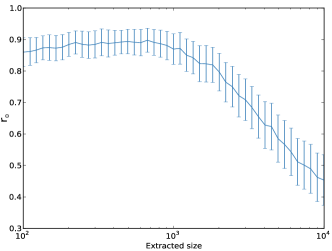
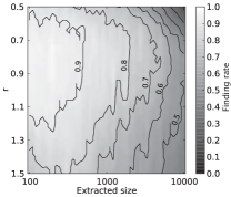
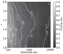
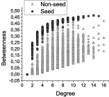
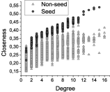
In order to improve the results, we refer to Figure 4, which shows the scatter plot of closeness and betweenness as a function of degree when considering an ER network, constructed using the same parameters of Figure 2, with seeds in black. We can see that, for low degree, the closeness tends to mix the two types of nodes, which is a property of the measurement and impossible to solve, but betweenness mixes low-degree seeds with high-degree normal nodes, a problem that can be solved, for example, by using equation 6. We now turn our attention to the unbiased betweenness defined by this equation, especially to the proper value of $r$. Starting with a BA network with $N=1000000$ nodes and $<k>=6$ we extracted, using snowball sampling, networks with sizes ranging from $n=100$ up to $n=10000$ (100 networks for each n) and fitted, using linear regression, the log-log plot of the relation betweenness versus degree. The obtained angular coefficients are shown in Figure 5; we expect that those values of $r_{0}$ are the best choice to define the unbiased betweenness at each extracted size, as it correctly eliminates the bias caused if the seed has low degree compared to other extracted nodes. To test this hypothesis, we plot in figure 6 the success of finding the seed (finding rate, defined as number of correct guesses divided by number of networks sampled) using the unbiased betweenness as a function of extracted size and parameter r. The original scale-free network was generated using the BA model (Figure 6a) and the configuration model with a power-law degree distribution with exponent $\gamma=3$ (Figure 6b). It is clear that the model used for the construction of the network is essential to the quality of the method in such a way that even the best choice for r was different between models. For the BA network, the finding rate was as high as 0.97 for some parameters, which is an almost perfect result, and the best choice for r is near the constant value of Figure 5.

(a)

(b)

Figure 7: Finding rate of the seed as a function of extracted size and parameter r. We used the configuration model to generate a network with (7a) $\gamma=2$ and (7b) $\gamma=4$ with $N=1000000$ and $<k>=6$. Again, note the different scale of r between the plots and the logarithmic scale of the extracted size.

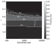
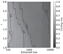
To test the influence of the exponent of the power-law degree distribution, the same simulation of Figure 6 was done for other two networks constructed using the configuration model with exponents $\gamma=2$ and $\gamma=4$, as shown in Figure 7. We found that larger values of $\gamma$ improve the results, while on very heterogeneous networks (small $\gamma$), we have too many nodes with high centrality and too strong fluctuations, leading to a failure of the methodology.

(a)

(b)

Figure 8: Finding rate of the seed as a function of extracted size and (8a) number of random walkers (represented by fac, see text for explanation) and (8b) contagion rate p of the contact process. The original network has $N=1000000$ and $<k>=6$.

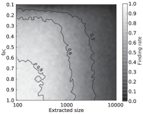
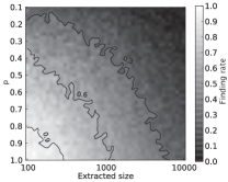
By using the unbiased betweenness with the empirical value $r=0.85$ suggested by the results, we can analyze the seed-finding success for the other two spreading techniches discussed above. In Figure 8a, we show the finding rate of the seed for networks extracted using random walkers with respect to different extracted sizes and number of agents, represented by fac defined as

$$\text{number\, of\, agents}=\text{fac}\times\text{extracted\, size}$$

It is clear that, even for a small number of agents, which creates a network composed of many chains (a sequence of connected nodes with degree two), the method still gives fair results. We repeated the procedure for contact processes with varying contagion rates, shown in Figure 8b, where we see that the procedure still gives good results.

III.2 Source identification in a real network

(a)

Figure 9: Finding rate of the seed as a function of extracted size and parameter r. The original network represents the exchange of emails between members of the University Rovira i Virgili.

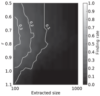
At last, we applied the unbiased betweenness with $r=0.85$ described above to the email network of the members of the University Rovira i Virgili real_network (27), where each email address becomes a node and a connection occurs if address A has sent a message to B and B has sent an email to A. The giant component of the network contains 1133 nodes and 10902 edges, so we extracted a number of nodes ranging from 100 to 1000 using snowball spread beginning from randomly selected seeds. The obtained results are shown in Figure 9. We can see that, even for a real network, it is possible to obtain a hint about the location of the source, if the extracted (or infected) network is small compared to the original.

IV Conclusion

It is clear that the identification of the seed node has great importance for the characterization of a network originated from a spreading process. Our purpose was to devise a method that could find this seed node with the highest success rate possible. To do so, we utilized four centrality measurements, which provide information about the relative importance of a node, and applied them to diverse networks extracted from ER and scale-free models, as well as an email network. We found that the seed node has, in general, higher centrality than the other nodes, so that finding the node with the highest potential of access allows the identification of the source of the network. When applying a single measurement, the obtained results had success rates higher than 0.8 for large ER networks and fairly good values for scale-free structures. We showed that a simple combination of those measurements offers a remarkable result of more than 0.95 success rate for small scale-free networks, considering the high heterogeneity of the network and that the result strongly depends on the data being analyzed, as indicated by the different results obtained between the BA, the configuration model, and the email network. Finally, we compared the success rate for two other spreading schemes, namely, random sample and contact process, with varying number of walkers and contagion rate, showing that the method works very well if the dynamic is close enough to a snowball spreading and gives fairly good results to intermediate parameters.

As said before, it may be possible to improve the results by combining different centrality measurements with pattern recognition methods. Also, we could devise a method of comparing the centrality of the original network with that of the sampled one, which is an interesting idea, but would require us to entirely know the original network, which is not always possible. Finally, the method could be applied to a network containing information about a real spreading process.