Technical Report No. 1002
Department of Statistics, University of Toronto
Covariance-Adaptive Slice Sampling

Abstract

We describe two slice sampling methods for taking multivariate steps using the crumb framework. These methods use the gradients at rejected proposals to adapt to the local curvature of the log-density surface, a technique that can produce much better proposals when parameters are highly correlated. We evaluate our methods on four distributions and compare their performance to that of a non-adaptive slice sampling method and a Metropolis method. The adaptive methods perform favorably on low-dimensional target distributions with highly-correlated parameters.

1 Introduction

Markov Chain Monte Carlo methods often perform poorly when parameters are highly correlated. Our goal has been to develop MCMC methods that work well on such distributions without requiring prior knowledge about the distribution or extensive tuning runs.

Slice sampling (Neal,, 2003) is an auxiliary-variable MCMC method based on the idea of drawing points uniformly from underneath the density surface of a target distribution. If one discards the density coordinate from the sample, the resulting marginal distribution is the target distribution.

This document presents two samplers in the “crumb” framework (Neal,, 2003, §5.2), a general framework for slice sampling methods that take multivariate steps. Unlike many MCMC samplers, they perform well when the target distribution has highly correlated parameters. These methods can improve on univariate slice sampling in the same way Metropolis with a properly chosen multivariate proposal distribution can improve on Metropolis with a spherical proposal distribution and on Metropolis updates of one coordinate at a time.

2 Multivariate Steps in the Crumb Framework

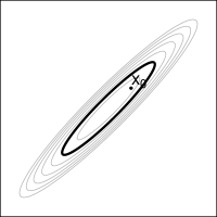
(a)	(b)

Figure 1: (a) Contours of a target distribution. (b) A slice, $S_{y_{0}}$, and the current target component, $x_{0}$.

This section describes the crumb framework for taking multivariate steps in slice sampling. The overall goal is to sample from a target distribution, such as the one with log-density contours shown in figure 1(a). The dimension of the target distribution’s parameter space is denoted by $p$. (The example in the figure has $p=2$.) The state space of the Markov chain for slice sampling has dimension $p+1$, of which $p$ correspond to the target distribution and one to the current slice level.

Slice sampling alternates between sampling the target coordinates and the density coordinate. Let $f(x)$ be proportional to the density function of the target distribution, and let $(x_{0},y_{0})$ be the current state in the augmented sample space, where $x_{0}\in\mathbb{R}^{p}$ and $y_{0}\in\mathbb{R}$. To update the density component, $y_{0}$, we sample uniformly from $[0,f(x_{0})]$. Updating the target component, $x_{0}$, is more difficult. Let $S_{y_{0}}$ be the slice through the distribution at level $y_{0}$:

$$S_{y_{0}}=\{x:f(x)\geq y_{0}\}$$ (1)

The set $S_{y_{0}}$ is outlined by a thick line in figure 1(b). The difficulty in updating the target component is that we rarely have an analytic expression for the boundary of $S_{y_{0}}$, which may not even be a connected curve, so we cannot sample uniformly from $S_{y_{0}}$ as we would like to. The methods of this document instead perform updates that leave the uniform distribution on $S_{y_{0}}$ invariant, leaving the resulting chain with the desired stationary distribution.

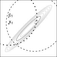
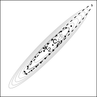
(a)	(b)

Figure 2: (a) The first crumb, $c_{1}$, and a proposal, $x_{1}$. The distribution of $c_{1}$ is shown as dashed. The distribution of $x_{1}$ is shown as dotted. In this figure and subsequent ones, probability distributions in a two-dimensional space are represented by ellipses such that a uniform distribution over the ellipse has the same mean and covariance as the represented distribution. This method allows multiple distributions to be drawn in the same plot. (b) The second crumb, $c_{2}$, and a proposal, $x_{2}$. The distribution of $c_{2}$ is shown as dashed. The distribution of $x_{2}$ is shown as dotted. The distribution for $c_{2}$ has been updated using the method described in section 4.

These methods begin by sampling a “crumb,” $c_{1}$, from a distribution that depends on $x_{0}$, then drawing a proposal, $x_{1}$, from the distribution of points that could have generated $c_{1}$, treating the crumb as data and $x_{0}$ as an unknown. An example crumb and proposal are drawn in figure 2(a), with the distribution of $c_{1}$ shown as a dashed line and the distribution of $x_{1}$ shown as a dotted line.

If $x_{1}$ were inside $S_{y_{0}}$, we would accept it as the new value for the target component of the state. In figure 2(a), it is not, so we draw a new crumb, $c_{2}$, and draw a new proposal, $x_{2}$, from the distribution of $x_{0}$ given both $c_{1}$ and $c_{2}$ as data. This is plotted in figure 2(b). While the distribution of proposed moves is determined by the crumbs and their distributions, we can choose the distribution of the crumbs arbitrarily, using the densities and gradients at rejected proposals if we desire.

In the example of figure 2(b), $x_{2}$ is in $S_{y_{0}}$, so we accept $x_{2}$ as the new target component. If it were not, we would keep drawing crumbs, adapting their distributions so that the proposal distribution would be as close as possible to uniform sampling over $S_{y_{0}}$, and metaphorically following these crumbs back to $x_{0}$ by drawing proposals from the distribution of $x_{0}$ conditional on having observed the crumbs (Grimm and Grimm,, 2008).

Neal, (2003, §5.2) has more information on the crumb framework, including a proof that methods in this framework leave the target distribution invariant.

3 Overview of Adaptive Gaussian Crumbs

We now specialize the crumb framework to Gaussian crumbs and proposals, using log densities at proposals and their gradients to choose the crumb covariances. Without violating detailed balance, the crumb distribution can depend on these log densities and gradients. We assume that while computing the log density at a proposal, we can compute its gradient with minimal additional cost.

Ideally, the proposal distribution would be a uniform distribution over $S_{y_{0}}$. To approximate uniform sampling over $S_{y_{0}}$, we attempt to draw a sequence of crumbs that results in a Gaussian proposal distribution with the same covariance as a uniform distribution over the slice.

In both adaptive methods discussed in this document, the first crumb has a multivariate Gaussian distribution:

$$c_{1}\sim N(x_{0},W_{1}^{-1})\quad\text{where $W_{1}=\sigma_{c}^{-2}I$}$$ (2)

The standard deviation of the initial crumb, $\sigma_{c}$, is the only tuning parameter for either method that is modified in normal use. The distribution for $x_{0}$ given $c_{1}$ is a Gaussian with mean $c_{1}$ and precision matrix $W_{1}$, so we draw a proposal from this distribution:

$$x_{1}\sim N(c_{1},W_{1}^{-1})$$ (3)

If $f(x_{1})$ is at least $y_{0}$, then $x_{1}$ is inside the slice, so we accept $x_{1}$ as the target component of the next state of the chain. This update leaves the density component, $y_{0}$, unchanged, though it is usually forgotten after a proposal is accepted, anyway.

When the proposal is not in the slice, we choose a different covariance matrix, $W_{k+1}$, for the next crumb, so that the covariance of the next proposal will look more like that of uniform sampling over $S_{y_{0}}$. The two methods proposed in this document differ in how they make that choice; sections 4 and 5 describe the details.

After sampling $k$ crumbs from Gaussians with mean $x_{0}$ and precision matrices $(W_{1},\ldots,W_{k})$, the distribution for the $k$th proposal (the posterior for $x_{0}$ given the crumbs) is:

$$x_{k} \sim N(\bar{c}_{k},\Lambda_{k}^{-1})$$ (4)

$$\text{where}\;\Lambda_{k} =W_{1}+\cdots+W_{k}$$ (5)

$$\text{and}\;\bar{c}_{k} =\Lambda_{k}^{-1}(W_{1}c_{1}+\cdots+W_{k}c_{k})$$ (6)

If $x_{k}\in S_{y_{0}}$—that is, if $f(x_{k})\geq y_{0}$—we accept $x_{k}$ as the target component. Otherwise, we must choose a covariance for the distribution of $(k+1)$th crumb, draw a new proposal, and repeat until a proposal is accepted.

4 First Method: Matching the Slice Covariance

In the method described in this section, we attempt to find $W_{k+1}$ so that the $(k+1)$th proposal distribution has the same conditional variance as uniform sampling from $S_{y_{0}}$ in the direction of the gradient of $\log f(\cdot)$ at $x_{k}$. This gradient is a good guess at the direction in which the proposal distribution is least like $S_{y_{0}}$. Figure 3(a) shows an example of this. We plotted the gradients of the log density at thirty points drawn from the same distribution (shown as a dotted line) as a rejected proposal; most of these gradients point in the direction where the proposal variance is least like the slice. Generally, in an ill-conditioned distribution, these gradients do not point towards the mode, they point towards the nearest point on the slice. (In a well-conditioned distribution, the directions to the mode and to the nearest point on the slice will be similar.)

4.1 Choosing Crumb Covariances

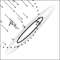
(a)	(b)	(c)

Figure 3: (a) shows gradients at thirty points drawn from the first proposal distribution (shown as a dotted line). These gradients tend to point towards the slice (shown as a thick line). (b) shows a parabolic cut through the log-density surface that goes through a rejected proposal, $x_{1}$, in the direction of the gradient at $x_{1}$, shown as an arrow. $u_{1}$ is a point on the cut defined by equation 12. (c) adds a parabolic cut through the mode in the same direction. These two parabolas have approximately the same second derivative. The distance between the two arms of the second parabola when the vertical coordinate is equal to $\log y_{0}$ is shown as a double-ended arrow, equal to $d$ in equation 16.

To compute $W_{k+1}$, we will estimate the second derivative of the target distribution in the direction of the gradient, assuming the target distribution is approximately locally Gaussian. Consider the (approximately) parabolic cut through the log-density surface in figure 3(b), which has the equation:

$$\ell=-\frac{1}{2}\kappa t^{2}+\beta t+\gamma$$ (7)

$t$ is a parameter that is zero at $x_{k}$ and increases in the direction of the gradient; $\kappa$, $\beta$, and $\gamma$ are unknown constants we wish to estimate. The coefficient $-\frac{1}{2}$ is arbitrary; this choice makes $\kappa$ equal to the negative of the second derivative of the parabola. We already had to compute $f(x_{k})$ so that we could determine whether $x_{k}$ was in $S_{y_{0}}$; we assume that $\nabla\log f(x_{k})$ was computed simultaneously. To fix two degrees of freedom of the parabola, we plug these quantities into equation 7 and its derivative with respect to $t$:

$$\log f(x_{k}) =-\frac{1}{2}\kappa\cdot 0^{2}+\beta\cdot 0+\gamma=\gamma$$ (8)

$$\lVert\nabla\log f(x_{k})\rVert =-\kappa\cdot 0+\beta=\beta$$ (9)

We still have one degree of freedom left, so we must evaluate $\log f(\cdot)$ at another point on the parabola. We choose a point as far away from $x_{k}$ as $c_{k}$ is, hoping that this distance is within the range where the distribution is approximately Gaussian. Let $\delta$ be this distance:

$$\delta=\lVert x_{k}-c_{k}\rVert$$ (10)

Let $g$ be the normalized gradient at $x_{k}$:

$$g=\frac{\nabla\log f(x_{k})}{\lVert\nabla\log f(x_{k})\rVert}$$ (11)

Then, the point $u_{k}$ is defined to be $\delta$ away from $x_{k}$ in the direction $g$:

$$u_{k}=x_{k}+\delta\cdot g$$ (12)

In equation 7, $u_{k}$ corresponds to $t=\delta$. We evaluate the density at $u_{k}$ to fix the parabolic cut’s third degree of freedom, and plug this into equation 7:

$$\log f(u_{k})=-\frac{1}{2}\kappa\delta^{2}+\beta\delta+\gamma$$ (13)

Solving equations 8, 9, and 13 for $\kappa$ gives:

$$\kappa=-\frac{2}{\delta^{2}}\bigl{(}\log f(u_{k})-\log f(x_{k})-\lVert\nabla\log f(x_{k})\rVert\cdot\delta\bigr{)}$$ (14)

We can now use $\kappa$ to approximate the conditional variance in the direction $g$. If the Hessian is locally approximately constant, as it is for Gaussians, a cut through the mode in the direction of $\nabla\log f(x_{k})$ would have the same second derivative as the cut through $x_{k}$. This second parabola, shown in figure 3(c), has the equation:

$$\ell=-\frac{1}{2}\kappa t^{2}+M$$ (15)

$M$ is the log density at the mode. We set $t=0$ at the mode, so there is no linear term. For now, assume $f(\cdot)$ is unimodal and that $M$ was computed with the conjugate gradient method (Nocedal and Wright,, 2006, ch. 5) or some other similar procedure before starting the Markov chain. We solve equation 15 for the parabola’s diameter $d$ at the level of the current slice, $\log y_{0}$, shown as a doubled-ended arrow in figure 3(c):

$$d=\sqrt{\frac{8(M-\log y_{0})}{\kappa}}$$ (16)

Since the distribution of points drawn from an ellipsoidal slice, conditional on their lying on that particular one-dimensional cut, is uniform with length $d$, the conditional variance in the direction of the gradient at $x_{k}$ is:

$$\sigma^{2}_{k+1}=\frac{d^{2}}{12}=\frac{2}{3}\cdot\frac{M-\log y_{0}}{\kappa}$$ (17)

With this variance, we can construct a crumb precision matrix that will lead to the desired proposal precision matrix. We want to draw a crumb $c_{k+1}$ so that the posterior of $x_{0}$ given the $k$ crumbs has a variance equal to $\sigma_{k+1}^{2}$ in the direction $g$. Using equation 5, the precision of the proposal given these crumbs is:

$$\Lambda_{k+1}=\Lambda_{k}+W_{k+1}$$ (18)

If we multiply both sides of equation 18 by $g^{T}$ on the left and $g$ on the right, the left side is the conditional precision in the direction $g$.

$$g^{T}\Lambda_{k+1}g=g^{T}\bigl{(}\Lambda_{k}+W_{k+1}\bigr{)}g$$ (19)

We would like to choose $W_{k+1}$ so that this conditional precision is $\sigma_{k+1}^{-2}$, so we replace the left hand side of equation 19 with that:

$$\sigma_{k+1}^{-2}=g^{T}\bigl{(}\Lambda_{k}+W_{k+1}\bigr{)}g$$ (20)

As will be discussed in section 4.3, computation will be particularly easy if we choose $W_{k+1}$ to be a scaled copy of $\Lambda_{k}$ with a rank-one update, so we choose $W_{k+1}$ to be of the form:

$$W_{k+1}=\theta\Lambda_{k}+\alpha gg^{T}$$ (21)

$\alpha$ and $\theta$ are unknown scalars. $\theta$ controls how fast the precision as a whole increases. If we would like the variance in directions other than $g$ to shrink by $9/10$, for example, we choose $\theta=1/9$. Since $\theta$ is constant, there will be exponentially fast convergence of the proposal covariance in all directions, which allows quick recovery from overly diffuse initial crumb distributions. For this method, $\theta$ is not a critical choice; $\theta=1$ is reasonable. Substituting equation 21 into equation 20 gives:

$$\sigma_{k+1}^{-2}=g^{T}\bigl{(}\Lambda_{k}+\theta\Lambda_{k}+\alpha gg^{T}\bigr{)}g$$ (22)

Noting that $g^{T}g=1$, we solve for $\alpha$, and set:

$$\alpha=\max\{\sigma_{k+1}^{-2}-(1+\theta)g^{T}\Lambda_{k}g,0\}$$ (23)

$\alpha$ is restricted to be positive to guarantee positive definiteness of the crumb covariance. (By choosing $\theta$ simultaneously, we could perhaps encounter this restriction less frequently, but we have not explored this.) Once we know $\alpha$, we then compute $W_{k+1}$ using equation 21.

The resulting crumb distribution is:

$$c_{k+1}\sim N(x_{0},W_{k+1}^{-1})$$ (24)

After drawing such a crumb, we draw a proposal according to equations 4 to 6, accepting or rejecting depending on whether $f(x_{k+1})\geq y_{0}$, drawing more crumbs and adapting until a proposal is accepted.

4.2 Estimating the Density at the Mode

We now modify the method to remove the restriction that the target distribution be unimodal and remove the requirement that we precompute the log density at the mode. Estimating $M$ each time we update $x_{0}$ instead of precomputing it allows $M$ to take on values appropriate to local modes. Since the proposal distribution only approximates the slice even in the best of circumstances, it is not essential that the estimate of $M$ be particularly good.

To estimate $M$, we initialize $M$ to the slice level, $\log y_{0}$, before drawing the first crumb. Then, every time we fit the parabola described by equation 7, we update $M$ to be the maximum of the current value of $M$ and the estimated peak of the parabola. As more crumbs are drawn, $M$ becomes a better estimate of the local maximum. We could also use the values of the log density at rejected proposals and at the $\{u_{k}\}$ to bound $M$, but if the log density is locally concave, the log densities at the peaks of the parabola will always be larger than these values.

4.3 Efficient Computation of the Crumb Covariance

This section describes a method for using Cholesky factors of precision matrices to make implementation of the covariance-matching method of section 4.1 efficient. If implemented naively, the method of section 4.1 would use $O(p^{3})$ operations when drawing a proposal with equations 4 and 6. We would like to avoid this. One way is to represent $W_{k}$ and $\Lambda_{k}$ by their upper-triangular Cholesky factors $F_{k}$ and $R_{k}$, where $F_{k}^{T}F_{k}=W_{k}$ and $R_{k}^{T}R_{k}=\Lambda_{k}$.

First, we must draw proposals efficiently. If $z_{1}$ and $z_{2}$ are $p$-vectors of standard normal variates, we can replace the crumb and proposal draws of equations 24 and 4 with:

$$c_{k} =x_{0}+F_{k}^{-1}z_{1}$$ (25)

$$x_{k} =\bar{c}_{k}+R_{k}^{-1}z_{2}$$ (26)

Since Cholesky factors are upper-triangular, evaluation of $F_{k}^{-1}z_{1}$ and $R_{k}^{-1}z_{2}$ by backward substitution takes $O(p^{2})$ operations.

We must also update the Cholesky factors efficiently. We replace the updates of $W_{k}$ and $\Lambda_{k}$ in equations 21 and 18 with:

$$F_{k+1} =\operatorname{chud}(\sqrt{\theta}R_{k},\sqrt{\alpha}g)$$ (27)

$$R_{k+1} =\operatorname{chud}(\sqrt{1+\theta}R_{k},\sqrt{\alpha}g)$$ (28)

Here, $\operatorname{chud}(R,v)$ is the Cholesky factor of $R^{T}R+vv^{T}$. The function name is an abbreviation for “Cholesky update.” It can be computed with the LINPACK routine DCHUD, which uses Givens rotations to compute the update in $O(p^{2})$ operations (Dongarra et al.,, 1979, ch. 10).

Finally, we would like to compute the proposal mean efficiently. We do this by keeping a running sum of the un-normalized crumb mean (the parenthesized expression in equation 6), which we will represent by $\bar{c}_{k}^{*}$. Define:

$$\bar{c}_{k}^{*} =W_{1}c_{1}+\cdots+W_{k}c_{k}$$ (29)

$$=\bar{c}_{k-1}^{*}+W_{k}c_{k}$$ (30)

$$=\bar{c}_{k-1}^{*}+F_{k}^{T}F_{k}c_{k}$$ (31)

Then, using forward and backward substitution, we can compute the normalized crumb mean, $\bar{c}_{k}$, as:

$$\bar{c}_{k}=R_{k}^{-1}R_{k}^{-T}\bar{c}_{k}^{*}$$ (32)

This way, we can compute $\bar{c}_{k}$ in $O(p^{2})$ operations and do not need to save all the crumbs and crumb covariances.

With these changes, the resulting algorithm is numerically stable even with ill-conditioned target distributions. Each crumb and proposal draw takes $O(p^{2})$ operations. Figure 4 shows pseudocode for this method.

Slice Sampling with Covariance Matching

⬇

Initialize $N$, $f$, $x_{0}\in\mathbb{R}^{p}$, $\sigma_{c}$, and $\theta$.

$X\leftarrow(\,)$

repeat $N$ times:

$M\leftarrow\log f(x_{0})$

$e\leftarrow\operatorname{\text{draw from}}\operatorname{Exponential}(1)$

$\tilde{y}_{0}\leftarrow M-e$

$R\leftarrow\sigma_{c}^{-1}I$

$F\leftarrow\sigma_{c}^{-1}I$

$\bar{c}^{*}\leftarrow 0$

repeat until a proposal is accepted:

$z\leftarrow\operatorname{\text{draw from}}N_{p}(0,I)$

$c\leftarrow x_{0}+F^{-1}z$

$\bar{c}^{*}\leftarrow\bar{c}^{*}+F^{T}Fc$

$\bar{c}\leftarrow R^{-1}R^{-T}\bar{c}^{*}$

$z\leftarrow\operatorname{\text{draw from}}N_{p}(0,I)$

$x\leftarrow\bar{c}+R^{-1}z$

$\tilde{y}\leftarrow\log f(x)$

if $\tilde{y}\geq\tilde{y}_{0}$:

proposal accepted, break

end (if)

$G\leftarrow\nabla\log f(x)$

$g\leftarrow G/\lVert G\rVert$

$\delta\leftarrow\lVert x-c\rVert$

$u\leftarrow x+\delta g$

$\ell_{u}\leftarrow\log f(u)$

$\kappa\leftarrow-2\delta^{-2}\left(\ell_{u}-\tilde{y}-\delta\lVert G\rVert\right)$

$\ell_{x,u}\leftarrow\frac{1}{2}\frac{\lVert G\rVert^{2}}{\kappa}+\tilde{y}$

$M\leftarrow\max\left\{M,\ell_{x,u}\right\}$

$\sigma^{2}\leftarrow\frac{2}{3}\frac{M-\tilde{y}_{0}}{\kappa}$

$\alpha\leftarrow\max\left\{0,\sigma^{-2}-(1+\theta)g^{T}R^{T}Rg\right\}$

$F\leftarrow\operatorname{chud}\left(\sqrt{\theta}R,\sqrt{\alpha}g\right)$

$R\leftarrow\operatorname{chud}\left(\sqrt{1+\theta}R,\sqrt{\alpha}g\right)$

end (repeat)

append $x$ to $X$.

$x_{0}\leftarrow x$

end (repeat)

return X

Figure 4: This figure shows the adaptive algorithm of section 4. The variables are mostly the same as in the text, with a few exceptions: To avoid underflow, we set $\tilde{y}=\log y$ and $\tilde{y}_{0}=\log y_{0}$; see Neal, (2003, §4) for discussion. The $k$ subscript is dropped since there is no need to keep copies of the values from any but the most recent iteration. The variable $\ell_{x,u}$ indicates the peak of the parabolic cut through $x$ and $u$; $N$ indicates the number of samples to draw. The generated samples are stored in the ordered set $X$.

5 Second Method: Shrinking the Rank of the Crumb Covariance

The method of section 4 attempts to adapt the crumb distribution so that the proposal distribution matches the shape of the slice. However, it often can’t due to positive-definiteness constraints, requiring the $\max\{\cdot,\cdot\}$ operation in equation 23. Even when it can perform the adaptation, it may not be appropriate if the underlying distribution is not approximately Gaussian.

This section describes a different method, also based on the framework of section 3. Instead of attempting to match the conditional variance in the direction of the gradient, it just sets it to zero. This is reasonable in that the gradient at a proposal probably points in a direction where the variance is small, so it is more efficient to move in a different direction.

With this method, the crumb covariance is zero in some directions and spherically symmetric in the rest, so its simplest representation is the pair $(w,J)$, where $J$ is a matrix of orthonormal columns of directions in which the conditional variance is zero, and $w^{2}$ is the variance in the other directions.

Define $P(J,v)$ to be the function that returns the component of vector $v$ orthogonal to the columns of $J$:

$$P(J,v)=\begin{cases}v-JJ^{T}v&\quad\text{if $J$ has at least one column}\\ v&\quad\text{if $J$ has no columns}\end{cases}$$ (33)

For simplicity of computation, since the crumbs are located in a common subspace with $x_{0}$, this method will consider the origin to be at $x_{0}$ except when calling $f(\cdot)$, which is provided by the user, and when returning samples to the user. Each crumb is drawn by:

$$c_{k}=\sigma_{c}\,P(J,z)\qquad\text{where $z\sim N_{p}(0,I)$}$$ (34)

When the first crumb is drawn, $J$ has no columns, so $P(J,z)=z$ and the first crumb has the distribution specified in section 3.

Given $k$ crumbs and the covariances of their distributions, we know that $x_{0}$ must lie in the intersection of the subspaces of their covariances. Since the subspace $c_{j}$ is drawn from contains the subspace $c_{k}$ is drawn from when $k>j$, this is equivalent to saying that $x_{0}$ must lie in the subspace of $c_{k}$’s covariance, the orthogonal complement of $J$. So, the precision of the posterior for $x_{0}$ in the direction of columns of $J$ is infinite. It is equal to $k\sigma_{c}^{-2}$ in all other directions, since there are $k$ crumbs, each with spherical variance equal to $\sigma_{c}^{2}$ in the subspace they were drawn in. The mean of the proposal distribution (with origin $x_{0}$) is the projection of:

$$\bar{c} =\frac{\sigma_{c}^{-2}c_{1}+\cdots+\sigma_{c}^{-2}c_{k}}{k\sigma_{c}^{-2}}$$

$$=k^{-1}\left(c_{1}+\cdots+c_{k}\right)$$ (35)

Therefore, to draw a proposal, we draw a vector of standard normal variates, project it into the orthogonal complement of $J$, scale by $\sigma_{c}/\sqrt{k}$, and add $\bar{c}$, also projected into the orthogonal complement of $J$. With the original origin, the proposal is:

$$x_{k}=x_{0}+P(J,\bar{c})+(\sigma_{c}/\sqrt{k})\cdot P(J,z)\qquad\text{where $z\sim N_{p}(0,I)$}$$ (36)

If the proposal is in the slice (that is, if $f(x_{k})\geq y_{0}$), we accept it. Otherwise, we adapt the crumb distribution. If $J$ has $p-1$ columns, we can’t add any more without the crumb covariance having a rank of zero, so we do not adapt in that case. Otherwise, we add a single new column in the direction of $\nabla\log f(x_{k})$, projected into the directions not already spanned by $J$, which we denote by $g^{*}$. Thus, the new value of $J$ would be:

$$J_{k+1} =\left[J_{k}\quad\frac{g^{*}}{\lVert g^{*}\rVert}\right]$$ (37)

$$\text{where}\quad g^{*} =P\left(J_{k},\nabla\log f(x_{k})\right)$$ (38)

To prevent meaningless adaptations, we only perform this operation when the angle between the gradient and its projection into the nullspace of $J$ is less than $60^{\circ}$. Equivalently, we only adapt when:

$$\frac{{g^{*}}^{T}\nabla\log f(x_{k})}{\lVert g^{*}\rVert\,\lVert\nabla\log f(x_{k})\rVert}>\frac{1}{2}$$ (39)

After possibly updating $J$, we draw another crumb and proposal, repeating until a proposal is accepted. The method of this section is summarized in figure 5.

Crumbs with Shrinking-Rank Covariance

⬇

Initialize $N$, $f$, $x_{0}\in\mathbb{R}^{p}$, and $\sigma_{c}$.

$X\leftarrow(\,)$

repeat $N$ times:

$e\leftarrow\operatorname{\text{draw from}}\operatorname{Exponential}(1)$

$\tilde{y}_{0}\leftarrow\log f(x_{0})-e$

$J\leftarrow[\;]$

$k\leftarrow 0$

$\bar{c}\leftarrow 0$

repeat until a proposal is accepted:

$k\leftarrow k+1$

$z\leftarrow\operatorname{\text{draw from}}N_{p}(0,I)$

$c\leftarrow\sigma_{c}z$

$\bar{c}\leftarrow k^{-1}\bigl{(}(k-1)\bar{c}+c\bigr{)}$

$z\leftarrow\operatorname{\text{draw from}}N_{p}(0,I)$

$x\leftarrow x_{0}+P\left(J,\bar{c}+\frac{\sigma_{c}}{\sqrt{k}}z\right)$

if $\log f(x)\geq\tilde{y}_{0}$:

proposal accepted, break

end (if)

if $J$ has less than $p-1$ columns:

$g^{*}\leftarrow P(J,\nabla\log f(x))$

if ${g^{*}}^{T}\nabla\log f(x)>\frac{1}{2}\lVert g^{*}\rVert\,\lVert\nabla\log f(x)\rVert$:

$J\leftarrow[\;J\quad g^{*}/\lVert g^{*}\rVert\;]$

end (if)

end (if)

end (repeat)

append $x$ to $X$.

$x_{0}\leftarrow x$

end (repeat)

return X

Figure 5: The adaptive algorithm of section 5. This differs from that section in that the projection into the nullspace of $J$ is delayed until drawing a proposal, reducing the number of matrix products computed.

A variation on the method (which we use in the implementation tested in section 7) shrinks the crumb standard deviation in the nonzero directions, $\sigma_{c}$, by a constant factor each time a crumb is drawn; section 7 uses 0.9. This results in exponentially falling proposal variance, which, as described in section 4.1, allows large initial crumb variances to be used.

6 Procedure for Evaluation

Figures 6 and 7 demonstrate the performance of the methods described in this document. Figure 6 demonstrates the performance of four samplers on a Gaussian distribution (to be described in section 7). It contains two graphs, one for each of two figures of merit. The top graph plots log density function evaluations per independent sample against a tuning parameter. The bottom graph plots processor-seconds per independent sample against a tuning parameter. For both figures of merit, smaller is better.

Each of the four panes in each graph contains data from a single sampler, with each point representing a run with a specific tuning parameter. The tuning parameter for each sampler has the same scale; the sampler initially attempts to take steps roughly that size.

Both figures of merit require us to determine the correlation length, the number of correlated samples equivalent to an independent sample. For the runs done here, an AR(1) model captures the necessary structure. For each parameter, we fit the following model:

$$X_{t}=E(X_{t})+\pi\cdot X_{t-1}+a_{t}$$ (40)

where $a_{t}$ is a noise process. Then, the number of samples equivalent to a single independent sample is:

$$\tau=\frac{\operatorname*{var}(a_{t})}{\operatorname*{var}(X_{t})\cdot(1-\pi)^{2}}$$ (41)

This formula is based on the effectiveSize function in CODA (Plummer et al.,, 2006), which uses the spectral approach of Heidelberger and Welch, (1981). Wei, (2006, pp. 276–278) has a more in-depth discussion of the spectrum of AR processes. To estimate a correlation length for a multivariate distribution, we take the largest estimated correlation length of each of its parameters. This is not valid in general, but is an acceptable approximation for this experiment.

Most chains are displayed with a circle indicating an estimate of the figure of merit, with a line indicating a nominal 95% confidence interval. The intervals are based on normality of the increments of the AR(1) process, so they should be viewed as a lower bound on the uncertainty of the point estimates. Chains whose figures are plotted as question marks were estimated as having an effective sample size of less than four.

Figure 7 contains information on four different samplers. The panes of figure 7 are similar to those of figure 6, and each is labeled with the distribution and the sampler the chains in that pane come from. The columns of panes correspond to samplers; the rows of panes correspond to distributions. By reading across, one can see how different samplers perform on a given distribution. By reading down, one can see how the performance of a given sampler varies from distribution to distribution.

Every chain has 150,000 samples. In general, the chain length does not affect the results; we will point out exceptions to this.

7 Results of Evaluation

We simulated four samplers on four distributions for twelve different tuning parameters each. The samplers we considered are:

• Covariance-Matching: This is the method described in section 4. The tuning parameter is $\sigma_{c}$.

• Shrinking-Rank: This is the method described in section 5. The tuning parameter is $\sigma_{c}$.

• Non-Adaptive Crumbs: This is a non-adaptive variant of the general method of section 3. It is like the method of section 5, but never shrinks rank. However, like that method, it scales the crumb standard deviation down by $0.9$ after each proposal. The tuning parameter is $\sigma_{c}$.

• Metropolis (with Trials): This method is a Metropolis sampler that uses trial runs to automatically determine a suitable Gaussian proposal distribution. The tuning parameter specifies the standard deviation of the proposal distribution for the first trial run.

The distributions we considered are:

• $N_{4}(\rho=0.999)$: This is a four-dimensional Gaussian with highly-correlated parameters. The marginal variances for each parameter are one; each parameter has a correlation of $0.999$ with each other parameter. The covariance matrix has a condition number of about 2900 and is not diagonal.

• $N_{4}(\rho=-0.3329)$: This is a four-dimensional Gaussian with negatively-correlated parameters. The marginal variances for each parameter are one, and each parameter has a correlation of $-0.3329$ with each other parameter. The covariance has a condition number of about 2900, like $N_{4}(\rho=0.999)$, but instead of one large eigenvalue and three small ones, this distribution has one small eigenvalue and three large ones.

• Eight Schools: This is a multilevel model in ten dimensions, consisting of eight group means and hyperparameters for their mean and variance. It comes from Gelman et al., (2004, pp. 138–145).

• Ten-Component Mixture: This is a ten-component Gaussian mixture in $\mathbb{R}^{10}$. Each mode is a spherically symmetric Gaussian with unit variance. The modes are uniformly distributed on a hypercube with edge-length ten.

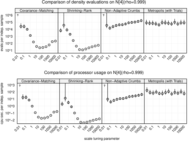
Figure 6: The performance of four MCMC samplers on $N_{4}(\rho=0.999)$. See section 6 for a description of the graphs and section 7 for discussion.

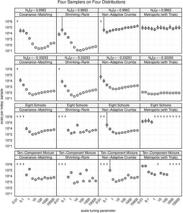
Figure 7: The performance of four MCMC samplers on four distributions. See section 6 for a description of the graph and section 7 for discussion.

By comparing the top and bottom graphs of figure 6, we see that for $N_{4}(\rho=0.999)$, processor time and number of density evaluations tell the same story. The plots of function evaluations and the plots of processor time are nearly identical except for their vertical scales. This is true of the other distributions as well, so we do not repeat the processor-time plots for the others.

Figure 6 (and the identical first row of figure 7) shows the performance of the four methods on a highly-correlated four-dimensional Gaussian, $N_{4}(\rho=0.999)$. Both adaptive slice sampling methods perform well once the tuning parameter is at least the same order as the standard deviation of the target distribution. This hockey-stick performance curve is characteristic of slice sampling methods. The non-adaptive slice sampling method always takes steps of the order of the smallest eigenvalue once its tuning parameter is at least that large, so its performance is bad, but after this threshold, its performance does not depend much on the tuning parameter. The Metropolis sampler also fails to capture the shape of the distribution, a result that depends more on chain length. Had the chain been longer, the preliminary runs the sampler uses to estimate a proposal distribution might have worked better, leading to average performance comparable to the adaptive slice samplers.

The second row of figure 7 shows sampler performance on a similar but negatively correlated four-dimensional Gaussian, $N_{4}(\rho=-0.3329)$. The adaptive slice sampling methods continue to perform well on this distribution, and the non-adaptive sampler improves somewhat. The Metropolis sampler improves a great deal; on this target distribution, it is able to choose a reasonable proposal distribution, so it performs comparably to the adaptive slice sampling methods.

The third row of figure 7 shows sampler performance on Eight Schools. The minimum threshold appears again for both adaptive slice samplers as well as the non-adaptive slice sampler. Since the condition number of the covariance of this distribution is only about seven, adaptivity is not as important, though slice sampling’s robustness to improper tuning parameters remains important. The adaptive Metropolis method again fails to identify a reasonable proposal distribution for small tuning parameters, and fails to generate any proposal distribution at all for large ones. This is partially a reflection on this particular implementation, which only tries preliminary runs with proposal distribution standard deviations within four orders of magnitude of the tuning parameter.

The bottom row of figure 7, which shows performance on Ten-Component Mixture, has a similar pattern. The results are more erratic since the distribution has multiple, moderately-separated modes, and none of the samplers are designed to perform well on multimodal distributions.

8 Discussion

The adaptive slice sampling methods of sections 4 and 5 generally perform at least as well as non-adaptive slice sampling methods and Metropolis. Slice sampling in general tends to be more robust to imperfect choice of tuning parameters than Metropolis. Preliminary chains are usually unnecessary, avoiding the hassle of manual management of these runs or the idiosyncratic performance of automatic evaluation of the runs. The main disadvantage of the adaptive slice samplers relative to Metropolis and non-adaptive slice sampling is that they require the log density to have an analytically computable gradient, though this is a standard requirement in numerical optimization, and experience in that domain has shown that computing the gradient is often straightforward.

The two adaptive slice sampling methods tend to perform similarly to each other. The shrinking-rank method usually performs slightly better, but this advantage can be mitigated by making the approximation $\log f(u_{k})\approx\log y_{0}$. There is no theoretical justification for this, but it cuts the number of log density evaluations by half with negligible performance cost, making the performance of the two adaptive methods indistinguishable. The shrinking-rank method is simpler, though, and requires only $O(\min(k,p)\cdot p)$ operations to draw the $k$th crumb and proposal, slightly better than the $O(p^{2})$ operations needed by the covariance-matching method.

Like most variations of multivariate slice sampling, both the non-adaptive and adaptive methods described here do not work well for target distributions in spaces higher than a few dozen. The variation in log density of samples increases with dimension, but slice sampling takes steps in the log density of only order one each iteration. So, in high-dimensional spaces, samples tend to be highly correlated.

Due to this poor scaling with dimensionality, the methods of this document have limited usefulness on their own. They may be useful in highly-correlated low-dimensional problems, though, and can be used to take steps in highly-correlated low-dimensional subspaces as part of larger sampling schemes. We hope to address this limitation in future work, possibly with polar slice sampling (Roberts and Rosenthal,, 2002).

An R implementation of these methods is available at http://www.cs.utoronto.ca/~radford.

References

- Dongarra et al., (1979) Dongarra, J. J., Moler, C. B., Bunch, J. R., and Stewart, G. W. (1979). LINPACK User’s Guide. Society for Industrial and Applied Mathematics.
- Gelman et al., (2004) Gelman, A., Carlin, J. B., Stern, H. S., and Rubin, D. B. (2004). Bayesian Data Analysis, Second Edition. Chapman and Hall/CRC.
- Grimm and Grimm, (2008) Grimm, J. and Grimm, W. (2008). Hansel and Gretel. In Grimm’s Fairy Tales. Gutenberg Project.
- Heidelberger and Welch, (1981) Heidelberger, P. and Welch, P. D. (1981). A spectral method for confidence interval generation and run length control in simulations. Communications of the ACM, 24(4):233–245.
- Neal, (2003) Neal, R. M. (2003). Slice sampling. Annals of Statistics, 31:705–767.
- Nocedal and Wright, (2006) Nocedal, J. and Wright, S. J. (2006). Numerical Optimization, Second Edition. Springer.
- Plummer et al., (2006) Plummer, M., Best, N., Cowles, K., and Vines, K. (2006). CODA: Convergence diagnosis and output analysis for MCMC. R News, 6(1):7–11.
- Roberts and Rosenthal, (2002) Roberts, G. O. and Rosenthal, J. S. (2002). The polar slice sampler. Stochastic Models, 18(2):257–280.
- Wei, (2006) Wei, W. W. S. (2006). Time Series Analysis: Univariate and Multivariate Methods, Second Edition. Pearson/Addison Wesley.