Field Theory on Curved Noncommutative Spacetimes

Field Theory on Curved Noncommutative Spacetimes

Alexander SCHENKEL and Christoph F. UHLEMANN

A. Schenkel and C.F. Uhlemann

Institut für Theoretische Physik und Astrophysik, Universität Würzburg,
Am Hubland, 97074 Würzburg, Germany aschenkel@physik.uni-wuerzburg.de, uhlemann@physik.uni-wuerzburg.de

Received March 17, 2010, in final form July 14, 2010; Published online August 03, 2010

We study classical scalar field theories on noncommutative curved spacetimes. Following the approach of Wess et al. [Classical Quantum Gravity 22 (2005), 3511 and Classical Quantum Gravity 23 (2006), 1883], we describe noncommutative spacetimes by using (Abelian) Drinfel’d twists and the associated $\star$-products and $\star$-differential geometry. In particular, we allow for position dependent noncommutativity and do not restrict ourselves to the Moyal–Weyl deformation. We construct action functionals for real scalar fields on noncommutative curved spacetimes, and derive the corresponding deformed wave equations. We provide explicit examples of deformed Klein–Gordon operators for noncommutative Minkowski, de Sitter, Schwarzschild and Randall–Sundrum spacetimes, which solve the noncommutative Einstein equations. We study the construction of deformed Green’s functions and provide a diagrammatic approach for their perturbative calculation. The leading noncommutative corrections to the Green’s functions for our examples are derived.

noncommutative field theory; Drinfel’d twists; deformation quantization; field theory on curved spacetimes

81T75; 83C65; 53D55

1 Introduction

Noncommutative (NC) geometry [2] is a very rich framework for modifying the kinematical structures of low-energy theories. In this approach the ingredients for a classical description of spacetime (manifolds, vector bundles, …) are generalized to suitable quantum objects (algebras, projective modules, …). For an introduction to NC geometry see also [3]. Replacing classical spacetime by NC spaces has been motivated from different perspectives. There are Gedanken experiments indicating that the precise localization of an event in spacetime can induce NC [4], as well as indications showing that NC geometry can emerge from string theory [5] and quantum gravity [6]. Another motivation for studying NC spacetimes is the hope that replacing all classical spaces (including spacetime) by appropriate quantum spaces could improve the mathematical description of physics, e.g. concerning the UV divergences in quantum field theory or the curvature singularities in general relativity.

A natural possibility to describe NC gravity is to employ a NC metric field [7, 8, 9], but there are also other well motivated approaches based on hermitian metrics [10, 11] or gauge formulations with or without Seiberg–Witten maps using different gauge groups [12, 13, 14, 15, 16]. See also [17] for a collection of approaches towards NC gravity. In addition to the formulations which are deformations of the classical framework using metrics (or similar ingredients), NC geometry also offers a natural mechanism for emergent gravity within NC gauge theory and matrix models [18, 19, 20].

In this work we follow the formulation proposed by Julius Wess and his group [7, 8] to describe NC gravity and field theories. As ingredients we use $\star$-products instead of abstract operator algebras. This approach is called deformation quantization [21] and has the advantage that the quantum theory is formulated in terms of the classical objects, thus allowing us to study deviations (perturbations) from the classical situation at every step. Obviously, formal deformation quantization has the disadvantage that we may miss interesting examples, where NC is very strong. An interesting feature of the formulation [7, 8] is that the NC spaces obey “quantum symmetry” properties, since the $\star$-products are constructed by Drinfel’d twists [22]. This is an advantage compared to generic NC spaces, since symmetries are an important guiding principle for constructing field theories, in particular gravity theories.

Recently, there has been considerable progress towards applications of the NC gravity theory of Wess et al. to physical situations. Symmetry reduction, the basic tool for studying symmetric configurations in gravity, has been investigated in [23] in theories obeying quantum symmetries. Furthermore, pioneered by Schupp and Solodukhin [24], exact solutions of the NC Einstein equations have been found in [24, 25, 26, 27, 28], providing, in particular, explicit models for NC cosmology and NC black hole physics. For a collection of other approaches towards NC cosmology see [29], and for NC black holes see [30].

The natural next step is to consider (quantum) field theory on these recently obtained curved NC spacetimes in order to make contact to physics, like e.g. the cosmic microwave background or Hawking radiation. (Quantum) field theory on NC spacetimes is a very active subject, see [31] for a collection of different approaches. However, most of these studies are restricted to the Moyal–Weyl or $\kappa$-deformed Minkowski spacetime. In [32] we attempt to fill this gap and proposed a mathematical framework for quantum field theory (QFT) on curved NC spacetimes within the algebraic approach to QFT [33, 34]. We have shown that for a large class of Drinfel’d twist deformations one can construct deformed algebras of observables for a free real scalar field. However, the construction of suitable quantum states and the physical application of this formalism still have to be investigated.

The purpose of this article is to review the formalism of [32] in a rather nontechnical language and apply it to study explicit examples of classical field theories on curved NC spacetimes. The outline of this paper is as follows: In Section 2 we review the NC geometry from Drinfel’d twists, restricting ourselves to the class of Abelian (also called RJS-type) twists. Using these methods we show in Section 3 how to construct deformed action functionals for scalar fields on NC curved spacetimes, also allowing for position dependent NC. Additionally to the abstract geometric formulation of [32] we also present the construction of deformed actions and equations of motion using a local basis, which is the language typically used in the physics literature. In Section 4 we study examples of the deformed Klein–Gordon operators derived in Section 3 using different NC Minkowski spaces, de Sitter universes, a Schwarzschild black hole and a Randall–Sundrum spacetime. We provide a convenient formalism to study NC corrections to the Green’s functions of the deformed equations of motion in Section 5 and apply it to examples in Section 6. We conclude in Section 7.

2 NC geometry from Drinfel’d twists

In this section we provide the required background on $\star$-products and NC geometry from Drinfel’d twists. We omit mathematical details as much as possible and use simple examples to explain the formalism. Mathematical details on NC geometry (and gravity) from Drinfel’d twists can be found in [7, 8]. Furthermore, we frequently write expressions in local coordinates and use local bases of vector fields and one-forms, as it is typically done in the physics literature. For a global and coordinate independent formulation see [8].

Instead of providing the abstract definition of a $\star$-product, let us study the simple example of the Moyal–Weyl product and emphasize the basic features. Assume spacetime to be $\mathcal{M}=\mathbb{R}^{D}$. At this point we do not require a metric field on $\mathcal{M}$. Let $h,k\in C^{\infty}(\mathcal{M})$ be two smooth, complex-valued functions on $\mathcal{M}$. We replace the classical point-wise multiplication of functions by the Moyal–Weyl product

$$(h\star k)(x):=h(x)\exp\left(\frac{i\lambda}{2}\overleftarrow{\partial_{\mu}}\Theta^{\mu\nu}\overrightarrow{\partial_{\nu}}\right)k(x)$$

$$\phantom{(h\star k)(x)}{}=\sum\limits_{n=0}^{\infty}\left(\frac{i\lambda}{2}\right)^{n}\frac{1}{n!}\Theta^{\mu_{1}\nu_{1}}\cdots\Theta^{\mu_{n}\nu_{n}}\bigl{(}\partial_{\mu_{1}}\cdots\partial_{\mu_{n}}h(x)\bigr{)}\bigl{(}\partial_{\nu_{1}}\cdots\partial_{\nu_{n}}k(x)\bigr{)},$$ (2.1)

where $\Theta^{\mu\nu}$ is a constant and antisymmetric matrix, $\lambda$ is the deformation parameter and $\partial_{\mu}$ are the partial derivatives with respect to the coordinate directions $x^{\mu}$. It can be checked easily that the $\star$-product is associative, i.e. that $h\star(k\star l)=(h\star k)\star l$ for all $h,k,l\in C^{\infty}(\mathcal{M})$, but noncommutative $h\star k\neq k\star h$. Applying the $\star$-product to the coordinate functions $x^{\mu}$ we obtain the commutation relations

$$[x^{\mu}\stackrel{{\scriptstyle\star}}{{,}}x^{\nu}]:=x^{\mu}\star x^{\nu}-x^{\nu}\star x^{\mu}=i\lambda\Theta^{\mu\nu}.$$ (2.2)

Thus, using the Moyal–Weyl product, we obtain a NC space similar to the NC phasespace of quantum mechanics. However, in this case spacetime itself is NC.

Before generalizing the $\star$-product (2.1) to include position dependent NC, i.e. position dependent commutation relations (2.2), we note that the $\star$-product can be written using the bi-differential operator

$$\mathcal{F}^{-1}_{\text{MW}}:=\exp\left(\frac{i\lambda}{2}\Theta^{\mu\nu}\partial_{\mu}\otimes\partial_{\nu}\right),$$ (2.3)

by first applying $\mathcal{F}^{-1}_{\text{MW}}$ to $h\otimes k$ and then multiplying the result using the point-wise multiplication. The object $\mathcal{F}_{\text{MW}}$ is a particular example of a Drinfel’d twist [22].

We now generalize the Moyal–Weyl product (2.1) to a class of (possibly position dependent) $\star$-products on a general manifold $\mathcal{M}$. Consider a set of commuting (w.r.t. the Lie bracket) vector fields $\{X_{\alpha}\}$, where $\alpha$ is a label, not a spacetime index. In local coordinates we have $X_{\alpha}=X_{\alpha}^{\mu}(x)\partial_{\mu}$. The vector fields $X_{\alpha}$ are defined to act on functions as (Lie) derivatives, i.e. in local coordinates we have $X_{\alpha}h=X_{\alpha}^{\mu}(x)\partial_{\mu}h(x)$. Using $\{X_{\alpha}\}$ and a constant and antisymmetric matrix $\Theta^{\alpha\beta}$ we can define the following $\star$-product

$$(h\star k)(x):=h(x)\exp\left(\frac{i\lambda}{2}\overleftarrow{X_{\alpha}}\Theta^{\alpha\beta}\overrightarrow{X_{\beta}}\right)k(x).$$ (2.4)

Associativity of this product is easily shown using $[X_{\alpha},X_{\beta}]=0$. Furthermore, we can analogously to (2.3) associate a Drinfel’d twist to the $\star$-product (2.4), namely

$$\mathcal{F}^{-1}:=\exp\left(\frac{i\lambda}{2}\Theta^{\alpha\beta}X_{\alpha}\otimes X_{\beta}\right).$$ (2.5)

These twists are called Abelian or of Reshetikhin–Jambor–Sykora (RJS) type [35, 36]. In the following we restrict ourselves to real vector fields $X_{\alpha}$ (i.e. unitary and real twists), leading to hermitian $\star$-products $(h\star k)^{\ast}=k^{\ast}\star h^{\ast}$. Furthermore, we can without loss of generality assume $\Theta^{\alpha\beta}$ to be of the canonical (Darboux) form

$$\Theta^{\alpha\beta}=\begin{pmatrix}0&1&0&0&\cdots\\ -1&0&0&0&\cdots\\ 0&0&0&1&\cdots\\ 0&0&-1&0&\cdots\\ \vdots&\vdots&\vdots&\vdots&\ddots\end{pmatrix}.$$

Let us briefly discuss two simple examples of non-Moyal–Weyl twists and $\star$-products. Let $\mathcal{M}=\mathbb{R}^{D}$. Consider $X_{1}=\partial_{t}$ and $X_{2}=x^{i}\partial_{i}$, where $t$, $x^{i}$, $i=1,\dots,D-1,$ are global coordinates on $\mathbb{R}^{D}$. It is easy to check that $[X_{1},X_{2}]=0$, thus we obtain a $\star$-product of RJS type. The commutation relations of the coordinate functions are given by $[t\stackrel{{\scriptstyle\star}}{{,}}x^{i}]=i\lambda x^{i}$ and $[x^{i}\stackrel{{\scriptstyle\star}}{{,}}x^{j}]=0$. These are the commutation relations of a $\kappa$-deformed spacetime [37]. For the second example consider $\mathcal{M}=\mathbb{R}^{2}$ and $X_{1}=x\partial_{x}$, $X_{2}=y\partial_{y}$, where $x$, $y$ are global coordinates. We obtain the commutation relation of the quantum plane $x\star y=qy\star x$, where $q=e^{i\lambda}$.

Since our aim is to describe field theory on the NC spacetimes $(C^{\infty}(\mathcal{M}),\star)$, we have to introduce a few more ingredients, such as derivatives, metrics and integrals, to the NC setting. The notion of a derivative is described by a differential calculus over the algebra $(C^{\infty}(\mathcal{M}),\star)$. In our particular example of deformations using Drinfel’d twists, the differential calculus is given by the differential forms on the manifold $\Omega^{\bullet}$, the deformed wedge product $\wedge_{\star}$ and the undeformed exterior derivative $d$. The deformed wedge product is defined by $\omega\wedge_{\star}\omega^{\prime}:=\wedge\bigl{(}\mathcal{F}^{-1}\omega\otimes\omega^{\prime}\bigr{)}$, i.e. first acting with the inverse twist via the Lie derivative on $\omega\otimes\omega^{\prime}$ and then multiplying by the standard wedge product. We also give the explicit expression for $\wedge_{\star}$ in presence of an RJS twist (2.5)

$$\omega\wedge_{\star}\omega^{\prime}=\sum\limits_{n=0}^{\infty}\left(\frac{i\lambda}{2}\right)^{n}\frac{1}{n!}\Theta^{\alpha_{1}\beta_{1}}\cdots\Theta^{\alpha_{n}\beta_{n}}\bigl{(}\mathcal{L}_{X_{\alpha_{1}}}\cdots\mathcal{L}_{X_{\alpha_{n}}}\omega\bigr{)}\wedge\bigl{(}\mathcal{L}_{X_{\beta_{1}}}\cdots\mathcal{L}_{X_{\beta_{n}}}\omega^{\prime}\bigr{)},$$ (2.6)

where $\mathcal{L}_{X}$ denotes the Lie derivative along the vector field $X$. Using that Lie derivatives commute with the exterior derivative $d$, one finds that

$$d(\omega\wedge_{\star}\omega^{\prime})=(d\omega)\wedge_{\star}\omega^{\prime}+(-1)^{\text{deg}(\omega)}\omega\wedge_{\star}(d\omega^{\prime}),$$

for all differential forms $\omega,\omega^{\prime}\in\Omega^{\bullet}$.

Having introduced vector fields $\Xi$ and one-forms $\Omega$ (co-vector fields), we can consider the pairing (index contraction) in the NC setting. We define in the canonical way $\langle\omega,v\rangle_{\star}:=\langle\cdot,\cdot\rangle\bigl{(}\mathcal{F}^{-1}\omega\otimes v\bigr{)}$, where $\langle\cdot,\cdot\rangle\bigl{(}\omega\otimes v\bigr{)}=\langle\omega,v\rangle$ is the commutative pairing, given in a local coordinate basis $v=v^{\mu}\partial_{\mu}$, $\omega=dx^{\mu}\omega_{\mu}$ by $\langle\omega,v\rangle=\omega_{\mu}v^{\mu}$. Again, we provide the explicit expression

$$\langle\omega,v\rangle_{\star}=\sum\limits_{n=0}^{\infty}\left(\frac{i\lambda}{2}\right)^{n}\frac{1}{n!}\Theta^{\alpha_{1}\beta_{1}}\cdots\Theta^{\alpha_{n}\beta_{n}}\langle\mathcal{L}_{X_{\alpha_{1}}}\cdots\mathcal{L}_{X_{\alpha_{n}}}\omega,\mathcal{L}_{X_{\beta_{1}}}\cdots\mathcal{L}_{X_{\beta_{n}}}v\rangle.$$

The pairing $\langle v,\omega\rangle_{\star}$ with the vector field on the left is defined analogously.

Another ingredient for formulating NC field theories is a background spacetime metric field $g$. To define it we introduce the $\star$-tensor product $\otimes_{\star}$, which can be constructed in the canonical way [8] by first acting with the twist (2.5) and then applying the usual tensor product. For the RJS-twist (2.5) we have the following explicit form

$$\tau\otimes_{\star}\tau^{\prime}:=\sum\limits_{n=0}^{\infty}\left(\frac{i\lambda}{2}\right)^{n}\frac{1}{n!}\Theta^{\alpha_{1}\beta_{1}}\cdots\Theta^{\alpha_{n}\beta_{n}}\bigl{(}\mathcal{L}_{X_{\alpha_{1}}}\cdots\mathcal{L}_{X_{\alpha_{n}}}\tau\bigr{)}\otimes\bigl{(}\mathcal{L}_{X_{\beta_{1}}}\cdots\mathcal{L}_{X_{\beta_{n}}}\tau^{\prime}\bigr{)},$$

where $\tau$, $\tau^{\prime}$ are either vector fields or one-forms. The extension of $\otimes_{\star}$ to higher tensor fields is straightforward and one obtains an associative tensor algebra $(\mathcal{T},\otimes_{\star})$ generated by $\Xi$ and $\Omega$ [8]. We use a minor generalization of the formalism of [8] and define the metric $g\in\Omega\otimes_{\star}\Omega$ to be a hermitian and nondegenerate tensor. Note that the case of real and symmetric metric fields $g$ is included in our definition, thus every classical metric field is also a NC metric. The inverse metric field $g^{-1}=g^{-1\alpha}\otimes_{\star}g^{-1}_{\alpha}\in\Xi\otimes_{\star}\Xi$ (sum over $\alpha$ understood) is also nondegenerate and hermitian. We use the inverse metric field to contract two one-forms $\omega,\omega^{\prime}\in\Omega$ to obtain a scalar function. This contraction is used later to define a kinetic term in the action. The metric contraction is called hermitian structure and is defined by

$$H_{\star}(\omega,\omega^{\prime}):=\langle\langle\omega^{\ast},g^{-1}\rangle_{\star},\omega^{\prime}\rangle_{\star}:=\langle\omega^{\ast},g^{-1\alpha}\rangle_{\star}\star\langle g^{-1}_{\alpha},\omega^{\prime}\rangle_{\star},$$

where $\ast$ denotes conjugation on one-forms. The hermitian structure is nondegenerate, hermitian and fulfils $\star$-sesquilinearity

$$H_{\star}(\omega,\omega^{\prime})=0\quad\text{for all~{}}\omega^{\prime}\quad\Longleftrightarrow\quad\omega=0,$$ (2.7a)

$$H_{\star}(\omega,\omega^{\prime})^{\ast}=H_{\star}(\omega^{\prime},\omega),$$ (2.7b)

$$H_{\star}(\omega\star h,\omega^{\prime}\star k)=h^{\ast}\star H_{\star}(\omega,\omega^{\prime})\star k,$$ (2.7c)

for all $\omega,\omega^{\prime}\in\Omega$ and $h,k\in C^{\infty}(\mathcal{M})$.

The last ingredient we require in the following is the integral $\int$ over the manifold $\mathcal{M}$. In a geometrical language, the integral over spacetime associates to a top-form, i.e. a differential form $\tau$ with $\text{deg}(\tau)=\text{dim}(\mathcal{M})$, a number $\int\tau\in\mathbb{C}$. The integral is evaluated locally using the coordinate charts. Note that, since NC and commutative differential forms are as vector spaces the same (up to the formal power series), we can use the commutative integral also in the NC case. Furthermore, one explicitly observes using (2.6) and integration by parts that

$$\int\omega\wedge_{\star}\omega^{\prime}=(-1)^{\text{deg}(\omega)\text{deg}(\omega^{\prime})}\int\omega^{\prime}\wedge_{\star}\omega=\int\omega\wedge\omega^{\prime},$$ (2.8)

for all $\omega,\omega^{\prime}\in\Omega^{\bullet}$ with $\text{deg}(\omega)+\text{deg}(\omega^{\prime})=\dim(\mathcal{M})$ and $\text{supp}(\omega)\cap\text{supp}(\omega^{\prime})$ compact (in order to avoid boundary terms). This property, called graded cyclicity, simplifies the derivation of the equations of motion. Note that, although graded cyclicity is fulfilled for all RJS-twists (2.5), for the most general twists it is not. Whether graded cyclicity is necessary, or just convenient, for the construction of the NC scalar field theory presented in the next sections is an interesting question left for the future.

3 NC scalar field action and equation of motion

The formulation of classical and quantum field theories on NC spacetimes has been a very active subject over the last few years, see e.g. [31]. Most of these approaches focus on free or interacting QFTs on the Moyal–Weyl deformed or $\kappa$-deformed Minkowski spacetime. In order to address physical applications like QFT in a NC early universe or on a NC black hole background, a formulation which can be extended to curved spaces has to be developed. For globally hyperbolic spacetimes deformed by a large class of Drinfel’d twists (in particular including the RJS twists (2.5)) we gave a proposal [32] of how to construct the QFT of a free real scalar field using the algebraic approach to QFT [33, 34]. In our approach we have treated the deformation parameter $\lambda$ as a formal parameter, thus obtaining a perturbative framework, which nevertheless could be solved formally to all orders in the deformation parameter. The advantage of our approach is that we can apply it to study free quantum fields on curved spacetimes with an in general position dependent NC. The obvious disadvantage is that we treat the deformation parameter as a formal parameter, thus we might not be able to capture nonperturbative NC effects, such as a possible causality violation.

In the first part of this section we use the formalism of [32] to define actions and derive equations of motion for a real scalar field on curved NC spacetimes using a geometric language. In the second part, we use local bases of vector fields and one-forms in order to rewrite the formalism using “indices”. This is important for constructing examples lateron, since, despite the elegance of the geometrical approach, practical calculations are performed in a local basis.

3.1 Basis free formulation

We start by showing how to construct an action for a real scalar field $\Phi$ on NC curved spacetimes. We are in particular interested in the deformation of the “canonical action”

$$S=-\frac{1}{2}\int\left(\partial_{\mu}\Phi g^{\mu\nu}\partial_{\nu}\Phi+m^{2}\Phi^{2}\right)\mathrm{vol}_{g},$$

where $\mathrm{vol}_{g}=\sqrt{|g|}d^{D}x$ is the metric volume element (a $D$-form) and $D$ is the dimension of spacetime. Using the tools of Section 2 we can deform this action leading to the global expression

$$S_{\star}:=-\frac{1}{2}\int\left(H_{\star}(d\Phi,d\Phi)+m^{2}\Phi\star\Phi\right)\star\mathrm{vol}_{\star},$$ (3.1)

where $\mathrm{vol}_{\star}$ is a nondegenerate and real $D$-form. The action (3.1) is real, as seen by the following small calculation

$$S_{\star}^{\ast}=-\frac{1}{2}\int\mathrm{vol}_{\star}^{\ast}\star\left(H_{\star}(d\Phi,d\Phi)^{\ast}+m^{2}\Phi^{\ast}\star\Phi^{\ast}\right)$$

$$\phantom{S_{\star}^{\ast}}{}\overset{\mathrm{vol}_{\star}^{\ast}=\mathrm{vol}_{\star},~{}\Phi^{\ast}=\Phi,~{}(\ref{eqn:hermitianproperties2})}{=}-\frac{1}{2}\int\mathrm{vol}_{\star}\star\left(H_{\star}(d\Phi,d\Phi)+m^{2}\Phi\star\Phi\right)$$

$$\phantom{S_{\star}^{\ast}}{}\overset{(\ref{eqn:gradedcyclicity})}{=}-\frac{1}{2}\int\left(H_{\star}(d\Phi,d\Phi)+m^{2}\Phi\star\Phi\right)\star\mathrm{vol}_{\star}=S_{\star}.$$

Interactions can be introduced to the free action (3.1) by defining

$$S_{\star\text{int}}:=-\int V_{\star}[\Phi]\star\mathrm{vol}_{\star},\qquad V_{\star}[\Phi]^{\ast}=V_{\star}[\Phi],$$

where $V_{\star}[\Phi]$ is a $\star$-deformed potential, e.g. $V_{\star}[\Phi]=\frac{\lambda_{4}}{4!}\Phi\star\Phi\star\Phi\star\Phi$.

We calculate the equation of motion by demanding that the variation of the action vanishes, i.e. $\delta S_{\star}=0$. We define the d’Alembert operator $\square_{\star}$ by

$$\int\psi^{\ast}\star\square_{\star}[\varphi]\star\mathrm{vol}_{\star}:=-\int H_{\star}(d\psi,d\varphi)\star\mathrm{vol}_{\star},$$

for all $\psi,\varphi\in C^{\infty}(\mathcal{M})$ with $\text{supp}(\psi)\cap\text{supp}(\varphi)$ compact. The equation of motion obtained by $\delta S_{\star}=0$ is top-form valued and given by

$$\tilde{P}_{\star}[\Phi]:=\frac{1}{2}\Bigl{(}\square_{\star}[\Phi]\star\mathrm{vol}_{\star}+\mathrm{vol}_{\star}\star\bigl{(}\square_{\star}[\Phi^{\ast}]\bigr{)}^{\ast}-m^{2}\Phi\star\mathrm{vol}_{\star}-m^{2}\mathrm{vol}_{\star}\star\Phi\Bigr{)}=0.$$ (3.2)

Note that the equation of motion operator $\tilde{P}_{\star}$ is real.

Resembling standard formulations, we might extract the volume form to the right and define the scalar-valued equation of motion operator $P_{\star}$ by $\tilde{P}_{\star}[\Phi]=:P_{\star}[\Phi]\star\mathrm{vol}_{\star}$. It can be shown that the map $C^{\infty}(\mathcal{M})\to\Omega^{D}(\mathcal{M}),~{}\varphi\mapsto\varphi\star\mathrm{vol}_{\star}$ is an isomorphism. Its inverse is the right-extraction of $\mathrm{vol}_{\star}$, which we have used to define the scalar-valued equation of motion operator $P_{\star}$. As an aside, the operator $P_{\star}$ can be shown to be formally self-adjoint with respect to the deformed scalar product

$$(\psi,\varphi)_{\star}:=\int\psi^{\ast}\star\varphi\star\mathrm{vol}_{\star},$$

i.e. $(\psi,P_{\star}[\varphi])_{\star}=(P_{\star}[\psi],\varphi)$ for all $\psi,\varphi\in C^{\infty}(\mathcal{M})$ with compact overlap. This property is of particular importance for the construction of a QFT.

3.2 Formulation in the coordinate and nice basis

Let us now do the same construction as before in two different “preferred” bases of vector fields. In physics, one typically uses a basis $\partial_{\mu}$ of derivatives along some coordinates $x^{\mu}$. The inverse metric field in this basis reads

$$g^{-1}=\partial_{\mu}^{\ast}\otimes_{\star}g^{\mu\nu}\star\partial_{\nu},\qquad\left(g^{\mu\nu}\right)^{\ast}=g^{\nu\mu}.$$

Note that we used the conjugated basis vector field $\partial_{\mu}^{\ast}=-\partial_{\mu}$ in the left slot of the tensor product in order to avoid a minus sign in (3.3). We furthermore use the dual basis $\widetilde{dx}^{\mu}$ defined by $\langle\partial_{\nu},\widetilde{dx}^{\mu}\rangle_{\star}=\delta_{\nu}^{\mu}$. Note that, due to the deformed pairing, the commutative dual basis $dx^{\mu}$ defined by $\langle\partial_{\nu},dx^{\mu}\rangle=\delta_{\nu}^{\mu}$ is not necessarily equal to the deformed dual basis $\widetilde{dx}^{\mu}$. We express $d\Phi=:\widetilde{dx}^{\mu}\star\partial_{\star\mu}\Phi$ in terms of the NC basis. The deformed derivatives $\partial_{\star\mu}$ are in general higher derivative operators obtained order by order in the deformation parameter by solving $d\Phi=dx^{\mu}\partial_{\mu}\Phi\equiv\widetilde{dx}^{\mu}\star\partial_{\star\mu}\Phi$. The hermitian structure in indices reads

$$H_{\star}(d\Phi,d\Phi)\overset{(\ref{eqn:hermitianproperties3})}{=}\left(\partial_{\star\mu}\Phi\right)^{\ast}\star H_{\star}\big{(}\widetilde{dx}^{\mu},\widetilde{dx}^{\nu}\big{)}\star\partial_{\star\nu}\Phi=\left(\partial_{\star\mu}\Phi\right)^{\ast}\star g^{\mu\nu}\star\partial_{\star\nu}\Phi.$$ (3.3)

We find for the action (3.1)

$$S_{\star}=-\frac{1}{2}\int\left(\left(\partial_{\star\mu}\Phi\right)^{\ast}\star g^{\mu\nu}\star\partial_{\star\nu}\Phi+m^{2}\Phi\star\Phi\right)\star\mathrm{vol}_{\star},$$ (3.4)

where we could also write $\mathrm{vol}_{\star}=\gamma\star dx^{0}\wedge_{\star}dx^{1}\wedge_{\star}\cdots\wedge_{\star}dx^{D-1}$, with some function $\gamma$ satisfying $\gamma=\sqrt{|g|}+\mathcal{O}(\lambda)$ to have a good classical limit. Note that even though the action (3.4) looks quite familiar and simple, it contains firstly the metric in a nontrivial basis (including $\star$-products) and the deformed derivatives $\partial_{\star\mu}$, which are higher differential operators. The equation of motion can be obtained using integration by parts order by order in the deformation parameter. We do not derive it in detail, since – as we show now – there is a more convenient choice of basis, leading to a simpler form of the action.

As it was argued in [25] and proven in detail in [26], there is an almost everywhere defined basis of vector fields $\{e_{a}\}$ and one-forms $\{\theta^{a}\}$ satisfying $[e_{a},e_{b}]=0$, on which the RJS-twist (2.5) acts trivially. By acting trivially we mean that the Lie derivatives along all $X_{\alpha}$ vanish, i.e. $\mathcal{L}_{X_{\alpha}}e_{a}=0$ and $\mathcal{L}_{X_{\alpha}}\theta^{a}=0$. This basis is called the natural or nice basis. A similar notion of central bases, called “frames” or “Stehbeins”, has already occurred in [38]. For the nice basis NC duality is equal to commutative duality, since $\langle e_{a},\theta^{b}\rangle_{\star}=\langle e_{a},\theta^{b}\rangle=\delta^{b}_{a}$. We express the metric field in the nice basis $g^{-1}=e_{a}^{\ast}\otimes_{\star}g^{ab}\star e_{b}=e_{a}^{\ast}\otimes g^{ab}e_{b}$ and obtain that all $\star$-products drop out. Furthermore, we can write the derivative of $\Phi$ in this basis and obtain $d\Phi=\theta^{a}\star e_{a}(\Phi)=\theta^{a}e_{a}(\Phi)$, where $e_{a}(\Phi)$ denotes the vector field action (Lie derivative) on $\Phi$. We also use the nice basis to write the volume form as $\mathrm{vol}_{\star}=\gamma\star\theta^{1}\wedge_{\star}\theta^{2}\wedge_{\star}\cdots\wedge_{\star}\theta^{D}=\gamma\theta^{1}\wedge\theta^{2}\wedge\cdots\wedge\theta^{D}$. Note that the differential form $\text{cnt}:=\theta^{1}\wedge\theta^{2}\wedge\cdots\wedge\theta^{D}$ is central, i.e. it $\star$-commutes with every function. Assuming the vector fields $e_{a}$ to be real (this is typically the case), the action (3.1) reads

$$S_{\star}=-\frac{1}{2}\int\left(e_{a}(\Phi)\star g^{ab}\star e_{b}(\Phi)+m^{2}\Phi\star\Phi\right)\star\gamma\star\text{cnt}.$$

The obvious advantage of the nice basis compared to (3.4) is that no higher differential operators (such as $\partial_{\star\mu}$ above) occur. The equation of motion can be calculated by using graded cyclicity (2.8), integration by parts and that the vector fields $e_{a}$ act trivially on cnt. We obtain

$$\tilde{P}_{\star}[\Phi]=\frac{1}{2}\left(e_{a}(g^{ab}\star e_{b}(\Phi)\star\gamma)+e_{a}(\gamma\star e_{b}(\Phi)\star g^{ba})-m^{2}(\Phi\star\gamma+\gamma\star\Phi)\right)\star\text{cnt}=0.$$

We again extract the volume form to the right and obtain the scalar-valued equation of motion

$$P_{\star}[\Phi]=\frac{1}{2}\left(e_{a}(g^{ab}\star e_{b}(\Phi)\star\gamma)+e_{a}(\gamma\star e_{b}(\Phi)\star g^{ba})-m^{2}(\Phi\star\gamma+\gamma\star\Phi)\right)\star\gamma^{-1\star}=0,\!\!$$ (3.5)

where $\gamma^{-1\star}$ is the $\star$-inverse of $\gamma$ defined by $\gamma\star\gamma^{-1\star}=\gamma^{-1\star}\star\gamma=1$.

4 Examples I: Deformed Klein–Gordon operators

In this section we provide examples of deformed Klein–Gordon operators on NC spacetimes, which solve the NC Einstein equations. For details on solutions of the NC Einstein equations see [24, 25, 26] and also [27, 28] for related approaches. One of the main results of these papers is that the NC Einstein equations are solved by the classical metric field, if the twist obeys certain properties. A sufficient condition is given by

$$\Theta^{\alpha\beta}X_{\alpha}\otimes X_{\beta}\in\Xi\otimes\mathfrak{g}+\mathfrak{g}\otimes\Xi,$$

where $\mathfrak{g}$ is the Lie algebra of Killing vector fields of the metric and $\Xi$ are general vector fields.

4.1 Deformed Minkowski spacetime

The simplest model we can consider is the Minkowski spacetime deformed by the Moyal–Weyl twist (2.3). In this case the nice basis defined above coincides with the coordinate basis in which the metric takes the form $g^{-1}=\partial_{\mu}^{\ast}\otimes\eta^{\mu\nu}\partial_{\nu}$, where $\eta^{\mu\nu}=\text{diag}(-1,1,1,1)^{\mu\nu}$. The volume form is given by $\mathrm{vol}_{\star}=dt\wedge dx^{1}\wedge dx^{2}\wedge dx^{3}=\text{cnt}$ and is central. In the language above, the function relating the volume form to the central form is $\gamma\equiv 1$. Evaluating the equation of motion (3.5) using $\{e_{a}\}=\{\partial_{\mu}\}$ we find

$$P_{\star}[\Phi]=\eta^{\mu\nu}\partial_{\mu}\partial_{\nu}\Phi-m^{2}\Phi=0.$$

This result agrees with other approaches and shows that the free field on the Moyal–Weyl deformed Minkowski spacetime is not affected by the deformation.

Let us now consider a model leading to a deformed equation of motion. Consider the RJS twist (2.5) constructed from the vector fields $X_{1}=\partial_{t}$ and $X_{2}=x^{i}\partial_{i}$, where $t$ is time and $x^{i}$ are spatial coordinates. This is an example of a Lie algebraic deformation $[t\stackrel{{\scriptstyle\star}}{{,}}x^{i}]=i\lambda x^{i}$. One possible choice of a nice basis is given by

$$e_{1}=\partial_{t},\qquad e_{2}=r\partial_{r},\qquad e_{3}=\partial_{\zeta},\qquad e_{4}=\partial_{\phi},$$ (4.1)

where we introduced spherical coordinates $(r,\zeta,\phi)$. Note the additional $r$ in $e_{2}$ and that in spherical coordinates $X_{2}=r\partial_{r}$. We have $[e_{a},e_{b}]=0$ and $\mathcal{L}_{X_{\alpha}}e_{a}=0$, thus $\{e_{a}\}$ indeed is a nice basis as defined in Section 3.2. The dual basis is given by

$$\theta^{1}=dt,\qquad\theta^{2}=\frac{dr}{r},\qquad\theta^{3}=d\zeta,\qquad\theta^{4}=d\phi,$$ (4.2)

and is nice, too, i.e. $\mathcal{L}_{X_{\alpha}}\theta^{a}=0$. In this basis the inverse metric field is given by $g^{-1}=e_{a}^{\ast}\otimes g^{ab}e_{b}$, where $g^{ab}=\text{diag}\left(-1,r^{-2},r^{-2},(r\sin\zeta)^{-2}\right)^{ab}$. We express the volume form as $\mathrm{vol}_{\star}=r^{2}\sin\zeta~{}dt\wedge dr\wedge d\zeta\wedge d\phi=r^{3}\sin\zeta~{}\text{cnt}$, i.e. $\gamma=r^{3}\sin\zeta$. Note the additional $r$ in $\gamma$ arising due to the form of $\theta^{2}$. Evaluating all $\star$-products, the equation of motion (3.5) reads

$$P_{\star}[\Phi]=-\frac{1}{2}\big{(}1+e^{-i3\lambda\partial_{t}}\big{)}\big{(}\partial_{t}^{2}\Phi+m^{2}\Phi\big{)}+\frac{1}{2}\big{(}e^{i\lambda\partial_{t}}+e^{-i4\lambda\partial_{t}}\big{)}\triangle\Phi=0,$$ (4.3)

where $\triangle=\partial^{i}\partial_{i}$ is the spatial Laplacian. For deriving this equation one uses that $\sin\zeta$ is central and that for an arbitrary function $h\in C^{\infty}(\mathcal{M})$ and $n\in\mathbb{Z}$ the following identities hold true

$$(r^{n})\star h=r^{n}e^{-\frac{in\lambda}{2}\partial_{t}}h,\qquad h\star(r^{n})=r^{n}e^{\frac{in\lambda}{2}\partial_{t}}h.$$ (4.4)

We thus obtain a nontrivial scalar field propagation on this deformed Minkowski spacetime.

4.2 Deformed FRW spacetime

In [25] we have studied NC (spatially flat) FRW universes in presence of various twists. Here we take two simple examples for illustration. We again choose $X_{1}=\partial_{t}$ and $X_{2}=x^{i}\partial_{i}$, leading to the same nice basis as above (4.1), (4.2). The inverse metric field in this basis is given by $g^{-1}=e_{a}^{\ast}\otimes g^{ab}e_{b}$, where $g^{ab}=\text{diag}\left(-1,r^{-2}a(t)^{-2},r^{-2}a(t)^{-2},(r\sin\zeta)^{-2}a(t)^{-2}\right)^{ab}$ and $a(t)$ is the scale factor of the universe. Note again the additional $r^{-2}$ in the “radial” part of the metric, which arises due to the choice of basis. The volume form reads $\mathrm{vol}_{\star}=a(t)^{3}r^{2}\sin\zeta~{}dt\wedge dr\wedge d\zeta\wedge d\phi=a(t)^{3}r^{3}\sin\zeta~{}\text{cnt}$, i.e. $\gamma=a(t)^{3}r^{3}\sin\zeta$. In the following we restrict ourselves to a universe which is a slice of de Sitter space, where $a(t)=e^{Ht}$ and $H$ is the Hubble constant. This drastically simplifies the computation of the $\star$-products and thus of the equation of motion. However, there are no obstructions in allowing a general scale factor $a(t)$. After a straightforward calculation we obtain for the equation of motion (3.5)

$$P_{\star}[\Phi]=-\frac{1}{2}\big{(}1+e^{-i3\lambda\mathcal{D}}\big{)}\big{(}\partial_{t}^{2}+3H\partial_{t}+m^{2}\big{)}\Phi+\frac{1}{2}\big{(}e^{i\lambda\mathcal{D}}+e^{-i4\lambda\mathcal{D}}\big{)}e^{-2Ht}\triangle\Phi=0,$$ (4.5)

where $\mathcal{D}:=\partial_{t}-Hr\partial_{r}$. The following identities are used for deriving this expression

$$h\star(ar)^{n}=(ar)^{n}e^{\frac{in\lambda}{2}\mathcal{D}}h,\qquad(ar)^{n}\star h=(ar)^{n}e^{-\frac{in\lambda}{2}\mathcal{D}}h,\qquad\mathcal{D}(ar)^{n}=0~{},$$

which hold for all functions $h\in C^{\infty}(\mathcal{M})$ and $n\in\mathbb{Z}$ in case $a=e^{Ht}$. Again, the free scalar field propagating on this spacetime is affected by the NC. Note that for $\lambda=0$ we obtain the usual equation of motion of a scalar field on de Sitter space and in the limit $H\to 0$ we obtain the equation of motion on the deformed Minkowski spacetime (4.3).

Next, we consider a model with nontrivial angle-time commutation relations. We choose $X_{1}=\partial_{t}$ and $X_{2}=L_{3}=\partial_{\phi}$, where $L_{3}$ denotes the angular momentum generator. As nice basis for this twist we can simply use the spherical coordinate basis

$$e_{1}=\partial_{t},\qquad e_{2}=\partial_{r},\qquad e_{3}=\partial_{\zeta},\qquad e_{4}=\partial_{\phi},$$

and its dual

$$\theta^{1}=dt,\qquad\theta^{2}=dr,\qquad\theta^{3}=d\zeta,\qquad\theta^{4}=d\phi.$$

The inverse metric is $g^{-1}\!=\!e_{a}^{\ast}\otimes g^{ab}e_{b}$, where $g^{ab}\!=\!\text{diag}\left(-1,a(t)^{-2},r^{-2}a(t)^{-2},(r\sin\zeta)^{-2}a(t)^{-2}\right)^{ab}\!$. The volume form is given by $\mathrm{vol}_{\star}=a(t)^{3}r^{2}\sin\zeta~{}dt\wedge dr\wedge d\zeta\wedge d\phi=a(t)^{3}r^{2}\sin\zeta~{}\text{cnt}$, i.e. $\gamma=a(t)^{3}r^{2}\sin\zeta$. After a straightforward calculation we obtain for the equation of motion (3.5)

$$P_{\star}[\Phi]=-\frac{1}{2}\big{(}1+e^{i3\lambda H\partial_{\phi}}\big{)}\big{(}\partial_{t}^{2}+3H\partial_{t}+m^{2}\big{)}\Phi+\frac{1}{2}\big{(}e^{-i\lambda H\partial_{\phi}}+e^{i4\lambda H\partial_{\phi}}\big{)}e^{-2Ht}\triangle\Phi=0.$$ (4.6)

Again, the free field propagation is deformed. The reason why these models lead to a deformed propagation, while the Moyal–Weyl deformation of the Minkowski spacetime does not, is the fact that not all vector fields occurring in the twist are Killing vector fields.

4.3 Deformed Schwarzschild black hole

We briefly study the equation of motion (3.5) on one of the NC Schwarzschild solutions found in [25]. The choice of vector fields $X_{1}=\partial_{t}$ and $X_{2}=x^{i}\partial_{i}$ is particularly interesting for the black hole, since the corresponding twist (2.5) is then invariant under all classical symmetries, namely the spatial rotations and time translations. Furthermore, since $X_{2}$ is not a Killing vector field, we expect a deformed wave equation. We again use the nice basis (4.1) and its dual (4.2), and find for the inverse metric field in this basis $g^{ab}=\text{diag}\left(-Q(r)^{-1},Q(r)r^{-2},r^{-2},(r\sin\zeta)^{-2}\right)^{ab}$, where $Q(r)=1-\frac{r_{s}}{r}$ and $r_{s}$ is the Schwarzschild radius. The volume form is $\mathrm{vol}_{\star}=r^{2}\sin\zeta\,dt\wedge dr\wedge d\zeta\wedge d\phi=r^{3}\sin\zeta\,\text{cnt}$, i.e. $\gamma=r^{3}\sin\zeta$. Evaluating the equation of motion (3.5) using (4.4) we find

$$0=P_{\star}[\Phi]=-\frac{1}{2}\big{(}Q^{-1}\star\big{(}\partial_{t}^{2}\Phi\big{)}+\big{(}e^{-i3\lambda\partial_{t}}\partial_{t}^{2}\Phi\big{)}\star Q^{-1}\big{)}-\frac{m^{2}}{2}\big{(}1+e^{-i3\lambda\partial_{t}}\big{)}\Phi$$

$$\phantom{0=}{}+\frac{1}{2r^{2}}\partial_{r}\left[r^{2}\big{(}Q\star(\partial_{r}e^{i\lambda\partial_{t}}\Phi\big{)}+\big{(}\partial_{r}e^{-i4\lambda\partial_{t}}\Phi\big{)}\star Q\big{)}\right]+\frac{1}{2r^{2}}\big{(}e^{i\lambda\partial_{t}}+e^{-i4\lambda\partial_{t}}\big{)}\Delta_{S^{2}}\Phi,$$ (4.7)

where $\Delta_{S^{2}}=\sin\zeta^{-1}\partial_{\zeta}\sin\zeta\partial_{\zeta}+\sin\zeta^{-2}\partial^{2}_{\phi}$ is the Laplacian on the unit two-sphere $S^{2}$. In addition to the exponentials of time derivatives, which we also found in the previous examples, there are the $\star$-products involving either $Q(r)$ or $Q(r)^{-1}$. While the former are easily evaluated, since $Q(r)$ is a sum of eigenfunctions of the dilation operator $r\partial_{r}$, this is not the case for the latter. Nevertheless, we can evaluate these products up to the desired order in the deformation parameter $\lambda$ by using the explicit form of the $\star$-product (2.4) and calculating the scale derivatives $r\partial_{r}$ of $Q^{-1}$.

4.4 Deformed Randall–Sundrum spacetime

We now consider a deformation of the Randall–Sundrum (RS) spacetime, which is a slice of five-dimensional Anti de Sitter space AdS₅, and is obtained as a solution of the classical Einstein equations with topology $\mathbb{R}^{4}\times S^{1}/\mathbb{Z}_{2}$ and two branes localized at the orbifold fixed points. For an attempt to model building utilizing a NC RS spacetime and a discussion of the orbifold symmetry in the deformed case, see [39]. We employ 5D-coordinates $x^{M}=(x^{\mu},y)$, where $x^{\mu}$ are global coordinates on $\mathbb{R}^{4}$ and $y\in[0,\pi]$, in which the inverse metric is given by

$$g^{-1}=\partial_{M}^{\ast}\otimes g^{MN}\partial_{N}=\partial_{\mu}^{\ast}\otimes e^{2kRy}\eta^{\mu\nu}\partial_{\nu}+\partial_{y}^{\ast}\otimes\frac{1}{R^{2}}\partial_{y}.$$

Here $\eta^{\mu\nu}=\text{diag}(-1,1,1,1)^{\mu\nu}$ is the flat metric, $R$ the radius of the extradimension and $k$ is related to the curvature of the AdS space. The deformation we consider is given by $2N$ commuting vector fields $X_{\alpha}$ defined as follows

$$X_{2j-1}=T_{2j-1}^{~{}\mu}\partial_{\mu},\qquad X_{2j}=\vartheta(y)T_{2j}^{~{}\mu}\partial_{\mu},\qquad\text{for}\ \ j=1,\dots,N,$$ (4.8)

where $T_{\alpha}^{~{}\mu}$ are constant and $\vartheta(y)$ is a general smooth function. Note that $X_{2j-1}$ are Killing vector fields of the RS metric for all $j$, and therefore the NC Einstein equations are solved for this model. The RJS-twist (2.5) generated by the vector fields (4.8) leads to the commutation relations

$$[x^{\mu}\stackrel{{\scriptstyle\star}}{{,}}x^{\nu}]=i\vartheta(y)\Theta^{\alpha\beta}T_{\alpha}^{~{}\mu}T_{\beta}^{~{}\nu}=:i\vartheta(y)\omega^{\mu\nu},\qquad[x^{\mu}\stackrel{{\scriptstyle\star}}{{,}}y]=0.$$

By a suitable choice of $T_{\alpha}^{~{}\mu}$ we can realize the most general constant antisymmetric matrix $\omega^{\mu\nu}$.

Let us now move on to field theory on that NC RS background. It turns out that, in contrast to previous examples, the calculation of the action and equation of motion in the coordinate basis (3.4) is very simple. Thus, we do not use the nice basis here. The reason is that the metric coefficients $g^{MN}$ are annihilated by all vector fields $X_{\alpha}$, since $g^{MN}$ does not depend on $x^{\mu}$. This leads to $g^{-1}=\partial_{M}^{\ast}\otimes g^{MN}\partial_{N}=\partial_{M}^{\ast}\otimes_{\star}g^{MN}\star\partial_{N}$. Furthermore, for the volume form $\mathrm{vol}_{\star}=e^{-4kRy}R\,dx^{0}\wedge dx^{1}\wedge dx^{2}\wedge dx^{3}\wedge dy$ we find $\mathcal{L}_{X_{\alpha}}\mathrm{vol}_{\star}=0$, for all $\alpha$. Using this and graded cyclicity of the integral, we obtain for the NC action (3.4)

$$S_{\star}=-\frac{1}{2}\int\left((\partial_{\star\mu}\Phi)^{\ast}\,e^{2kRy}\eta^{\mu\nu}\,\partial_{\star\nu}\Phi+(\partial_{\star y}\Phi)^{\ast}\frac{1}{R^{2}}\partial_{\star y}\Phi\right)e^{-4kRy}R\,d^{4}x\,dy.$$ (4.9)

We have set the “bulk mass” $m^{2}=0$ for simplicity, and obtain effective mass terms via Kaluza-Klein reduction later. The deformed derivatives are calculated by comparing both sides of $dx^{M}\,\partial_{M}\Phi=dx^{M}\star\partial_{\star M}\Phi$ and read

$$\partial_{\star\mu}=\partial_{\mu},\qquad\partial_{\star y}=\partial_{y}+\frac{i\lambda}{2}\vartheta^{\prime}(y)\,\sum_{j=1}^{N}\big{(}T_{2j-1}^{~{}\mu}T_{2j}^{~{}\nu}\partial_{\mu}\partial_{\nu}\big{)}=:\partial_{y}+\frac{i\lambda}{2}\vartheta^{\prime}(y)\mathcal{T},$$ (4.10)

where $\vartheta^{\prime}$ denotes the derivative of $\vartheta$. Note that this result is exact, i.e. it holds to all orders in $\lambda$. Inserting (4.10) into (4.9) we obtain

$$S_{\star}=-\frac{1}{2}\int\left(\partial_{\mu}\Phi\,e^{2kRy}\eta^{\mu\nu}\,\partial_{\nu}\Phi+\frac{1}{R^{2}}\partial_{y}\Phi\partial_{y}\Phi+\frac{\lambda^{2}}{4R^{2}}\vartheta^{\prime}(y)^{2}\,\mathcal{T}\Phi\,\mathcal{T}\Phi\right)e^{-4kRy}R\,d^{4}x\,dy~{}.$$

We now turn to the Kaluza–Klein (KK) reduction of this action. We make the KK-ansatz $\Phi(x^{\mu},y)=\sum\limits_{n=0}^{\infty}\Phi_{n}(x^{\mu})\,t_{n}(y)$, where $\Phi_{n}$ are the effective four-dimensional fields and $\{t_{n}\}$ is a complete set of eigenfunctions of the mass operator $\hat{O}=-R^{-2}\,e^{2kRy}\partial_{y}e^{-4kRy}\partial_{y}$ satisfying Neumann or Dirichlet boundary conditions. The eigenfunctions $\{t_{n}\}$ are orthonormal with respect to the standard scalar product, i.e. $\int_{0}^{\pi}dy\,R\,e^{-2kRy}\,t_{n}t_{m}=\delta_{nm}$. We obtain for the KK reduced action

$$S_{\star}=-\frac{1}{2}\sum\limits_{n=0}^{\infty}\int\left(\partial_{\mu}\Phi_{n}\,\eta^{\mu\nu}\,\partial_{\nu}\Phi_{n}+M_{n}^{2}\,\Phi_{n}^{2}+\lambda^{2}\sum\limits_{m=0}^{\infty}C_{nm}\,\mathcal{T}\Phi_{n}\,\mathcal{T}\Phi_{m}\right)\,d^{4}x,$$ (4.11)

where the masses $M_{n}^{2}$ and the couplings $C_{nm}$ are given by

$$\hat{O}t_{n}=M_{n}^{2}t_{n},\qquad C_{nm}=\int\limits_{0}^{\pi}dy\,\frac{\vartheta^{\prime}(y)^{2}}{4R}e^{-4kRy}t_{n}(y)t_{m}(y).$$

Thus, for the NC RS spacetime we find the standard effective 4D theory as obtained in the RS scenario, but with additional Lorentz violating operators. As an aside, note that in case $\vartheta(y)\sim e^{kRy}$, which is one of the choices motivated in [39] from a different perspective, the Lorentz violating operators are diagonal in the KK number. The corresponding equations of motion for the $\Phi_{n}$ are derived easily from (4.11), so we do not provide them explicitly.

An interesting observation [40] is that we can, as a special case of (4.8), obtain a deformation which yields a $z=2$ anisotropic propagator (in the sense of [41]) for the scalar field and does not affect local potentials. To this end, we specialize (4.8) to $N=3$ and $T_{2j-1}^{~{}\mu}=\delta_{j}^{\mu}$, $T_{2j}^{~{}\mu}=\delta_{j}^{\mu}$, resulting in $\mathcal{T}=\partial^{i}\partial_{i}=\triangle$. Choosing $\vartheta(y)$ such that $C_{nm}=C_{n}\delta_{nm}$ is diagonal, we obtain propagator denominators of the form

$$E^{2}-{\bf k}^{2}-\lambda^{2}C_{n}{\bf k}^{4}-M_{n}^{2},$$ (4.12)

for all individual KK-modes. It is known that propagators of this kind improve the quantum behavior of interacting field theories, see e.g. [41, 40]. The problem of unitary ghosts, which typically arises in Lorentz invariant higher derivative theories, is not present in our model since there time derivatives remain quadratic and only higher spatial derivatives occur.

5 Perturbative approach to deformed Green’s functions

In this section we provide an explicit formula for the retarded and advanced Green’s functions of the deformed equation of motion (3.2), see also (3.5) for an expression in terms of the nice basis. We always assume the classical spacetime obtained by setting $\lambda=0$ to be “well-behaved” (mathematically speaking this means globally hyperbolic, time oriented and connected). Green’s functions are not only of interest in classical field theory, but they also enter the definition of the canonical commutator function of QFT, which in commutative QFT reads $[\Phi(x),\Phi(y)]=i\big{(}\tilde{\Delta}_{+}(x,y)-\tilde{\Delta}_{-}(x,y)\big{)}$, where $\tilde{\Delta}_{\pm}(x,y)$ denotes the retarded/advanced Green’s function.

To introduce a convenient notation, we consider a classical equation of motion operator $P$, e.g. a d’Alembert or Klein–Gordon operator. In physics literature, the Green’s functions of $P$ are typically defined as bi-distributions $\tilde{\Delta}_{\pm}(x,y)$ satisfying $P_{x}\tilde{\Delta}_{\pm}(x,y)=\delta(x,y)$ and $P_{y}\tilde{\Delta}_{\pm}(x,y)=\delta(x,y)$, where the labels $x$ and $y$ denote the coordinates $P$ acts on and $\delta(x,y)$ is the (covariant) Dirac delta-function satisfying $\int\mathrm{vol}_{y}\delta(x,y)h(y)=h(x)$, for all test-functions $h\in C^{\infty}_{0}(\mathcal{M})$. Furthermore, causality is used to distinguish between advanced and retarded. The retarded/advanced solution $\psi_{\pm}$ of the inhomogeneous problem $P[\psi_{\pm}]=\varphi$, where $\varphi$ denotes a source of compact support, is then obtained as the convolution of the Green’s function and the source, i.e. $\psi_{\pm}=\Delta_{\pm}[\varphi]:=\int\mathrm{vol}_{y}\tilde{\Delta}_{\pm}(x,y)\varphi(y)$. In NC geometry it is convenient to work with the Green’s operators $\Delta_{\pm}$ defined above, instead of their integral kernels $\tilde{\Delta}_{\pm}(x,y)$. The defining conditions $P_{x}\tilde{\Delta}_{\pm}(x,y)=\delta(x,y)$ and $P_{y}\tilde{\Delta}_{\pm}(x,y)=\delta(x,y)$ of the Green’s functions translate for the Green’s operators to $P[\Delta_{\pm}[\varphi]]=\varphi$ and $\Delta_{\pm}[P[\varphi]]=\varphi$, for all $\varphi\in C^{\infty}_{0}(\mathcal{M})$.

In the NC case, we demand the deformed Green’s operators $\Delta_{\star\pm}=\sum\limits_{n=0}^{\infty}\lambda^{n}\Delta_{(n)\pm}$ to fulfil

$$P_{\star}[\Delta_{\star\pm}[\varphi]]=\Delta_{\star\pm}[P_{\star}[\varphi]]=\varphi,$$

for all functions $\varphi$ with compact support. We have proven in [32] that the deformed Green’s operators exist and also satisfy the following causality condition

$$\text{supp}(\Delta_{(n)\pm}[\varphi])\subseteq J_{\pm}(\text{supp}(\varphi)),$$ (5.1)

for all $n$ and functions $\varphi$ with compact support, where $J_{\pm}(A)$ is the causal future/past of a spacetime region $A$ w.r.t. the classical metric $g|_{\lambda=0}$. Note that (5.1) implies that the deformed propagation is compatible with classical causality as determined by $g|_{\lambda=0}$. For mathematical details we refer to the original work.

Additionally to the existence and uniqueness of the Green’s operators, we have provided an explicit formula for calculating the NC corrections $\Delta_{(n)\pm}$ for $n>0$ in terms of the classical Green’s operators $\Delta_{\pm}:=\Delta_{(0)\pm}$ and the deformed equation of motion operator $P_{\star}=\sum\limits_{n=0}^{\infty}\lambda^{n}P_{(n)}$. Similar to standard perturbation theory, the NC corrections are given by composing the classical Green’s operators with the NC corrections of the equation of motion, precisely:

$$\Delta_{(n)\pm}=\sum\limits_{k=1}^{n}\sum\limits_{j_{1}=1}^{n}\dots\sum\limits_{j_{k}=1}^{n}(-1)^{k}\delta_{j_{1}+\dots+j_{k},n}\Delta_{\pm}\circ P_{(j_{1})}\circ\Delta_{\pm}\circ P_{(j_{2})}\circ\dots\circ P_{(j_{k})}\circ\Delta_{\pm},$$ (5.2)

where $\delta_{n,m}$ is the Kronecker-delta and $\circ$ denotes the composition of operators, i.e. $(A\circ B)[\varphi]:=A[B[\varphi]]$ for two operators $A,B$ (maps from functions to functions). Note that the composition of operators (5.2) might require an infrared regularization in order to be mathematically well defined. This can be achieved for example by introducing cutoff functions $c_{(n)}\in C^{\infty}_{0}(\mathcal{M})$ of compact support and replacing $P_{(n)}$ by the regularized operators $c_{(n)}\,P_{(n)}$, or by regularizing the twist (2.5) by choosing vector fields of compact support. This is very similar to standard perturbative QFT, where all “coupling constants” have to be introduced as functions of compact support in order to formulate a well defined perturbation theory. After the calculation of physical observables, one has to prove that the adiabatic limit $c_{(n)}\to 1$ exists, at least for all physical quantities.

The expression (5.2) for the NC corrections to the Green’s operators can be reformulated in a diagrammatic language as follows:

• to the classical retarded/advanced Green’s operator there corresponds a line

• to each NC correction of the equation of motion operator $P_{(n)}$, $n>0$, there corresponds a vertex labeled by $n$

The NC retarded/advanced Green’s operator can then be represented graphically as shown in Fig. 1.

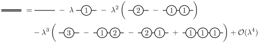
Figure 1: Diagrammatic representation of the NC retarded/advanced Green’s operator (double line) in terms of the commutative retarded/advanced Green’s operator (single line) and the NC corrections to the equation of motion $P_{(n)}$ (vertices labeled by $n$).

6 Examples II: Deformed Green’s functions

In this section we derive the leading NC corrections to the Green’s operators of the NC Klein–Gordon operators studied in Section 4. For the deformed Randall–Sundrum spacetime, the derivation of the Green’s functions from (4.11) is straightforward, see (4.12) for a particular choice of deformation. We study the remaining examples in this section. The focus is on the illustration of the formalism, but the results of this section can also be useful for phenomenological studies of (quantum) field theories on curved NC spacetimes, e.g. for NC cosmology or black hole physics.

6.1 Deformed Minkowski spacetime

We start with the simplest nontrivial example given by the equation of motion operator (4.3) on the $\kappa$-type deformed Minkowski spacetime. Even though this equation of motion operator can be diagonalized using plane waves, we use the perturbative expansion (see Fig. 1) in order to illustrate the formalism.

The leading NC corrections of the equation of motion operator (4.3) are given by

$$P_{(1)}=\frac{3i}{2}\partial_{t}\left(\partial_{t}^{2}-\triangle+m^{2}\right)=-\frac{3i}{2}\partial_{t}\circ P_{(0)},$$

$$P_{(2)}=-\frac{9}{4}\partial_{t}^{2}\circ P_{(0)}-2~{}\partial_{t}^{2}\circ\triangle.$$

Note that the order $\lambda^{1}$ correction is imaginary. This does not violate the reality of our field theory since the equation of motion operator resulting from the action $\tilde{P}_{\star}[\Phi]=P_{\star}[\Phi]\star\mathrm{vol}_{\star}$ is indeed real, but regarded as a top-form. It has been shown in [32] how to construct the space of real solutions of such deformed wave operators.

We calculate the corrections to the Green’s operators using Fig. 1, and find

$$\Delta_{(1)\pm}=-\Delta_{\pm}\circ P_{(1)}\circ\Delta_{\pm}=\frac{3i}{2}\Delta_{\pm}\circ\partial_{t}\circ P_{(0)}\circ\Delta_{\pm}=\frac{3i}{2}\Delta_{\pm}\circ\partial_{t},$$ (6.1a)

$$\Delta_{(2)\pm}=2\Delta_{\pm}\circ\partial_{t}^{2}\circ\triangle\circ\Delta_{\pm},$$ (6.1b)

where we have used $P_{(0)}\circ\Delta_{\pm}=\text{id}$, which results from the very definition of the Green’s operator.

Next, we extract the NC Green’s functions $\tilde{\Delta}_{\star\pm}(x,y)$, i.e. the integral kernels of the operators $\Delta_{\star\pm}$ defined by

$$\Delta_{\star\pm}[\varphi](x)=:\int\tilde{\Delta}_{\star\pm}(x,y)\varphi(y)\mathrm{vol}_{y},$$

for all functions $\varphi$ of compact support. Using (6.1) and integration by parts we find

$$\tilde{\Delta}_{\star\pm}(x,y)=\tilde{\Delta}_{\pm}(x,y)-\frac{3i\lambda}{2}\partial_{t_{y}}\tilde{\Delta}_{\pm}(x,y)+2\lambda^{2}\!\int\!\tilde{\Delta}_{\pm}(x,z)\partial_{t_{z}}^{2}\triangle_{z}\tilde{\Delta}_{\pm}(z,y)d^{4}z+\mathcal{O}(\lambda^{3}).\!\!$$ (6.2)

The integral in the order-$\lambda^{2}$ part, $\tilde{\Delta}_{(2)\pm}$, can be evaluated explicitly using the momentum space representation of the classical Green’s functions. It turns out that this integral does not require an infrared regularization and we obtain

$$\tilde{\Delta}_{(2)\pm}(x,y)=\mp\Theta\left(\pm t_{z}\right)\int\frac{d^{3}p}{(2\pi)^{3}}e^{-i\mathbf{p}\mathbf{z}}\mathbf{p}^{2}\left(t_{z}\cos(E_{p}t_{z})+\frac{\sin(E_{p}t_{z})}{E_{p}}\right),$$

where $E_{p}=\sqrt{\mathbf{p}^{2}+m^{2}}$, $t_{z}=t_{x}-t_{y}$, $\mathbf{z}=\mathbf{x}-\mathbf{y}$ and $\Theta$ is the Heaviside step-function. For a massless field the remaining Fourier transformation is easily performed and one finds that the support of the correction $\tilde{\Delta}_{(2)\pm}$ is, as expected, on the forward/backward lightcone. Since the explicit formula is not very instructive we do not include it here.

Note that the deformed Green’s functions $\tilde{\Delta}_{\star\pm}(x,y)$ are not real. This can be understood from the fact that the scalar-valued wave operator is not real, thus leading to complex Green’s functions. The sources to be considered physical are those leading to real solutions of the inhomogeneous problem $P_{\star}[\psi]=\varphi$. Multiplying both sides with the volume form $\mathrm{vol}_{\star}$ from the right we find $\tilde{P}_{\star}[\psi]=P_{\star}[\psi]\star\mathrm{vol}_{\star}=\varphi\star\mathrm{vol}_{\star}$. Thus, the physical sources $\varphi$ have to obey the top-form reality condition $(\varphi\star\mathrm{vol}_{\star})^{\ast}=\varphi\star\mathrm{vol}_{\star}$, which in general implies $\varphi^{\ast}\neq\varphi$ if the volume form is not central.

Applying the Green’s operators to physical sources we find no nontrivial corrections at order $\lambda^{1}$. This is because a physical source $\varphi=\sum\lambda^{n}\varphi_{(n)}$ has to fulfil $(\varphi\star\mathrm{vol}_{\star})^{\ast}=\varphi\star\mathrm{vol}_{\star}$, which implies in our particular model $\varphi_{(0)}^{\ast}=\varphi_{(0)}$ and $\mathfrak{Im}(\varphi_{(1)})=-\frac{3}{2}\partial_{t}\varphi_{(0)}$. Thus, we obtain

$$\Delta_{\star\pm}[\varphi]=\Delta_{\pm}\left[\varphi_{(0)}+\lambda\varphi_{(1)}+\frac{3i\lambda}{2}\partial_{t}\varphi_{(0)}\right]+\mathcal{O}(\lambda^{2})=\Delta_{\pm}[\varphi_{(0)}+\lambda\mathfrak{Re}(\varphi_{(1)})]+\mathcal{O}(\lambda^{2}).$$

6.2 Deformed FRW spacetime

We derive the second-order corrections to the Green’s operators for the NC de Sitter universes discussed in Section 4.2. Since the wave operators of both models are quite similar in their structure, see (4.5) and (4.6), we derive the corrections for the first model and can obtain the corrections for the second model by replacing $\mathcal{D}\to-H\partial_{\phi}$. Similar to the Minkowski model discussed before, the first nontrivial NC correction to the Green’s operators acting on physical sources is of order $\lambda^{2}$. The leading NC corrections of the wave operator (4.5) read

$$P_{(1)}=-\frac{3i}{2}\mathcal{D}\circ P_{(0)},\qquad P_{(2)}=-\frac{9}{4}\mathcal{D}^{2}\circ P_{(0)}-2\mathcal{D}^{2}\circ\left(e^{-2Ht}\triangle\right).$$

Via Fig. 1 this leads to the following NC corrections to the Green’s operators

$$\Delta_{(1)\pm}=\frac{3i}{2}\,\Delta_{\pm}\circ\mathcal{D},\qquad\Delta_{(2)\pm}=2\Delta_{\pm}\circ\mathcal{D}^{2}\circ\left(e^{-2Ht}\triangle\right)\circ\Delta_{\pm}.$$

The NC integral kernel $\tilde{\Delta}_{\star\pm}(x,y)$ can be obtained by integration by parts and reads

$$\tilde{\Delta}_{\star\pm}(x,y)=\tilde{\Delta}_{\pm}(x,y)-\frac{3i\lambda}{2}\mathcal{D}_{y}\tilde{\Delta}_{\pm}(x,y)$$

$$\phantom{\tilde{\Delta}_{\star\pm}(x,y)=}{}+2\lambda^{2}\int\tilde{\Delta}_{\pm}(x,z)\mathcal{D}^{2}_{z}\,e^{-2Ht_{z}}\triangle_{z}\tilde{\Delta}_{\pm}(z,y)\mathrm{vol}_{z}+\mathcal{O}(\lambda^{3}).$$

This shows that the corrections have a similar structure to the Minkowski case (6.2). The explicit evaluation of the integral in the order-$\lambda^{2}$ part and the investigation of its IR regulator (in)dependence is beyond the scope of this work.

6.3 Deformed Schwarzschild black hole

We derive for completeness the second-order corrections to the Green’s operators for the NC Schwarzschild spacetime discussed in Section 4.3. The leading NC corrections of the equation of motion operator (4.7) read

$$P_{(1)}=-\frac{3i}{2}\,\partial_{t}\circ P_{(0)},$$

$$P_{(2)}=-\frac{9}{4}\partial_{t}^{2}\circ P_{(0)}-2\partial_{t}^{2}\circ\triangle_{\mathrm{bh}}+\mathfrak{B}_{1}+\mathfrak{B}_{2}=:-\frac{9}{4}\partial_{t}^{2}\circ P_{(0)}+\widehat{P}_{(2)},$$

where the spatial Laplacian $\triangle_{\mathrm{bh}}$ and the differential operators $\mathfrak{B}_{1}$ and $\mathfrak{B}_{2}$ are defined by

$$\triangle_{\mathrm{bh}}[\varphi]:=\frac{1}{r^{2}}\partial_{r}\left(r^{2}Q(r)\partial_{r}\varphi\right)+\frac{1}{r^{2}}\triangle_{S^{2}}\varphi,$$

$$\mathfrak{B}_{1}[\varphi]:=\frac{1}{8Q(r)^{3}}\frac{r_{s}}{r}\left(7-5\frac{r_{s}}{r}\right)\partial_{t}^{4}\varphi,$$

$$\mathfrak{B}_{2}[\varphi]:=\frac{11r_{s}}{8r^{2}}\partial_{r}\left(r\partial_{r}\partial_{t}^{2}\varphi\right).$$

Via Fig. 1 this leads to the following NC corrections to the Green’s operators

$$\Delta_{(1)\pm}=\frac{3i}{2}\,\Delta_{\pm}\circ\partial_{t},$$

$$\Delta_{(2)\pm}=\Delta_{\pm}\circ\left(2\partial_{t}^{2}\circ\triangle_{\mathrm{bh}}-\mathfrak{B}_{1}-\mathfrak{B}_{2}\right)\circ\Delta_{\pm}=-\Delta_{\pm}\circ\widehat{P}_{(2)}\circ\Delta_{\pm}.$$

The NC integral kernel $\tilde{\Delta}_{\star\pm}(x,y)$ can be obtained by integration by parts and reads

$$\tilde{\Delta}_{\star\pm}(x,y)=\tilde{\Delta}_{\pm}(x,y)-\frac{3i\lambda}{2}\partial_{t_{y}}\tilde{\Delta}_{\pm}(x,y)-\lambda^{2}\int\tilde{\Delta}_{\pm}(x,z)\widehat{P}_{(2)z}\tilde{\Delta}_{\pm}(z,y)\mathrm{vol}_{z}+\mathcal{O}(\lambda^{3}).$$

Again, we do not evaluate the integral in the order-$\lambda^{2}$ part explicitly. The calculation might be simplified drastically if one considers a two-dimensional reduction of the black hole by only taking into account the isotropic modes (with spherical harmonic $Y_{00}(\zeta,\phi)$).

7 Conclusions and outlook

In this article we have investigated classical scalar field theories on curved NC spacetimes, with the NC deformations given by a large class of Drinfel’d twists. Our models in particular include position dependent NC. We have shown how to construct a deformed action for a real scalar field and how to derive the corresponding equation of motion in both, a geometric (global) and a coordinate-based (local) approach. Subsequently, we have provided explicit examples of deformed Klein–Gordon operators on NC Minkowski, de Sitter, Schwarzschild and Randall–Sundrum spacetimes. Our deformed background spacetimes are chosen such that the NC Einstein equations of Wess et al. [7, 8] are solved exactly. We have then discussed the construction of the deformed Green’s operators corresponding to the deformed wave operators and provided a diagrammatic formalism for their perturbative calculation. The formalism has been applied to field theory on NC Minkowski, de Sitter and Schwarzschild spacetimes in order to study the second-order correction to the advanced and retarded Green’s functions.

This work is restricted to the level of classical field theory, since the construction of physical quantum states in the formalism [32] has not been achieved yet. Nevertheless, the perturbative construction of Green’s functions discussed in the present paper can be used to construct the algebras of the corresponding QFT, since the canonical commutation relations are determined by the Green’s functions [32]. Once the construction of quantum states in our NC QFT is understood, the results obtained here can be applied in order to study NC effects in primordial power-spectra of scalar fields and NC effects in the vicinity of Schwarzschild black holes. For the construction of quantum states the approach of [42] might prove to be helpful.

References

- [1]
- [2] Connes A., Noncommutative geometry, Academic Press, Inc., San Diego, CA, 1994.
- [3] Landi G., An introduction to noncommutative spaces and their geometry, hep-th/9701078.
-
[4]
Doplicher S., Fredenhagen K., Roberts J.E.,
Spacetime quantization induced by classical gravity,
Phys. Lett. B 331 (1994), 39–44.
Doplicher S., Fredenhagen K., Roberts J.E., The quantum structure of spacetime at the Planck scale and quantum fields, Comm. Math. Phys. 172 (1995), 187–220, hep-th/0303037. - [5] Seiberg N., Witten E., String theory and noncommutative geometry, J. High Energy Phys. 1999 (1999), no. 9, 032, 93 pages, hep-th/9908142.
-
[6]
Amelino-Camelia G., Smolin L., Starodubtsev A.,
Quantum symmetry, the cosmological constant and Planck-scale phenomenology,
Classical Quantum Gravity 21 (2004), 3095–3110,
hep-th/0306134.
Freidel L., Kowalski-Glikman J., Smolin L., 2+1 gravity and doubly special relativity, Phys. Rev. D 69 (2004), 044001, 7 pages, hep-th/0307085. - [7] Aschieri P., Blohmann C., Dimitrijević M., Meyer F., Schupp P., Wess J., A gravity theory on noncommutative spaces, Classical Quantum Gravity 22 (2005), 3511–3532, hep-th/0504183.
- [8] Aschieri P., Dimitrijević M., Meyer F., Wess J., Noncommutative geometry and gravity, Classical Quantum Gravity 23 (2006), 1883–1911, hep-th/0510059.
- [9] Kürkçüoǧlu S., Sämann C., Drinfeld twist and general relativity with fuzzy spaces, Classical Quantum Gravity 24 (2007), 291–311, hep-th/0606197.
- [10] Chamseddine A.H., Felder G., Fröhlich J., Gravity in noncommutative geometry, Comm. Math. Phys. 155 (1993), 205–217, hep-th/9209044.
- [11] Chamseddine A.H., Complexified gravity in noncommutative spaces, Comm. Math. Phys. 218 (2001), 283–292, hep-th/0005222.
- [12] Chamseddine A.H., Deforming Einstein’s gravity, Phys. Lett. B 504 (2001), 33–37, hep-th/0009153.
- [13] Cardella M.A., Zanon D., Noncommutative deformation of four-dimensional Einstein gravity, Classical Quantum Gravity 20 (2003), L95–L103, hep-th/0212071.
- [14] Chamseddine A.H., gravity with complex vierbein and its noncommutative extension, Phys. Rev. D 69 (2004), 024015, 8 pages, hep-th/0309166.
- [15] Banerjee R., Mukherjee P., Samanta S., Lie algebraic noncommutative gravity, Phys. Rev. D 75 (2007), 125020, 7 pages, hep-th/0703128.
-
[16]
Aschieri P., Castellani L.,
Noncommutative gravity coupled to fermions,
J. High Energy Phys. 2009 (2009), no. 6, 086, 18 pages,
arXiv:0902.3817.
Aschieri P., Castellani L., Noncommutative supergravity in and , J. High Energy Phys. 2009 (2009), no. 6, 087, 22 pages, arXiv:0902.3823. -
[17]
Madore J., Mourad J.,
Quantum space-time and classical gravity,
J. Math. Phys. 39 (1998), 423–442,
gr-qc/9607060.
Madore J., An introduction to noncommutative differential geometry and its physical applications, 2nd ed., London Mathematical Society Lecture Note Series, Vol. 257, Cambridge University Press, Cambridge, 1999.
Langmann E., Szabo R.J., Teleparallel gravity and dimensional reductions of noncommutative gauge theory, Phys. Rev. D 64 (2001), 104019, 15 pages, hep-th/0105094.
Chamseddine A.H., An invariant action for noncommutative gravity in four dimensions, J. Math. Phys. 44 (2003), 2534–2541, hep-th/0202137.
García-Compeán H., Obregón O., Ramírez C., Sabido M., Noncommutative self-dual gravity, Phys. Rev. D 68 (2003), 044015, 8 pages, hep-th/0302180.
Vassilevich D.V., Quantum noncommutative gravity in two dimensions, Nuclear Phys. B 715 (2005), 695–712, hep-th/0406163.
Calmet X., Kobakhidze A., Noncommutative general relativity, Phys. Rev. D 72 (2005), 045010, 5 pages, hep-th/0506157.
Burić M., Grammatikopoulos T., Madore J., Zoupanos G., Gravity and the structure of noncommutative algebras, J. High Energy Phys. 2006 (2006), no. 4, 054, 16 pages, hep-th/0603044.
Majid S., Algebraic approach to quantum gravity. II. Noncommutative spacetime, hep-th/0604130.
Majid S., Algebraic approach to quantum gravity. III. Noncommmutative Riemannian geometry, hep-th/0604132.
Szabo R.J., Symmetry, gravity and noncommutativity, Classical Quantum Gravity 23 (2006), R199–R242, hep-th/0606233.
Balachandran A.P., Pinzul A., Qureshi B.A., Vaidya S., Twisted gauge and gravity theories on the Groenewold–Moyal plane, Phys. Rev. D 76 (2007), 105025, 10 pages, arXiv:0708.0069.
Müller-Hoissen F., Noncommutative geometries and gravity, in Recent Developments in Gravitation and Cosmology, AIP Conf. Proc., Vol. 977, Amer. Inst. Phys., Melville, NY, 2008, 12–29, arXiv:0710.4418.
Vassilevich D.V., Diffeomorphism covariant star products and noncommutative gravity, Classical Quantum Gravity 26 (2009), 145010, 8 pages, arXiv:0904.3079.
Vassilevich D.V., Tensor calculus on noncommutative spaces, Classical Quantum Gravity 27 (2010), 095020, 16 pages, arXiv:1001.0766. - [18] Rivelles V.O., Noncommutative field theories and gravity, Phys. Lett. B 558 (2003), 191–196, hep-th/0212262.
-
[19]
Yang H.S.,
Emergent gravity from noncommutative space-time,
Internat. J. Modern Phys. A 24 (2009), 4473–4517,
hep-th/0611174.
Yang H.S., On the correspondence between noncommuative field theory and gravity, Modern Phys. Lett. A 22 (2007), 1119–1132, hep-th/0612231. -
[20]
Steinacker H.,
Emergent gravity from noncommutative gauge theory,
J. High Energy Phys. 2007 (2007), no. 12, 049, 36 pages,
arXiv:0708.2426.
Steinacker H., Emergent gravity and noncommutative branes from Yang–Mills matrix models, Nuclear Phys. B 810 (2009), 1–39, arXiv:0806.2032. - [21] Dito G., Sternheimer D., Deformation quantization: genesis, developments and metamorphoses, in Deformation Quantization (Strasbourg, 2001), IRMA Lect. Math. Theor. Phys., Vol. 1, de Gruyter, Berlin, 2002, 9–54, math.QA/0201168.
- [22] Drinfel’d V.G., On constant quasiclassical solutions of the Yang–Baxter equations, Soviet Math. Dokl. 28 (1983), 667–671.
- [23] Ohl T., Schenkel A., Symmetry reduction in twisted noncommutative gravity with applications to cosmology and black holes, J. High Energy Phys. 2009 (2009), no. 1, 084, 22 pages, arXiv:0810.4885.
- [24] Schupp P., Solodukhin S., Exact black hole solutions in noncommutative gravity, arXiv:0906.2724.
- [25] Ohl T., Schenkel A., Cosmological and black hole spacetimes in twisted noncommutative gravity, J. High Energy Phys. 2009 (2009), no. 10, 052, 12 pages, arXiv:0906.2730.
- [26] Aschieri P, Castellani L., Noncommutative gravity solutions, J. Geom. Phys. 60 (2010), 375–393, arXiv:0906.2774.
- [27] Asakawa T., Kobayashi S., Noncommutative solitons of gravity, Classical Quantum Gravity 27 (2010), 105014, 20 pages, arXiv:0911.2136.
- [28] Stern A., Emergent Abelian gauge fields from noncommutative gravity, SIGMA 6 (2010), 019, 15 pages, arXiv:0912.3021.
-
[29]
Chu C.S., Greene B.R., Shiu G.,
Remarks on inflation and noncommutative geometry,
Modern Phys. Lett. A 16 (2001), 2231–2240,
hep-th/0011241.
Lizzi F., Mangano G., Miele G., Peloso M., Cosmological perturbations and short distance physics from noncommutative geometry, J. High Energy Phys. 2002 (2002), no. 6, 049, 16 pages, hep-th/0203099.
Brandenberger R., Ho P.-M., Noncommutative spacetime, stringy spacetime uncertainty principle, and density fluctuations, Phys. Rev. D 66 (2002), 023517, 10 pages, hep-th/0203119.
Huang Q.-G., Li M., CMB power spectrum from noncommutative spacetime, J. High Energy Phys. 2003 (2003), no. 6, 014, 7 pages, hep-th/0304203.
Huang Q.G., Li M., Noncommutative inflation and the CMB multipoles, J. Cosmol. Astropart. Phys. 0311 (2003), 001, 9 pages, astro-ph/0308458.
Tsujikawa S., Maartens R., Brandenberger R., Non-commutative inflation and the CMB, Phys. Lett. B 574 (2003), 141–148, astro-ph/0308169.
Kim H.-C., Yee J.H., Rim C., Density fluctuations in kappa-deformed inflationary universe, Phys. Rev. D 72 (2005), 103523, 13 pages, gr-qc/0506122.
Fatollahi A.H., Hajirahimi M., Noncommutative black-body radiation: implications on cosmic microwave background, Europhys. Lett. 75 (2006), 542–547, astro-ph/0607257.
Akofor E., Balachandran A.P., Jo S.G., Joseph A., Qureshi B.A., Direction-dependent CMB power spectrum and statistical anisotropy from noncommutative geometry, J. High Energy Phys. 2008 (2008), no. 5, 092, 21 pages, arXiv:0710.5897.
Akofor E., Balachandran A.P., Joseph A., Pekowsky L., Qureshi B.A., Constraints from CMB on spacetime noncommutativity and causality violation, Phys. Rev. D 79 (2009), 063004, 5 pages, arXiv:0806.2458.
Fabi S., Harms B., Stern A., Noncommutative corrections to the Robertson–Walker metric, Phys. Rev. D 78 (2008), 065037, 7 pages, arXiv:0808.0943. -
[30]
Dolan B.P., Gupta K.S., Stern A.,
Noncommutative BTZ black hole and discrete time,
Classical Quantum Gravity 24 (2007), 1647–1655,
hep-th/0611233.
Chaichian M., Tureanu A., Zet G., Corrections to Schwarzschild solution in noncommutative gauge theory of gravity, Phys. Lett. B 660 (2008), 573–578, arXiv:0710.2075.
Mukherjee P., Saha A., Reissner–Nordstrom solutions in noncommutative gravity, Phys. Rev. D 77 (2008), 064014, 7 pages, arXiv:0710.5847.
Burić M., Madore J., Spherically symmetric non-commutative space: , Eur. Phys. J. C 58 (2008), 347–353, arXiv:0807.0960.
Nicolini P., Noncommutative black holes, the final appeal to quantum gravity: a review, Internat. J. Modern Phys. A 24 (2009), 1229–1308, arXiv:0807.1939.
Wang D., Zhang R.B., Zhang X., Quantum deformations of Schwarzschild and Schwarzschild–de Sitter spacetimes, Classical Quantum Gravity 26 (2009), 085014, 14 pages, arXiv:0809.0614.
Di Grezia E., Esposito G., Non-commutative Kerr black hole, arXiv:0906.2303.
Banerjee R., Chakraborty B., Ghosh S., Mukherjee P., Samanta S., Topics in noncommutative geometry inspired physics, Found. Phys. 39 (2009), 1297–1345, arXiv:0909.1000. -
[31]
Oeckl R.,
Untwisting noncommutative and the equivalence of quantum field theories,
Nuclear Phys. B 581 (2000), 559–574,
hep-th/0003018.
Bahns D., Doplicher S., Fredenhagen K., Piacitelli G., Ultraviolet finite quantum field theory on quantum spacetime, Comm. Math. Phys. 237 (2003), 221–241, hep-th/0301100.
Chaichian M., Mnatsakanova M.N., Nishijima K., Tureanu A., Vernov Yu.S., Towards an axiomatic formulation of noncommutative quantum field theory, hep-th/0402212.
Paschke M., Verch R., Local covariant quantum field theory over spectral geometries, Classical Quantum Gravity 21 (2004), 5299–5316, gr-qc/0405057.
Zahn J., Remarks on twisted noncommutative quantum field theory, Phys. Rev. D 73 (2006), 105005, 6 pages, hep-th/0603231.
Bu J.-G., Kim H.-C., Lee Y., Vac C.H., Yee J.H., Noncommutative field theory from twisted Fock space, Phys. Rev. D 73 (2006), 125001, 10 pages, hep-th/0603251.
Gayral V., Jureit J.H., Krajewski T., Wulkenhaar R., Quantum field theory on projective modules, hep-th/0612048.
Fiore G., Wess J., Full twisted Poincaré symmetry and quantum field theory on Moyal–Weyl spaces, Phys. Rev. D 75 (2007), 105022, 13 pages, hep-th/0701078.
Freidel L., Kowalski-Glikman J., Nowak S., Field theory on -Minkowski space revisited: Noether charges and breaking of Lorentz symmetry, Internat. J. Modern Phys. A 23 (2008), 2687–2718, arXiv:0706.3658.
Grosse H., Lechner G., Wedge-local quantum fields and noncommutative Minkowski space, J. High Energy Phys. 2007 (2007), no. 11, 012, 26 pages, arXiv:0706.3992.
Arzano M., Marciano A., Fock space, quantum fields and kappa-Poincaré symmetries, Phys. Rev. D 76 (2007), 125005, 14 pages, arXiv:0707.1329.
Daszkiewicz M., Lukierski J., Woronowicz M., Towards quantum noncommutative -deformed field theory, Phys. Rev. D 77 (2008), 105007, 10 pages, arXiv:0708.1561.
Balachandran A.P., Pinzul A., Qureshi B.A., Twisted Poincaré invariant quantum field theories, Phys. Rev. D 77 (2008), 025021, 9 pages, arXiv:0708.1779.
Aschieri P., Lizzi F., Vitale P., Twisting all the way: from classical mechanics to quantum fields, Phys. Rev. D 77 (2008), 025037, 16 pages, arXiv:0708.3002.
Arzano M., Quantum fields, non-locality and quantum group symmetries, Phys. Rev. D 77 (2008), 025013, 5 pages, arXiv:0710.1083.
Daszkiewicz M., Lukierski J., Woronowicz M., -deformed oscillators, the choice of star product and free -deformed quantum fields, J. Phys. A: Math. Theor. 42 (2009), 355201, 18 pages, arXiv:0807.1992.
Grosse H., Lechner G., Noncommutative deformations of Wightman quantum field theories, J. High Energy Phys. 2008 (2008), no. 9, 131, 29 pages, arXiv:0808.3459.
Fiore G., On second quantization on noncommutative spaces with twisted symmetries, J. Phys. A: Math. Theor. 43 (2010), 155401, 39 pages, arXiv:0811.0773.
Borris M., Verch R., Dirac field on Moyal–Minkowski spacetime and non-commutative potential scattering, Comm. Math. Phys. 293 (2010), 399–448, arXiv:0812.0786.
Aschieri P., Star product geometries, Russ. J. Math. Phys. 16 (2009), 371–383, arXiv:0903.2457. - [32] Ohl T., Schenkel A., Algebraic approach to quantum field theory on a class of noncommutative curved spacetimes, arXiv:0912.2252.
- [33] Wald R.M., Quantum field theory in curved spacetime and black hole thermodynamics, Chicago Lectures in Physics, University of Chicago Press, Chicago, IL, 1994.
- [34] Bär C., Ginoux N., Pfäffle F., Wave equations on Lorentzian manifolds and quantization, ESI Lectures in Mathematics and Physics, European Mathematical Society (EMS), Zürich, 2007, arXiv:0806.1036.
- [35] Reshetikhin N., Multiparameter quantum groups and twisted quasitriangular Hopf algebras, Lett. Math. Phys. 20 (1990), 331–335.
- [36] Jambor C., Sykora A., Realization of algebras with the help of -products, hep-th/0405268.
-
[37]
Bu J.-G., Kim H.-C., Lee Y., Vac C.H., Yee J.H.,
-deformed spacetime from twist,
Phys. Lett. B 665 (2008), 95–99,
hep-th/0611175.
Borowiec A., Pachol A., -Minkowski spacetime as the result of Jordanian twist deformation, Phys. Rev. D 79 (2009), 045012, 11 pages, arXiv:0812.0576. -
[38]
Dimakis A., Madore J.,
Differential calculi and linear connections,
J. Math. Phys. 37 (1996), 4647–4661,
q-alg/9601023.
Cerchiai L., Fiore G., Madore J., Frame formalism for the -dimensional quantum Euclidean spaces, Internat. J. Modern Phys. B 14 (2000), 2305–2314, math.QA/0007044. - [39] Ohl T., Schenkel A., Uhlemann C.F., Spacetime noncommutativity in models with warped extradimensions, J. High Energy Phys. 2010 (2010), no. 7, 029, 16 pages, arXiv:1002.2884.
- [40] Schenkel A., Uhlemann C.F., High energy improved scalar quantum field theory from noncommutative geometry without UV/IR-mixing, arXiv:1002.4191.
- [41] Hořava P., Quantum gravity at a Lifshitz point, Phys. Rev. D 79 (2009), 084008, 15 pages, arXiv:0901.3775.
-
[42]
Dappiaggi C., Moretti V., Pinamonti N.,
Cosmological horizons and reconstruction of quantum field theories,
Comm. Math. Phys. 285 (2009), 1129–1163,
arXiv:0712.1770.
Dappiaggi C., Moretti V., Pinamonti N., Distinguished quantum states in a class of cosmological spacetimes and their Hadamard property, J. Math. Phys. 50 (2009), 062304, 38 pages, arXiv:0812.4033.
Dappiaggi C., Moretti V., Pinamonti N., Rigorous construction and Hadamard property of the Unruh state in Schwarzschild spacetime, arXiv:0907.1034.