Generalized Khinchin Theorem for a Class of Aging Processes

Abstract

The Khinchin theorem provides the condition that a stationary process is ergodic, in terms of the behavior of the corresponding correlation function. Many physical systems are governed by non-stationary processes in which correlation functions exhibit aging. We classify the ergodic behavior of such systems and provide a generalization of Khinchin’s theorem. Our work quantifies deviations from ergodicity in terms of aging correlation functions. Using the framework of the fractional Fokker-Planck equation we obtain a simple analytical expression for the two-time correlation function of the particle displacement in a general binding potential, revealing universality in the sense that the binding potential only enters into the prefactor through the first two moments of the corresponding Boltzmann distribution. We discuss applications to experimental data from systems exhibiting anomalous dynamics.

The dynamics of physical observables is commonly quantified in terms of time dependent correlation functions; these are pair products of dynamic observables $O(t_{1})$ and $O(t_{2})$, that are averaged over an ensemble, $C(t_{2},t_{1})=\langle O(t_{2})O(t_{1})\rangle$. When such a correlation function describes a stationary process, $C(t_{2},t_{1})$ is a function of the time difference only, that is, $C(t_{2},t_{1})=C(|t_{2}-t_{1}|)$. For such processes the correlation function contains the dynamical information on other physical observables via fundamental theorems [1]. For instance, the Wiener-Khinchin theorem relates the power spectrum to the correlation function; or the fluctuation-dissipation theorem connects correlation functions to linear response functions. Another well known example is Khinchin’s theorem [2], that provides a criterion for ergodicity of a process in terms of the corresponding stationary correlation function. However, the stationarity property is found to be violated in numerous systems (see below). These systems exhibit aging properties, that are intimately connected to the non-stationary behavior. Correlation functions in aging systems behave very differently from their stationary counterparts [3, 4, 5, 6]. For instance, such non-stationary systems may be characterized by correlation functions of the type $C(t_{2},t_{1})=h(t_{1}/t_{2})$ (if $t_{2}\geq t_{1}$), i.e., the two times enter as a quotient rather than their difference. This non-stationary behavior is also connected to a breaking of ergodicity in the sense that long time averages differ from ensemble averages of the same quantities [3, 7, 8, 9, 10]. The relation between correlation functions and ergodicity breaking can be quantified by the Edwards-Anderson parameter [3], see below.

We here present a generalization of the Khinchin theorem for aging systems, relating fluctuations of time averages to the corresponding aging correlation function, that we calculate for a class of important stochastic processes. In particular we derive an analytical expression for the two-time position correlation function in the presence of an external binding potential $U(x)$ based on the the general framework of the fractional Fokker-Planck equation [11, 12, 13]. The latter describes systems in which the mean squared displacement in free space scales as $\langle x^{2}(t)\rangle\propto t^{\alpha}$, where the anomalous diffusion exponent $\alpha$ ranges in the interval $0<\alpha<1$ [12, 13, 14]. Our results for the correlation function are quite general and could also be applied to continuous time random walk (CTRW) systems in confined geometries and mean field descriptions of models such as the quenched trap model [14]. In particular, we show that for sufficiently long times the correlation function behaves universally, and the dependence on the potential $U(x)$ enters only in the prefactor through the first two moments of the corresponding Boltzmann distribution. We also discuss aging properties of the correlation function and the time averaged mean squared displacement. Moreover we demonstrate agreement of our results with experimental data.

Physical systems displaying non-stationary behavior like aging and ergodicity breaking traditionally included glassy systems such as spin glasses [3], colloidal glasses [15], gels [16], turbulent systems [17], or tracer dispersion in subsurface hydrology [18], among others. More recently advanced single-molecule experiments reveal other types of complex systems with similar behavior. These are systems exhibiting anomalous diffusion and slow, non-exponential relaxation dynamics [14, 12, 13, 19]. For instance, they include blinking quantum dots [20, 21, 22, 23], or biologically relevant systems. The latter include subdiffusion of tracer particles in living biological cells [24, 25, 26, 27, 28, 29] or reconstituted crowding systems [30, 31, 32, 33], protein conformational dynamics [34], or the motion of bacteria in a biofilm [35]. Here we show how the knowledge of the aging correlation function allows us to quantify the non-ergodic behavior of the process.

0.1 Correlation functions and ergodicity

The concept of ergodicity plays a central role in statistical physics. Boltzmann’s ergodic hypothesis relates the time average of a physical observable $O$ to its ensemble average and states that both are equal in the long time limit:

$$\overline{O}\equiv\lim_{t\to\infty}\frac{1}{t}\int_{0}^{t}O(t^{\prime})dt^{\prime}=\langle O\rangle.$$ (1)

where $\langle\cdot\rangle$ represent an ensemble average with respect to a steady state probability distribution. The connection between the ergodic hypothesis and correlation functions was established by Khinchin [2], a work of considerable impact to statistical physics [36]. Khinchin’s theorem states that an observable $O(t)$ is ergodic if the associated correlation function is “irreversible”, in the sense that if $O(t)$ fulfills

$$\lim_{\Delta\to\infty}\langle O(t_{1}+\Delta)O(t_{1})\rangle=\langle O\rangle^{2}\qquad\left(\Delta=|t_{2}-t_{1}|\right),$$ (2)

then Eq. (1) holds. In the derivation of Khinchin’s theorem it is assumed that the process is stationary and the system reached a steady state, $C(t_{2},t_{1})=\langle O(t_{2})O(t_{1})\rangle=C(\Delta)$. Thus the irreversibility condition corresponds to the requirement $C(\Delta)=\langle O\rangle^{2}$ for $\Delta\to\infty$. Note that for stationary systems [37] irreversibility is a broader concept than the ergodic hypothesis, and that therefore Khinchin’s theorem cannot always be reversed. The case of power-law decaying correlation functions was treated previously based on the generalized Langevin equation [38, 39]. This gives rise to a stationary process, such that Khinchin’s theorem holds for this kind of anomalous dynamics.

Having in mind the aforementioned non-stationary systems, the following question arises: Does irreversibility imply ergodicity also for aging systems? And if not, what theorem replaces Khinchin’s? To answer these questions we quantify ergodicity in terms of second moments, namely if $\left<\overline{O}^{2}\right>=\langle O\rangle^{2}$ the dynamics is ergodic, as originally pointed out by Khinchin and $\left<\overline{O}\right>=\langle O\rangle$ always holds for processes where $\langle O(t)\rangle$ is constant for long enough time. From Eq. (1) we find for the second moment

$$\left<\overline{O(t)}^{2}\right>=\frac{1}{t^{2}}\int_{0}^{t}\int_{0}^{t}\langle O(t_{2})O(t_{1})\rangle\,dt_{2}\,dt_{1}.$$ (3)

Assuming aging behavior for the correlation function in the above form $\langle O(t_{2})O(t_{1})\rangle=h(t_{1}/t_{2})$ ($t_{2}\geq t_{1}$) (i.e., we use the aging regime as the “steady state” of the system similarly to invoking stationarity in Khinchin’s theorem) Eq. (3) becomes

$$\left<\overline{O(t)}^{2}\right>=\frac{2}{t^{2}}\int_{0}^{t}\int_{0}^{t_{2}}h(t_{1}/t_{2})dt_{1}dt_{2}.$$ (4)

After the substitution $t_{1}^{2}+t_{2}^{2}=r^{2}$ and $t_{1}/t_{2}=\tan(\theta)$ we find

$$\left<\overline{O}^{2}\right>=\int_{0}^{1}h(z)\,dz.$$ (5)

This is a general relation between the fluctuation of the time averaged and ensemble averaged correlation functions. For ergodicity to hold, we consequently require that in the long time limit the condition

$$\left<O\right>^{2}=\int_{0}^{1}h(z)\,dz$$ (6)

is fulfilled. Simultaneously we can rewrite the irreversibility condition $\lim_{\Delta\to\infty}h(t\big{/}t+\Delta)=\left<O\right>^{2}$ in the form

$$\lim_{z\to 0}h(z)=\left<O\right>^{2}.$$ (7)

Thus, to fulfill Eq. (6) the condition (7) is not sufficient, and Khinchin’s theorem does not hold for aging systems. Namely irreversibility does not imply ergodicity in aging system. We define a generalization of Khinchin’s theorem stating that in the case of irreversible dynamics the condition for ergodicity in an aging system is given by

$$\lim_{z\to 0}h(z)=\int_{0}^{1}h(z)\,dz.$$ (8)

The knowledge of the correlation function resolves the question of ergodicity for a system. More importantly, by help of Eq. (5) the correlation function allows one to quantify the fluctuations of the time averages and ergodicity breaking:

$$\left<\overline{O}^{2}\right>-\left<O\right>^{2}=\int_{0}^{1}\left[h(z)-h(0)\right]\,dz,$$ (9)

where we assumed irreversibility. We now turn to the calculation of the correlation function in an aging system and prove that it is irreversible. The result will be shown to exhibit universal features which, together with Eq. (9), imply a generic behavior of the fluctuations of time averages.

1 Model

1.1 Fractional dynamics

Anomalous diffusion in an external potential $U(x)=-\int^{x}F(x^{\prime})dx^{\prime}$ is governed by the fractional Fokker-Planck equation [11, 12]

$$\frac{\partial f(x,t)}{\partial t}=K_{\alpha}\,{}_{0}D_{t}^{1-\alpha}\mathbb{L}_{\mathrm{FP}}f(x,t),$$ (10)

in which the Fokker-Planck operator $\mathbb{L}_{\mathrm{FP}}=-\frac{\partial}{\partial x}\left[\frac{F(x)}{k_{B}T_{mp}}\right]+\frac{\partial^{2}}{\partial x^{2}}$ includes drift and diffusion terms [40], $K_{\alpha}$ is the anomalous diffusion coefficient of dimension $\mathrm{m}^{2}/\mathrm{sec}^{\alpha}$, and $k_{B}T_{mp}$ the thermal energy. The fractional Riemann-Liouville operator

$${}_{0}D_{t}^{1-\alpha}z(t)=\frac{\partial}{\partial t}\frac{1}{\Gamma(\alpha)}\int_{0}^{t}\frac{z(t^{\prime})}{(t-t^{\prime})^{1-\alpha}}dt^{\prime},\,\,\,(0<\alpha<1)$$ (11)

involves long-range memory effects [12, 13]. Eq. (10) describes the time evolution of the single-time probability density function $f(x,t)$ and has been studied extensively for different potentials [12, 13, 41]. Eq. (10) can be derived as the long-time limit of a continuous time random walk model, in which the local probability to jump left and right is biased by the external potential $U(x)$ [42, 43].

The fractional Fokker-Planck equation (10) can be rephrased in terms of the Langevin equations [44, 45, 46, 47]

$$\frac{dx(s)}{ds}=\frac{K}{k_{B}T}F(x)+\eta(s)\quad\mbox{(a)},\quad\frac{dt(s)}{ds}=\omega(s)\quad\mbox{(b)},$$ (12)

where $s$ is an internal time (unit-less) and $t$ is the physical (laboratory) time. In Eq. (12) the noise $\eta(s)$ is white and Gaussian with zero mean $\langle\eta(s)\rangle=0$ and autocorrelation $\langle\eta(s)\eta(s^{\prime})\rangle=2K\delta(s-s^{\prime})$; $K>0$ is the diffusivity for the normal diffusion process in internal time $s$. Conversely the noise $\omega(s)$ represents an asymmetric Lévy-stable process of order $\alpha$ such that the probability density function of $s$ is [41, 45, 46]

$$p_{t}(s)=\frac{1}{\alpha}\left(\frac{K_{\alpha}}{K}\right)^{1/\alpha}\frac{t}{s^{1+1/\alpha}}L_{\alpha}\left(\left(\frac{K_{\alpha}}{K}\right)^{1/\alpha}\frac{t}{s^{1/\alpha}}\right).$$ (13)

$L_{\alpha}$ is a one-sided Lévy stable probability density function with Laplace transform $\exp(-\lambda^{\alpha})$ [41]. The representation of the fractional dynamics by means of the coupled Langevin equations (12) is usually termed subordination [44]. With Eq. (13) it is easy to show [41] that statistical properties of $x(t)$ are independent of the choice of $K$ (one may set $K=1$ for example). Equations of the form (12) are useful simulation tools [46, 47], and were used to investigate multiple-time probability density functions [45, 48, 49] and correlation functions [50, 51].

1.2 Two-point probability density functions

The relation between the solution of the fractional Fokker-Planck equation and its Brownian counterpart via subordination can be used to derive the $m$-point probability density functions for a subdiffusion process [45, 48, 49]. In particular, the 2-point probability density function is given by [45]

$$f(x_{2},t_{2};x_{1},t_{1}) =$$ (14)

$$\int_{0}^{\infty}ds_{1}\int_{0}^{\infty}ds_{2}n(s_{2},t_{2};s_{1},t_{1})f_{M}(x_{2},s_{2};x_{1},s_{1}),$$

where $n(s_{2},t_{2};s_{1},t_{1})$ represents the 2-point probability density function of the inverse Lévy-stable process $s(t)$, and $f_{M}(x_{2},s_{2};x_{1},s_{1})$ is the 2-point probability density function of the corresponding Markovian process $x(s)$ defined in Eq. (12)(a). The Laplace transform of $n$ is given by [45]

$$n(s_{2},\lambda_{2};s_{1},\lambda_{1})=\frac{\exp\left(-s_{1}\Lambda^{\alpha}\frac{K}{K_{\alpha}}\right)}{\lambda_{1}\lambda_{2}}$$

$$\hskip 11.38092pt\times\Big{\{}\left(\frac{K}{K_{\alpha}}\right)\delta(s_{2}-s_{1})\left[\lambda_{1}^{\alpha}-\Lambda^{\alpha}+\lambda_{2}^{\alpha}\right]$$

$$+\left(\frac{K}{K_{\alpha}}\right)^{2}\Theta(s_{2}-s_{1})\lambda_{2}^{\alpha}\left[\Lambda^{\alpha}-\lambda_{2}^{\alpha}\right]e^{-\lambda_{2}^{\alpha}(s_{2}-s_{1})\frac{K}{K_{\alpha}}}\Big{\}}$$

$$\hskip 68.28644pt+\frac{\exp\left(-s_{2}\Lambda^{\alpha}\frac{K}{K_{\alpha}}\right)}{\lambda_{1}\lambda_{2}}$$

$$\times\left(\frac{K}{K_{\alpha}}\right)^{2}\Theta(s_{1}-s_{2})\lambda_{1}^{\alpha}\left[\Lambda^{\alpha}-\lambda_{1}^{\alpha}\right]e^{-\lambda_{1}^{\alpha}(s_{1}-s_{2})\frac{K}{K_{\alpha}}}\hskip 11.38092pt$$ (15)

where $\Lambda\equiv\lambda_{1}+\lambda_{2}$ and $\Theta$ is a step function. Here and in the following, the Laplace transform for the variable pairs $t_{1}\leftrightarrow\lambda_{1}$ and $t_{2}\leftrightarrow\lambda_{2}$ is denoted by the explicit dependence on the respective variable.

Knowing that $x(s)$ is a Markov process, the 2-point probability density function $f_{M}(x_{2},s_{2};x_{1},s_{1})$ of the process $x(s)$ is obtained from the well known property $f_{M}(x_{2},s_{2};x_{1},s_{1})=P_{M}(x_{2},s_{2}|x_{1},s_{1})P_{M}(x_{1},s_{1}|x_{0},0)$, where $x_{0}$ is the initial position of the particle and $P_{M}(x_{1},s_{1}|x_{0},0)$ is single time probability function for the process $x(s)$ found by solving Eq. 12(a). We decompose this expression in the form

$$f_{M}(x_{2},s_{2};x_{1},s_{1})$$

$$\hskip 5.69046pt=\Theta(s_{2}-s_{1})P_{M}(x_{2},s_{2}-s_{1}|x_{1},0)P_{M}(x_{1},s_{1}|x_{0},0)$$

$$\hskip 5.69046pt+\Theta(s_{1}-s_{2})P_{M}(x_{1},s_{1}-s_{2}|x_{2},0)P_{M}(x_{2},s_{2}|x_{0},0).\hskip 22.76228pt$$ (16)

From Eqs. (14), (15), and (16) we obtain the subdiffusive probability density function in terms of the Markovian 2-point probability density function $P_{M}$ in Laplace space via

$$f(x_{2},\lambda_{2};x_{1},\lambda_{1})\lambda_{1}\lambda_{2}K_{\alpha}\big{/}K$$

$$\hskip 11.38092pt=\left[\lambda_{1}^{\alpha}-\Lambda^{\alpha}+\lambda_{2}^{\alpha}\right]\tilde{P}_{M}(x_{1},\frac{K}{K_{\alpha}}\Lambda^{\alpha}|x_{0},0)\delta(x_{2}-x_{1})$$

$$+\frac{K}{K_{\alpha}}\big{\{}\lambda_{2}^{\alpha}\left[\Lambda^{\alpha}-\lambda_{2}^{\alpha}\right]\tilde{P}_{M}(x_{2},\frac{K}{K_{\alpha}}\lambda_{2}^{\alpha}|x_{1},0)\tilde{P}_{M}(x_{1},\frac{K}{K_{\alpha}}\Lambda^{\alpha}|x_{0},0)$$

$$+\lambda_{1}^{\alpha}\left[\Lambda^{\alpha}-\lambda_{1}^{\alpha}\right]\tilde{P}_{M}(x_{1},\frac{K}{K_{\alpha}}\lambda_{1}^{\alpha}|x_{2},0)\tilde{P}_{M}(x_{2},\frac{K}{K_{\alpha}}\Lambda^{\alpha}|x_{0},0)\big{\}}.\hskip 22.76228pt$$ (17)

Here $\tilde{P}_{M}(x,\frac{K}{K_{\alpha}}\lambda^{\alpha}|x_{0},0)$ denotes the Laplace transform ($\frac{K}{K_{\alpha}}\lambda^{\alpha}\leftrightarrow s$) of $P_{M}(x,s|x_{0},0)$, and similarly for $\Lambda^{\alpha}$. Eq. (17) is the final result connecting the 2-point probability density function $f$ in Laplace space to its Markovian counterpart.

2 Results

2.1 Position autocorrelation

Eq. (17) allows one to calculate general two-point correlation functions for subdiffusive systems governed by the fractional Fokker-Planck equation (10). In particular, the position-position correlation function is

$$\langle x(\lambda_{2})x(\lambda_{1})\rangle=\int_{-\infty}^{\infty}\int_{-\infty}^{\infty}x_{1}x_{2}f(x_{2},\lambda_{2};x_{1},\lambda_{1})dx_{1}dx_{2}$$ (18)

in Laplace space. Laplace inversion (see Ref. [52] for details) delivers the final result for the 2-time correlation function

$$\langle x(t_{2})x(t_{1})\rangle\sim\Big{(}\langle x^{2}\rangle_{B}-\langle x\rangle_{B}^{2}\Big{)}\frac{B(t_{1}/t_{2},\alpha,1-\alpha)}{\Gamma(\alpha)\Gamma(1-\alpha)}+\langle x\rangle_{B}^{2},$$ (19)

valid for $t_{2}\geq t_{1}\gg(1/K_{\alpha}\mu_{1})^{1/\alpha}$, $\mu_{1}$ being the smallest non-zero eigenvalue of the Fokker-Planck operator $\mathbb{L}_{\mathrm{FP}}$ [40], and

$$B(z,a,b)=\int_{0}^{z}y^{a-1}(1-y)^{b-1}\,dy$$ (20)

is the incomplete Beta function [53]. The symbol $\langle\cdot\rangle_{B}$ denotes an average over the Boltzmann distribution

$$\langle x^{n}\rangle_{B}=\int_{-\infty}^{\infty}x^{n}e^{-U(x)/k_{B}T}dx\Big{/}\int_{-\infty}^{\infty}e^{-U(x)/k_{B}T}dx.$$ (21)

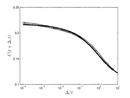
Fig. 1 shows the sigmoidal behavior of the position autocorrelation function. It is important to note that Eq. (19) implies that the process is irreversible since in the limit $\Delta\to\infty$ $B(t\big{/}t+\Delta,\alpha,1-\alpha)\to 0$ and $\langle x(t_{2})x(t_{1})\rangle\to\langle x\rangle_{B}^{2}$.

Figure 1: Position correlation correlation function $C(t_{2},t_{1})=\langle x(t_{2})x(t_{1})$ from Eq. (19) (solid line) as function of the scaled time $\Delta/t$ for $\alpha=0.525$, where $\Delta=|t_{2}-t_{1}|$. The values of the Boltzmann moments are $\langle x^{2}\rangle_{B}=0.217$ and $\langle x\rangle_{B}^{2}=0.102$. We also show data ($\circ$ symbols) for the magnetization $M(t+\Delta,t)$ from the thermoremanent magnetization experiment reported in Ref. [57] from measurement in a $\text{Cu}_{0.94}\text{Mn}_{0.06}$ sample, showing aging behavior. The shown data correspond to the longest measured waiting time, $t=10000$ sec.

The result (19) has some remarkable properties. Thus the external potential $U(x)$ enters only via the prefactor, and only through the first two moments of the corresponding Boltzmann distribution. The long time behavior of $\langle x(t_{2})x(t_{1})\rangle$ is universal and depends only on the ratio $t_{2}/t_{1}$.

We note that Beta function behavior for a correlation function was found previously for a simple two-state renewal model with power-law sojourn times on both states [3, 20, 22, 23, 54, 55]. While our process is clearly not a two state process, the universal behavior of expression (19) is due to the separation between the physical process in space and the associated temporal process. Such a separation is exactly the idea behind the subordination of time, Eq. (12)(b). The temporal process $t(s)$ yields the time evolution governed by the waiting times between successive jumps. Due to the assumption of annealed disorder it is independent of the current particle position. It converges as a function of the number of jumps ($\propto s$) due to the generalized central limit theorem, corresponding to the long-time limit $s\to\infty$ in Eq. (12)(b). The limiting behavior of $t(s)$ is therefore a Lévy stable law which is underlying the subdiffusion dynamics. Conversely, the spatial process explores the external potential and is not affected by the disorder if observed as a function of the internal time $s$. In fact, as function of $s$ the process corresponds to normal diffusion in an external field, and so the process converges to Boltzmann statistics characterised by the binding properties of the external potential. We note that the result (19) for the correlation function mirrors the convergence of both temporal and spatial processes, and is independent of the microscopic properties of the model (e.g. the shape of $U(x)$). To obtain the behavior when one of the processes has not converged one needs to use the full correlation function with a non-trivial time dependence [52]. The latter depends on all eigen-values of $\mathbb{L}_{\mathrm{FP}}$ and is cumbersome.

2.2 Properties of the two-time position correlation

The correlation function (19) displays a number of noteworthy features:

2.2.1 (i) Aging behavior

The correlation function $C(t+\Delta,t)=\langle x(t+\Delta)x(t)\rangle$ exhibits aging since its time dependence is of the form $\Delta/t$. Aging behavior was indeed observed in many complex systems [3, 16, 57], for instance, in thermoremanent magnetization experiments [56, 57], in which the measured relaxation of the magnetization $M(t+\Delta,t)$ is proportional to the spin correlation function, according to generalized fluctuation-dissipation theorems [58, 55, 3]. Accepting our stochastic theory as an approximation for the spin system behavior we used Eq. (19) to fit the thermoremanent magnetization data from Ref. [57]. The result of the fit is presented in Fig. 1. We observe good agreement between the data and our Beta function results over the entire time window, with a slight discrepancy at short times. We note that the use of a non-zero value for the fitting parameter $\langle x\rangle_{B}^{2}$ in Eq. (19) for the zero external field relaxation of the magnetization is consistent with observed asymmetric magnetic fluctuations in thermoremanent magnetization experiments [59] as opposed to the naively expected zero average behavior. Fitting with the Beta function for the measured correlation function does not necessarily yield insight into the physics of the system, but classification of aging with particular fitting functions might be profitable step (as the well known functions, such as Cole-Cole plots, are useful in the classification of dielectric relaxation).

2.2.2 (ii) Time-averaged position

We quantify ergodicity, or the departure from ergodicity, of the system by measuring fluctuations of the time averaged position

$$\overline{x(t)}=\frac{1}{t}\int_{0}^{t}x(t^{\prime})\,dt^{\prime}.$$ (22)

Combining Eqs. (5) and (19) we see that

$$\lim_{t\to\infty}\left<\overline{x(t)}^{2}\right>=(1-\alpha)(\langle x^{2}\rangle_{B}-\langle x\rangle_{B}^{2})+\langle x\rangle_{B}^{2},$$ (23)

where we used the relation

$$\int_{0}^{1}B(z,\alpha,1-\alpha)dz=(1-\alpha)\Gamma(\alpha)\Gamma(1-\alpha).$$ (24)

This result was previously obtained for a CTRW process [60]. Clearly $\left<\overline{x(t)}^{2}\right>\neq\langle x\rangle_{B}^{2}$ when $\alpha<1$, thus we observe weakly non-ergodic behavior. In the limit $\alpha=1$ ergodicity is restored.

2.2.3 (iii) Edwards-Anderson parameter

The Edwards-Anderson parameter was previously used to quantify the degree of weak ergodicity breaking in the context of spin-glasses [3]. It is defined as

$$q_{EA}=\lim_{\Delta\to\infty}\lim_{t\to\infty}C(t+\Delta,t).$$ (25)

In our current framework, for the case of a symmetric potential the Edwards-Anderson parameter becomes

$$q_{EA}=\left\{\begin{array}[]{ll}\langle x^{2}\rangle_{B},&\alpha<1\\ 0,&\alpha\geq 1\end{array}\right.,$$ (26)

reflecting irreversibility of our process which is still non-ergodic. Conversely, interchanging the limits we find that

$$\lim_{t\to\infty}\lim_{\Delta\to\infty}C(t+\Delta,t)=0.$$ (27)

reflecting the aging character of the system. Note that Eq. (26) indicates that $q_{EA}$ is determined by the Boltzmann distribution and is independent of $\alpha$ in the nonergodic phase.

2.2.4 (iv) Time-averaged mean squared displacement

From Eq. (19) we also obtain the behavior of the ensemble average of the time averaged mean squared displacement [61, 62]. Namely, from a time series $x(t)$ recorded in single particle tracking experiments one can define the time averaged mean squared displacement

$$\overline{\delta^{2}(\Delta)}=\frac{1}{T-\Delta}\int_{0}^{T-\Delta}\Big{[}x(t+\Delta)-x(t)\Big{]}^{2}dt,$$ (28)

where $T$ is the overall measurement time. At finite measurement time $T$ even in the Brownian limit the quantity $\overline{\delta^{2}(\Delta)}$ is a random quantity depending on the particular trajectory. Performing an additional ensemble average, for a Brownian system the role of the lag time $\Delta$ in the long measurement time limit is completely interchangeable with the regular $t$-dependence in the corresponding ensemble averaged mean squared displacement, for example when $U(x)=0$ $\lim_{T\to\infty}\overline{\delta^{2}(\Delta,T)}=2K\Delta$. In presence of a confining potential one would naively expect the mean squared displacement to saturate, as observed for a Brownian system. However, evaluating the ensemble average of $\overline{\delta^{2}(\Delta)}$

$$\left<\overline{\delta^{2}(\Delta)}\right>=\frac{1}{T-\Delta}\int_{0}^{T-\Delta}\left<\Big{[}x(t+\Delta)-x(t)\right]^{2}\Big{>}dt$$

$$=\frac{{\displaystyle\int}_{0}^{T-\Delta}\Big{[}\langle x^{2}(t+\Delta)\rangle+\langle x^{2}(t)\rangle-2C(t+\Delta,t)\Big{]}dt}{T-\Delta}.$$ (29)

we find the a priori surprising result : For regular diffusion in a binding potential one obtains a saturation for long times, as for anomalous motion in the case of the ensemble average [12, 13]. In contrast, for the time averaged mean squared displacement in our anomalous system from Eq. (29) we find from the Beta function expansion

$$\frac{B(t/(t+\Delta),\alpha,1-\alpha)}{\Gamma(\alpha)\Gamma(1-\alpha)}\sim 1-\frac{\sin(\alpha\pi)}{(1-\alpha)\pi}\left(\frac{\Delta}{t}\right)^{1-\alpha}$$ (30)

the behavior

$$\left<\overline{\delta^{2}(\Delta)}\right>\sim\Big{(}\langle x^{2}\rangle_{B}-\langle x\rangle_{B}^{2}\Big{)}\frac{2\sin(\alpha\pi)}{(1-\alpha)\alpha\pi}\left(\frac{\Delta}{T}\right)^{1-\alpha},$$ (31)

valid in the limit $(\Delta/T)\ll 1$ and for $\Delta\gg(1/K_{\alpha}\mu_{1})^{1/\alpha}$ [52]. Instead of the naively expected saturation, the time averaged mean squared displacement grows as a power with exponent $(1-\alpha)$. Only when the lag time approaches the measurement time $T$ this power-law growth stops, and the function dips to the ensemble averaged value. We note that the $\Delta^{1-\alpha}$ scaling was recently reported for the case of a particle in a box [63].

2.2.5 (v) Numerical analysis of position autocorrelation.

Figure 2: Simulated behavior of the time-averaged mean squared displacement $\left<\overline{\delta^{2}(\Delta)}\right>$ for a continuous time random walk process with waiting time distribution $\psi(t)\sim\tau^{\alpha}/t^{1+\alpha}$, in an harmonic binding potential $U(x)=x^{2}$ ($\square$), and in a box with reflecting boundary conditions and size $2$ ($\circ$). The anomalous diffusion exponent is $\alpha=1/2$, and the measurement time was chosen as $T=10^{7}$ (a.u.). We also chose $k_{B}T_{mp}=0.1$, and $K_{1/2}=0.0892$. Without fit, the lines show the analytic results for the transition from the initial linear lag time dependence $\simeq\Delta^{1}$, Eq. (32) (— and $-\cdot-$), to the long lag time behavior $\simeq\Delta^{1-\alpha}$, Eq. (31) (—). In both cases $\langle x\rangle_{B}=0$. At long lag times $\left<\overline{\delta^{2}(\Delta)}\right>/\langle x^{2}\rangle_{B}$ exhibits universal behavior, independent of the external field.

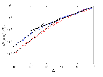
Fig. 2 shows, over a large time span, the time-averaged mean squared displacement $\left<\overline{\delta^{2}(\Delta)}\right>$ of a subdiffusing particle in (i) an harmonic potential, and (ii) in a box with reflecting boundaries. The initial particle position was chosen to be at the bottom of the potential and in the center of the box, respectively. At short lag times $\Delta$ we observe the linear scaling

$$\left<\overline{\delta^{2}(\Delta)}\right>\sim\frac{2K_{\alpha}\Delta}{\Gamma(1+\alpha)T^{1-\alpha}}$$ (32)

with the lag time $\Delta$. In this result only the dependence on the overall measurement time $T$ bears witness to the fact that the underlying stochastic process is subdiffusive. Seemingly paradox, the lag time $\Delta$ enters linearly, in contrast to the associated ensemble averaged mean squared displacement $\langle x^{2}(t)\rangle\sim 2K_{\alpha}t^{\alpha}/\Gamma(1+\alpha)$. However, this is the result of the weak ergodicity breaking of the process, as shown in Refs. [61, 62]. The free particle behavior at short $\Delta$ is an expected result, which can be obtained from scaling arguments or explicitly from the full correlation function [52]: at sufficiently short times the particle does not yet feel the confinement due to the reflecting boundaries, or it does not yet experience the restoring force of the potential, respectively. The $\left<\overline{\delta^{2}(\Delta)}\right>\simeq\Delta$ regime holds for scales of the lag time $\Delta$ that fulfill $K_{\alpha}\Delta^{\alpha}\ll L^{2}$ in the example of the box, where $L$ is the size of the box. For a general confining potential, the turnover time is non-universal and is dependent on all non-zero eigenvalues $\mu_{n}$ of the Fokker-Planck operator $\mathbb{L}_{\mathrm{FP}}$ [40]. Thus, at times $\Delta\gg(1/K_{\alpha}\mu_{1})^{1/\alpha}$ a transition occurs to the $\left<\overline{\delta^{2}(\Delta)}\right>\sim\Delta^{1-\alpha}$ regime, Eq. (31). We stress again that, in contrast to normal diffusion, no saturation is found at long lag times, and $\left<\overline{\delta^{2}(\Delta)}\right>$ continues to grow for any $\Delta<T$. Only as $\Delta$ approaches to the measurement time $T$, we obtain the convergence $\left<\overline{\delta^{2}(\Delta)}\right>\to\langle x^{2}\rangle+\langle x^{2}(0)\rangle$.

Figure 3: Single trajectories for the motion in the harmonic binding potential $U(x)=x^{2}$, for the same parameters as in Fig. 2 (thin lines). The symbols ($\square$) represent the simulations result for $\left<\overline{\delta^{2}(\Delta)}\right>$. The scatter between individual trajectories is distinct and resembles qualitatively typical experimental results [24, 25, 26, 27, 28, 29].

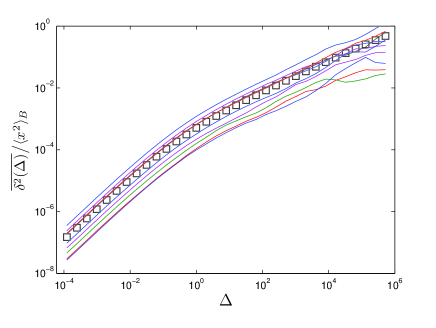
In Fig. 3 we show the simulations result for a number of individual trajectories in an harmonic binding potential, displaying significant scatter. This scatter between individual trajectories is, again, a result of the weak ergodicity breaking of the underlying stochastic process, and resembles qualitatively the behavior observed in single particle tracking experiments [24, 25, 26, 27, 28, 29]. The amplitude of the scatter can be quantified in terms of the dimensionless random variable $\xi\equiv\overline{\delta^{2}(\Delta)}/\left<\overline{\delta^{2}(\Delta)}\right>$, the relative scatter of the time average with respect to its ensemble mean. Using arguments similar to [62] we can show [52] that the distribution of $\xi$ is given in terms of a one-sided Lévy stable law in the form [62]

$$\lim_{T\to\infty}\phi_{\alpha}(\xi)=\frac{\Gamma(1+\alpha)^{1/\alpha}}{\alpha\xi^{1+1/\alpha}}l_{\alpha}\left(\frac{\Gamma(1+\alpha)^{1/\alpha}}{\xi^{1/\alpha}}\right),$$ (33)

where the stable density $l_{\alpha}(t)$ is defined in terms of its Laplace image $\exp(-u^{\alpha})$. Note that the random variable $\xi$ is in the denominator of $l_{\alpha}$, and therefore the associated width is finite. For instance, for the case $\alpha=1/2$ used in Figs. 2 and 3 we find the Gaussian law $\lim_{T\to\infty}\phi_{1/2}(\xi)=(2/\pi)\exp\left(-\xi^{2}/2\right)$. Finally, in the Brownian limit $\alpha=1$, the distribution converges to the sharp behavior $\phi_{1}(\xi)=\delta(\xi-1)$, restoring ergodicity in the sense that no more scatter occurs. The distribution of $\xi$, given by Eq. (33), is the same for both unbounded and bounded anomalous diffusion. This is simply due to the mentioned fact that temporal and spatial process are uncoupled.

3 Discussion

Correlation functions are a standard tool to experimentally probe the temporal evolution of a system. They provide information on how the present value of a physical observable influences its value in the future, and are therefore important indicators to the specific process that governs the system’s dynamics. The significance of the correlation function behavior for the fundamental concepts in physics is revealed through Khinchin’s theorem which provides a condition for a stationary process to be ergodic in terms of the corresponding correlation function. Herein we derived a generalization of Khinchin’s theorem for a class of non-stationary aging process. We provide not only a generalized condition for ergodicity for such processes in terms of the corresponding aging correlation function but also quantify the deviations from ergodicity. For the broad class of non-stationary processes described by Eq. (10) we derived analytically the time dependence of two-point correlation functions for subdiffusing particles under situations of confinement. In particular we revealed a universal behavior for the two-time position correlation function involving the incomplete Beta function. All features of the confining potential enter the correlation function solely through the prefactor in terms of the first and second moments of the associated Boltzmann distribution. Of course, the expression for the correlation function in Eq. (19) is not restricted to a position correlation function, but can be used to describe a very general class of quantities, e.g., a potential energy correlation function. The generality of our results is a direct consequence of the convergence of the Markovian process $x(s)$ in the jump space, and the ubiquitous role of Lévy statistics due to the generalized central limit theorem.

We note that the behavior found for the time-averaged mean squared displacement in binding potential (or confined geometry) recovered herein could be verified in a single particle tracking experiment specifically for micro-movement inside a yeast cell, in which the particle was tracked indirectly in an optical tweezers setup, that eventually exerts a Hookean restoring force on the tracer particle [64]. Similarly anomalous diffusion of macro molecules in a cell is always confined by the cell boundary, indicating that our theory of confined anomalous diffusion may have wide applications.