Embedding realistic surveys in simulations through volume remapping

Abstract

Connecting cosmological simulations to real-world observational programs is often complicated by a mismatch in geometry: while surveys often cover highly irregular cosmological volumes, simulations are customarily performed in a periodic cube. We describe a technique to remap this cube into elongated box-like shapes that are more useful for many applications. The remappings are one-to-one, volume-preserving, keep local structures intact, and involve minimal computational overhead.

1. Introduction

Numerical simulations have become an indispensable tool in modern cosmological research, used for investigating the interplay of complex physical processes, studying regimes of a theory which cannot be attacked analytically, generating high precision predictions for cosmological models, and making mock catalogs for the interpretation and analysis of observations. Such simulations traditionally evolve the matter distribution in periodic cubical volumes, which neatly allow them to approach the homogeneous Friedmann solution on large scales. The use of a periodic volume also allows the long-range force to be easily computed by fast Fourier transform methods in many popular algorithms (e.g. particle-mesh, particle-particle-particle-mesh or tree-particle-mesh algorithms).

Surveys, on the other hand, often cover cosmological volumes that are far from cubical in shape, and making a mock catalog which includes the full geometrical constraints of the observations is difficult. One approach is to simulate a sufficiently large volume that the survey can be embedded directly within the cube, but this often means large parts of the computational domain are unused. An alternative is to trace through the cube across periodic boundaries so as to generate the desired depth, with various rules for avoiding replication or double-counting of the volume (if desired). A third approach is to run a simulation in a non-cubical geometry. If the side lengths are highly disproportionate this can lead to its own numerical issues, and in addition it makes it difficult to reuse a given simulation for many applications.

In this paper we present a new solution to this problem which allows one to embed a hypothetical survey volume inside a cosmological simulation while limiting wasted volume and artificial correlations. The method is based on the simple observations that (1) a cube with periodic boundary conditions is equivalent to an infinite 3-dimensional space with discrete translational symmetry, and (2) the primitive cell for such a space need not be a cube. We show that one may take the primitive cell to be a cuboid of dimensions $L_{1}\times L_{2}\times L_{3}$ for a discrete but large choice of values $L_{1}\geq L_{2}\geq L_{3}$. The possible choices, subject to the constraint $L_{1}L_{2}L_{3}=1$, are illustrated in Figure 1.

Figure 1.— Possible dimensions $L_{1}\times L_{2}\times L_{3}$ for cuboid remappings, subject to the conditions $L_{1}\geq L_{2}\geq L_{3}$, $L_{1}L_{2}L_{3}=1$, and $L_{1}<7$. The choice used for the Stripe 82 remapping described in Section 4 is indicated by a red circle.

Our approach leads to a one-to-one remapping of the periodic cube which keeps structures intact, does not map originally distant pieces of the survey close together, and uses no piece of the volume more than once. It complements existing techniques for generating mock observations (e.g. Blaizot et al. 2005; Kitzbichler & White 2007) or for ray-tracing through simulations (e.g. White & Hu 2000; Vale & White 2003; Hilbert et al. 2009; Fullana et al. 2010). Though not ideal in all cases, our remapping procedure may be seen as a general-purpose alternative that neatly skirts many of the complications involved with previous methods.

We begin in Section 2 with a mathematical description of the remapping, and explain what choices of dimensions are possible. In Section 3 we describe how to implement this remapping numerically. We present a few useful examples in Section 4, and conclude in Section 5 with a discussion of some of the advantages and limitations of this method.

2. Mathematical description

Consider a unit cube with periodic boundary conditions. By tiling copies of this cube in all directions, each point $(x,y,z)\in\mathbb{R}^{3}$ corresponds to a point in the canonical unit cube $[0,1]^{3}$ via the map

$$(x,y,z)\mapsto(x\;\mathrm{mod}\;{1},~{}y\;\mathrm{mod}\;{1},~{}z\;\mathrm{mod}\;{1}),$$ (1)

where “$x\;\mathrm{mod}\;{1}$” is just the fractional part of $x$ if $x\geq 0$, or one minus this fractional part for $x<0$. Since we can identify each point in $\mathbb{R}^{3}$ with a point in $[0,1]^{3}$, any region in space corresponds to a sampling of the unit cube. We are primarily interested in bijective samplings, i.e. regions that according to the above equivalence cover each point of the unit cube once and only once. We call such a sampling a remapping of the unit cube. Equivalently, a remapping may be thought of as a partitioning of the unit cube into disjoint regions, which are then translated by integer offsets and glued back together along periodic boundaries.

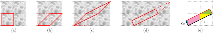
Figure 2.— Panels (a)-(d) show a sequence of shear transformations that results in a remapping of the unit square into a rectangle of dimensions $\sqrt{5}\times 1/\sqrt{5}$, as described in the text. Panel (e) highlights the edge vectors $\bm{e}_{1},\bm{e}_{2}$, and the four cells that comprise this rectangle. Note that each point of the original unit square is covered exactly once in the final remapping.

A general class of such remappings may be constructed by applying shear transformations to the unit cube. We first illustrate the idea in 2D, where the transformations may be easily visualized, and then state the appropriate generalization to 3D. Start with a continuous field laid down within the unit square, which may be thought of as a parallelogram spanned by the vectors $\bm{u}_{1}=(1,0)$ and $\bm{u}_{2}=(0,1)$. We suppose the field to be periodic, and tile copies throughout the plane [see Figure 2(a)]. Now imagine taking the unit square and shearing it along its top edge, leaving the underlying field in place [Figure 2(b)]. The result is a new parallelogram defined by the vectors

$$\bm{u}_{1}=(1,0),\qquad\bm{u}_{2}^{\prime}=\bm{u}_{2}+m\bm{u}_{1}=(m,1),$$ (2)

where $m$ is some real scalar that controls the extent of the shear. Since shear transformations are area-preserving, this parallelogram has unit area. In fact, since $\bm{u}_{1}$ is a lattice vector (i.e. a vector of translational invariance), this parallelogram covers each point of our field once and only once, and hence defines a valid remapping.

Now observe that if $m$ is an integer, then $\bm{u}_{2}^{\prime}=(m,1)$ will also be a lattice vector. In that case we again have a parallelogram with edge vectors $\bm{u}_{1}$ and $\bm{u}_{2}^{\prime}$ that are both lattice vectors. We can now shear this parallelogram along its right edge [Figure 2(c)], giving a new parallelogram with edge vectors

$$\bm{u}_{1}^{\prime}=\bm{u}_{1}+n\bm{u}_{2}^{\prime}=(1+mn,n),\qquad\bm{u}_{2}^{\prime}=(m,1).$$ (3)

Once again this parallelogram covers each point of our field exactly once, and if $n$ is an integer then $\bm{u}_{1}^{\prime}$ and $\bm{u}_{2}^{\prime}$ are both lattice vectors. We may repeat this process, applying integer shears alternately to the top and right edges of the parallelogram. In general, if $\bm{u}_{1}$ and $\bm{u}_{2}$ are any integer-valued 2D vectors that span a parallelogram of unit area, they can be obtained by such a sequence of shear transformations. This condition is simply

$$u_{11}u_{22}-u_{12}u_{21}=\det\begin{pmatrix}u_{11}&u_{12}\\ u_{21}&u_{22}\end{pmatrix}=1,$$ (4)

i.e. $\bm{u}_{1}$ and $\bm{u}_{2}$ are the rows of an invertible integer-valued matrix.

While remapping the unit square into a parallelogram may be useful in certain cases, parallelograms are generally too awkward to be useful. Instead, given lattice vectors $\bm{u}_{1}$ and $\bm{u}_{2}$ spanning unit area, we may apply one last shear to “square up” the parallelogram into a rectangle [Figure 2(d)]. Explicitly, we let

$$\bm{e}_{1}=\bm{u}_{1},\qquad\bm{e}_{2}=\bm{u}_{2}+\alpha\bm{u}_{1},$$ (5)

and choose $\alpha$ so that $\bm{e}_{1}$ and $\bm{e}_{2}$ are orthogonal. The rectangle defined by $\bm{e}_{1}$ and $\bm{e}_{2}$ now covers each point of the unit square exactly once.

The generalization to 3D is straightforward. By applying integer shears to the faces of the cube, we may obtain any parallelepiped with edges given by integer vectors $\bm{u}_{1}$, $\bm{u}_{2}$, $\bm{u}_{3}$ satisfying

$$\det\begin{pmatrix}u_{11}&u_{12}&u_{13}\\ u_{21}&u_{22}&u_{23}\\ u_{31}&u_{32}&u_{33}\end{pmatrix}=1.$$ (6)

Again this space of possibilities corresponds to the space of invertible, integer-valued $3\times 3$ matrices. We apply two final shears to square up this parallelepiped into a cuboid, by choosing coefficients $\alpha$, $\beta$, and $\gamma$ such that

$$\bm{e}_{1} =\bm{u}_{1},$$ (7)

$$\bm{e}_{2} =\bm{u}_{2}+\alpha\bm{u}_{1},$$ (8)

$$\bm{e}_{3} =\bm{u}_{3}+\beta\bm{u}_{1}+\gamma\bm{u}_{2},$$ (9)

are mutually orthogonal. This gives a remapping of the unit cube into a cuboid with side lengths $L_{i}=|\bm{e}_{i}|$, satisfying $L_{1}L_{2}L_{3}=1$. Moreover since $\bm{e}_{1}$ is still a lattice vector, this cuboid is periodic across the face perpendicular to this vector.

Invertible, integer-valued $3\times 3$ matrices can be generated easily by brute force computation, and each such matrix leads to a cuboid remapping of the unit cube. The allowable dimensions $L_{1}\times L_{2}\times L_{3}$ for these cuboids are illustrated in Figure 1, where $L_{3}$ is given implicitly by the unit volume condition $L_{1}L_{2}L_{3}=1$.

3. Numerical algorithm

The goal of our remapping procedure is to provide an explicit bijective map between the unit cube and a cuboid of dimensions $L_{1}\times L_{2}\times L_{3}$. We will refer to points in the unit cube by their simulation coordinates $\bm{x}\in[0,1]^{3}$, and their remapped positions in a canonical, axis-aligned cuboid by remapped coordinates $\bm{r}\in[0,L_{1}]\times[0,L_{2}]\times[0,L_{3}]$.

The reverse map $\bm{r}\mapsto\bm{x}$ is simple. The edge vectors $\bm{e}_{1},\bm{e}_{2},\bm{e}_{3}$ discussed previously describe how to embed an oriented cuboid within an infinite tiling of the unit cube. Let $\hat{n}_{i}=\bm{e}_{i}/L_{i}$ be unit vectors along these edges. Then given $(r_{1},r_{2},r_{3})\in[0,L_{1}]\times[0,L_{2}]\times[0,L_{3}]$, the point

$$\bm{p}=r_{1}\hat{n}_{1}+r_{2}\hat{n}_{2}+r_{3}\hat{n}_{3}$$ (10)

lies within this oriented cuboid, and this maps to a point in the unit cube according to Eq. (1).

The forward map $\bm{x}\mapsto\bm{r}$ is slightly more complicated. Consider again the oriented cuboid with edge vectors $\bm{e}_{1},\bm{e}_{2},\bm{e}_{3}$ embedded within an infinite tiling of the unit cube. Each tile (i.e. each replication of the unit cube) may be labeled naturally by an integer triplet $\bm{m}\in\mathbb{Z}^{3}$, where the canonical unit cube has $\bm{m}=(0,0,0)$. The intersection of the cuboid with a tile is called a cell, of which only a finite number will be non-empty. Each non-empty cell is uniquely labeled by the triplet $\bm{m}$. [The four cells of the 2D example from the previous section are indicated in Figure 2(e).]

As a geometrical object, each cell is just a convex polyhedron bounded by 12 planes: the 6 faces of the tile and the 6 faces of the cuboid. A plane may be parametrized by real numbers $(a,b,c,d)$, so that a point $(x,y,z)$ lies inside, outside, or on the plane depending on whether the quantity $ax+by+cz+d$ is less than, greater than, or equal to zero. Thus to test whether a point belongs to a cell, we need only check if it lies inside all the planes that bound it. When translated spatially by a displacement $-\bm{m}$, each cell defines a region within the unit cube. The collection of all such cells defines a partitioning of the unit cube, with each point in $[0,1]^{3}$ being covered by exactly one cell. Our algorithm for the forward map $\bm{x}\mapsto\bm{r}$ then may be summarized as follows:

1. determine which cell contains the point $\bm{x}$ (using point-plane tests)

2. let $\bm{p}=\bm{x}+\bm{m}$ be the corresponding point in the oriented cuboid

3. define $\bm{r}\in[0,L_{1}]\times[0,L_{2}]\times[0,L_{3}]$ by $r_{i}=\bm{p}\cdot\hat{n}_{i}$

4. Examples and applications

The mappings described above can be used in myriad ways. The algorithm is fast enough that it can be used for on-the-fly analysis while a simulation is running, it introduces little overhead in walking a merger tree (allowing complex light-cone outputs to be built during e.g. the running of a semi-analytic galaxy formation code), or it can be applied in post-processing to a static time output of a simulation to alter the geometry. In this section we give a (very) few illustrative examples.

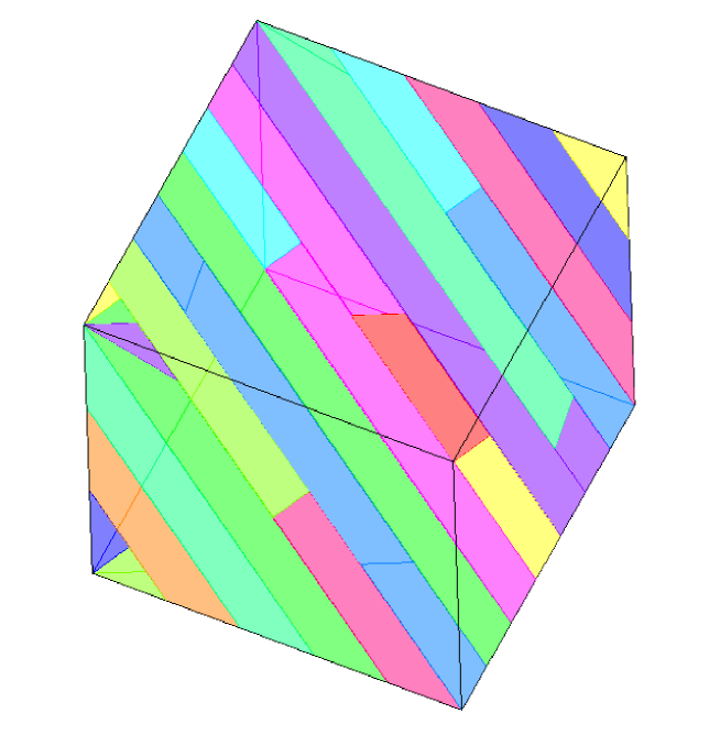
Figure 3.— The regions in the unit cube, and how they “unfold” to produce the wide, thin geometry shown in Figure 4.

As it is so widely known we shall use as our fiducial volume the Millennium simulation (Springel et al., 2005), which was performed in a cubical volume of side length $500\,h^{-1}$Mpc. We begin by asking how we could embed a very wide-angle survey, such as the equatorial stripe (“Stripe 82”) of the Sloan Digital Sky Survey, in such a volume. Stripe 82 is $100^{\circ}$ wide and $2.5^{\circ}$ in height. Using the Millennium simulation cosmology, the volume within Stripe 82 out to $z\simeq 0.45$ equals the total volume within the Millennium simulation. At this depth the stripe is $1.2\,h^{-1}$Gpc in the line-of-sight direction, $1.9\,h^{-1}$Gpc transverse but only $50\,h^{-1}$Mpc deep.

We can map the cubical volume of the simulation into this geometry using the transformation circled in red in Fig. 1. A view of this transformation is given in Figure 3, where the regions within the cube are shown “unfolded” to produce a long and wide, but thin, domain into which we can embed the Stripe 82 geometry. Figure 4 shows a light-cone produced from the outputs of the Millennium simulation, in the Stripe 82 geometry. Specifically we show all galaxies brighter than $R=-20.5$ (to avoid saturating the figure) and with $0<z<0.45$ from the catalog of De Lucia & Blaizot (2007).

Figure 4.— A mock catalog from the Millennium simulation remapped into the equatorial stripe of the Sloan Digital Sky Survey. The “stripe” is a thin rectangle on the sky of angular dimensions $100^{\circ}\times 2.5^{\circ}$, shown here “from above” extending out to redshift $z\simeq 0.45$, or $r\simeq 1.2\,h^{-1}$Gpc comoving. We show only galaxies brighter than $R=-20.5$, to avoid saturating the figure.

Another frequently encountered situation is a survey which is much longer in the line-of-sight direction than either of the (approximately equal) transverse directions. Let us consider for example a survey which aims to reach $z\simeq 3$, or about $5\,h^{-1}$Gpc in the Millennium simulation cosmology. Among the many possible choices at our disposal we find a remapping with $(L_{1},L_{2},L_{3})=(5025,179,139)\,h^{-1}$Mpc, which could encompass a survey of angular dimensions $2.0^{\circ}\times 1.6^{\circ}$ out to $z\simeq 3.5$. To probe even earlier epochs we could choose a remapping with $(L_{1},L_{2},L_{3})=(7106,145,121)\,h^{-1}$Mpc, which allows a $1.2^{\circ}\times 1.0^{\circ}$ survey out to $z\simeq 10$. For these types of highly elongated geometries, the possible remappings are dense enough that a suitable choice may be found for almost any survey.

5. Discussion

As surveys become increasingly complex and powerful and the questions we ask of them become increasingly sophisticated, mock catalogs and simulations which can mimic as much as possible the observational non-idealities become increasingly important. Angulo & White (2009) have shown that simulations of one cosmology can be rescaled to approximate those of a different cosmology. We have introduced a remapping of periodic simulation cubes which allows one simulation to take on the characteristics of many different observational geometries. The use of such techniques enhances the usefulness of cosmological simulations, which often involve a large investment of community resources.

The methods we introduced in this paper lead to one-to-one remappings of the periodic cube which keep structures intact, do not map originally distant pieces of the survey close together, and use no piece of the volume more than once. The remapping can be done extremely quickly, meaning it can be included in almost any analysis tool with negligible overhead.

Remapping the computational geometry is, however, not without its limitations. First and foremost, although the target geometry may have sides much longer than the original simulation, the structures will not contain the correct large scale power since it was missing from the simulation to begin with. This problem becomes less acute as the original simulation volume becomes a fairer representation of the Universe. Secondly, if the target geometry is too thin it is possible for points which are far apart in the survey to come from points close together in the simulation volume, leading to spurious correlations. These are analogous to the artificial correlations between survey “sides” that occur when it is embedded in a periodic cube. Simply excluding a boundary layer from the remapped volume can tame such correlations.

In addition to the description of the algorithm in this paper, we have made Python and C++ implementations of the remappings, along with further examples and animations, publicly available at http://mwhite.berkeley.edu/BoxRemap.

References

- Angulo & White (2009) Angulo, R. E., & White, S. D. M. 2009, ArXiv e-prints
- Blaizot et al. (2005) Blaizot, J., Wadadekar, Y., Guiderdoni, B., Colombi, S. T., Bertin, E., Bouchet, F. R., Devriendt, J. E. G., & Hatton, S. 2005, MNRAS, 360, 159
- De Lucia & Blaizot (2007) De Lucia, G., & Blaizot, J. 2007, MNRAS, 375, 2
- Fullana et al. (2010) Fullana, M. J., Arnau, J. V., Thacker, R. J., Couchman, H. M. P., & Sáez, D. 2010, ArXiv e-prints
- Hilbert et al. (2009) Hilbert, S., Hartlap, J., White, S. D. M., & Schneider, P. 2009, A&A, 499, 31
- Kitzbichler & White (2007) Kitzbichler, M. G., & White, S. D. M. 2007, MNRAS, 376, 2
- Springel et al. (2005) Springel, V., White, S. D. M., Jenkins, A., Frenk, C. S., Yoshida, N., Gao, L., Navarro, J., Thacker, R., Croton, D., Helly, J., Peacock, J. A., Cole, S., Thomas, P., Couchman, H., Evrard, A., Colberg, J., & Pearce, F. 2005, Nature, 435, 629
- Vale & White (2003) Vale, C., & White, M. 2003, ApJ, 592, 699
- White & Hu (2000) White, M., & Hu, W. 2000, ApJ, 537, 1