CURVATURE AND TOPOLOGICAL EFFECTS ON DYNAMICAL SYMMETRY BREAKING IN A FOUR- AND EIGHT-FERMION INTERACTION MODEL

Abstract

A dynamical mechanism for symmetry breaking is investigated under the circumstances with the finite curvature, finite size and non-trivial topology. A four- and eight-fermion interaction model is considered as a prototype model which induces symmetry breaking at GUT era. Evaluating the effective potential in the leading order of the $1/N$-expansion by using the dimensional regularization, we explicitly calculate the phase boundary which divides the symmetric and the broken phase in a weakly curved space-time and a flat space-time with non-trivial topology, $R^{D-1}\otimes S^{1}$.

1 Introduction

It is believed that a fundamental theory with a higher symmetry is realized at high energy scale. In a grand unified theory, the higher gauge symmetry is broken down to the standard model gauge symmetry, $SU_{c}(3)\otimes SU(2)_{L}\otimes U(1)_{Y}$. The evolution of the universe has played an important role for the symmetry breaking. On the other hand the symmetry breaking affects the space-time structure of the universe. Therefore it is expected that some evidences of symmetry breaking at GUT era will be observed in the structure of the current universe.

One of the well-known mechanism of the symmetry breaking is found for the chiral symmetry breaking in QCD. Below the QCD scale a composite operator which is constructed by quark and anti-quark fields develops a non-vanishing expectation value and the quark fields acquire mass term. Then the chiral symmetry is spontaneously broken. It is caused by non-perturbative effect of QCD dynamics and called as dynamical symmetry breaking. This mechanism can be applied to strong coupling gauge theories at GUT scale.

Thus we have launched our plan for a systematic study on the dynamical symmetry breaking in extreme conditions at the early universe. A simple four-fermion interaction model are often used for the analysis of the dynamical symmetry breaking. The curvature effects has been studied in two[3, 4], three[6], four[5] and arbitrary dimensions.[7]. If the background space-time has a positive curvature, the symmetry breaking is suppressed. The broken symmetry is restored for a large positive curvature, while only the broken phase can be realized in a space-time with a negative curvature.[8] The finite size effect has been investigated in the cylindrical universe,[9] and the torus universe.[10, 11, 12, 13, 14] The finite size effect restore the broken symmetry if we adopt the anti-periodic boundary condition to the fermion fields. The fermion fields with the periodic boundary condition breaks the chiral symmetry. A combined effect of the space-time curvature and the topology has been also discussed in a weakly curved space-time,[18] the maximally symmetric space-time[15, 16] and Einstein space[17, 19]. For a review, see for example Ref. [20].

Strong gauge interactions at high energy scale can be represented by various operators in low energy effective models. It is not always valid to neglect higher dimensional operators. ’t Hooft introduced a determinantal interactions in a low energy effective model of QCD to deal with the explicit breaking of the $U_{A}(1)$ symmetry.[21] R. Alkofer and I. Zahed considered an eight-fermion interaction to explain the pseudoscalar nonet mass spectrum.[22] An influence of higher derivatives is also considered in Ref. [23].

In the present paper we consider four- and eight-fermion interactions and investigate the phase structure of the model in a weakly curved space-time and a space-time with non-trivial topology. In Sec. 2 we introduce a four- and eight-fermion interaction model and calculate the effective potential in the leading order of the $1/N$ expansion. In Sec. 3 we discuss the curvature effect on the dynamical symmetry breaking. It is assumed that the space-time curves slowly. We keep only terms independent of the space-time curvature $R$ and linear to $R$ and study the curvature induced phase transition. We consider a cylindrical universe, $R^{D-1}\otimes S^{1}$ in Sec. 4. It is a flat space-time with non-trivial topology. We adopt a periodic and an anti-periodic boundary conditions for the fermion fields. The phase structure of the model is studied as the size for $S^{1}$ direction varies for each boundary conditions. In Sec. 5 we give some concluding remarks.

2 Four- and Eight-Fermion Interaction Model

The space-time structure modifies the phase structure of the four-fermion interaction model.[20] The simplest model is composed of $N$-flavor fermions with a scalar type four-fermion interaction. In an extreme conditions some interactions described by higher dimensional operators may have nonnegligible contribution to the phase structure. Thus we extend the model with higher dimensional operators to find a general and an essential feature for the dynamical symmetry breaking. We employ scalar type four- and eight-fermion interactions in a curved space-time and start from the action,

$$S = \int d^{D}x\sqrt{-g}\left[\sum_{i=1}^{N}\bar{\psi}_{i}(x)i\gamma^{\mu}(x)\nabla_{\mu}\psi_{i}(x)+\frac{G_{1}}{N}(\sum_{i=1}^{N}\bar{\psi}_{i}(x)\psi_{i}(x))^{2}\right.$$ (1)

$$\left.+\frac{G_{2}}{N^{3}}(\sum_{i=1}^{N}\bar{\psi}_{i}(x)\psi_{i}(x))^{4}\right],$$

where the index $i$ represents the flavors of the fermion field $\psi$, $N$ is the number of flavors, $g$ the determinant of the metric tensor, $\gamma^{\mu}(x)$ the Dirac matrix in curved space-time and $\nabla_{\mu}\psi$ the covariant derivative for the fermion field $\psi$. The coupling constants for the four- and the eight-fermion interactions, $G_{1}$ and $G_{2}$, should be fixed phenomenologically. Since the model is unrenormalizable, we need one more parameter to regularize radiative corrections. In this paper we adopt the dimensional regularization for fermion loop corrections. We leave the space-time dimension, $D$, as an arbitrary parameter to be fixed phenomenologically.[31, 32, 33, 34, 35]

The action (1) is a simple extension of the Gross-Neveu model[2] with the same symmetry. It is invariant under the discrete chiral transformation,

$$\bar{\psi}_{i}\psi_{i}\rightarrow-\bar{\psi}_{i}\psi_{i},$$ (2)

and the global flavor transformation,

$$\psi_{i}\rightarrow\left(\exp(i\sum_{a}\theta_{a}T_{a})\right)_{ij}\psi_{j},$$ (3)

where $T_{a}$ are generators of the flavor $SU(N)$ symmetry. The flavor symmetry allows us to work in a scheme of the $1/N$ expansion. Below we neglect the flavor index.

The generating functional of the model is given by

$$Z=\int{\cal D}\psi{\cal D}\bar{\psi}e^{iS}.$$ (4)

It should be noted that we set the path integral measure to keep the general covariance. For practical calculations it is more convenient to introduce the auxiliary fields. We consider a constant integral,

$$C=\int D\sigma\delta\left(\sigma+\frac{2G_{1}}{N}\bar{\psi}\psi\right).$$ (5)

The delta function in Eq.(5) is described by the integral form,

$$C=C^{\prime}\int D\sigma Dse^{iS_{a}},$$ (6)

where $S_{a}$ is given by

$$S_{a}=i\int\sqrt{-g}d^{D}x\left[-\frac{N}{2G_{1}}s\left(\sigma+\frac{2G_{1}}{N}\bar{\psi}\psi\right)\right].$$ (7)

Since $C$ is a constant, we are free to insert it on the right-hand side in Eq.(4). The fermion bilinear, $\bar{\psi}\psi$, is replaced by the auxiliary field $\sigma$. Thus the generating functional, $Z$, is rewritten as

$$Z=\int D\psi D\bar{\psi}D\sigma Dse^{iS_{y}},$$ (8)

where $S_{y}$ is given by

$$S_{y} = S+S_{a}$$ (9)

$$= \int d^{D}x\sqrt{-g}\left[\bar{\psi}(i\gamma^{\mu}(x)\nabla_{\mu}-s)\psi+\frac{N}{4G_{1}}\sigma^{2}-\frac{N}{2G_{1}}s\sigma+\frac{NG_{2}}{16G_{1}^{4}}\sigma^{4}\right].$$

The eight-fermion interactions in the original action are replaced by the auxiliary fields, $s$ and $\sigma$.

From the action (9) we obtain the equations of motion for the auxiliary fields,

$$\sigma=-\frac{2G_{1}}{N}(\bar{\psi}\psi),$$ (10)

and

$$s=\sigma+\frac{G_{2}}{2G_{1}^{3}}\sigma^{3}.$$ (11)

If a non-vanishing expectation value is assigned for the auxiliary field, $\sigma$, the composite operator, $\bar{\psi}\psi$, also has a non-vanishing expectation value and the chiral symmetry is eventually broken. A non-vanishing expectation value for the auxiliary field, $s$, generates the fermion mass term. Substituting the equations (10) and (11) into the action (9), we can reproduce the original one (1).

For later convenience we shift the field $\sigma$ to $\sigma^{\prime}\equiv\sigma-s$ and diagonalize the mass term for the auxiliary fields. Thus the action (9) reads

$$S_{y}=\int d^{D}x\sqrt{-g}\left[\bar{\psi}(i\gamma^{\mu}(x)\nabla_{\mu}-s)\psi+\frac{N}{4G_{1}}\sigma^{\prime 2}-\frac{N}{4G_{1}}s^{2}+\frac{G_{2}N}{16G_{1}^{4}}(\sigma^{\prime}+s)^{4}\right].$$ (12)

To include quantum corrections we calculate the effective action. Performing the path-integral over the fermion fields, we calculate the effective action $\Gamma[s,\sigma^{\prime}]$ in the leading order of the $1/N$ expansion,

$$\Gamma[s(x),\sigma^{\prime}(x)] = \int d^{D}x\sqrt{-g}\left[\frac{N}{4G_{1}}\sigma^{\prime 2}-\frac{N}{4G_{1}}s^{2}+\frac{NG_{2}}{16G_{1}^{4}}(\sigma^{\prime}+s)^{4}\right]$$ (13)

$$+i\mbox{Tr}\int_{0}^{s}dmS(x,x;m),$$

where Tr represents the trace over the flavor, spinor and space-time coordinates. We want to find a ground state of the system described by the action (12). We assume that the ground state is static and homogeneous and put $s(x)=s$ and $\sigma(x)=\sigma$ constants independent of the space-time coordinate $x$. Then we can obtain the effective potential,

$$V(s,\sigma^{\prime})=-\frac{1}{4G_{1}}\sigma^{\prime 2}+\frac{1}{4G_{1}}s^{2}-\frac{G_{2}}{16G_{1}^{4}}(\sigma^{\prime}+s)^{4}-i\mbox{tr}\int_{0}^{s}dmS(x,x;m),$$ (14)

where tr shows the trace over only the spinor and we omit the over all factor $N$. $S(x,y;m)$ is the spinor two-point function which satisfies the Dirac equation in curved space-time,

$$(i\gamma^{\mu}\nabla_{\mu}-m)S(x,y;m)=\frac{1}{\sqrt{-g}}\delta^{D}(x-y).$$ (15)

The effective potential (14) gives the energy density induced by the fermion fields. The ground state have to minimize it. Thus we can find the state by the stationary condition of the effective potential,

$$\left.\frac{\partial V(s,\sigma^{\prime})}{\partial s}\right|_{\sigma^{\prime}}=\frac{s}{2G_{1}}-\frac{G_{2}}{4G_{1}^{4}}(\sigma^{\prime}+s)^{3}-i\mbox{tr}S(x,y;s)=0$$ (16)

and

$$\left.\frac{\partial V(s,\sigma^{\prime})}{\partial\sigma^{\prime}}\right|_{s}=-\frac{\sigma^{\prime}}{2G_{1}}-\frac{G_{2}}{4G_{1}^{4}}(\sigma^{\prime}+s)^{3}=0.$$ (17)

Eqs. (16) and (17) give necessary conditions for the minimum. From Eq.(17) we get

$$s=\left(-\frac{2G_{1}^{3}}{G_{2}}\sigma^{\prime}\right)^{1/3}-\sigma^{\prime}.$$ (18)

In terms of the auxiliary field, $\sigma=s+\sigma^{\prime}$, the equation reads

$$s=\sigma+\frac{G_{2}}{2G_{1}^{3}}\sigma^{3}.$$ (19)

This equations give the relationship between both the auxiliary fields at the stationary point. Thus the dynamical fermion mass, $m_{d}\equiv\langle s\rangle$ is given by a function of $\langle\sigma\rangle\propto\langle\bar{\psi}\psi\rangle$. Substituting Eq. (19) into Eq. (16), we obtain

$$s=i2G_{1}\mbox{tr}S(x,x;s)-4iG_{2}\left[\mbox{tr}S(x,x;s)\right]^{3}.$$ (20)

The dynamically generated fermion mass, $m_{d}$, should satisfy this gap equation. In the case of the second order phase transition the dynamical fermion mass smoothly disappears at the critical point. We can calculate it to take the limit $s\rightarrow 0$ for the non-trivial solution of Eq. (20). Because of the chiral symmetry tr$S(x,x;s)$ is proportional to $s$. Thus the second term in the right-hand side in Eq. (20) drops much faster than the other terms. It shows that the eight-fermion interaction $G_{2}$ has nothing to do with the critical point for the second order phase transition.

We can obtain the self-consistent equation (20) for the dynamically generated fermion mass in other procedures. An alternative way is possible to cancel out multi-fermion interactions by introducing the auxiliary fields. In Ref. [30] the action (1) is rewritten by the auxiliary fields $\sigma_{1}$ and $\sigma_{2}$,

$$S_{y}^{\prime}=\int d^{D}x\sqrt{-g}\left[\bar{\psi}(i\gamma^{\mu}(x)\nabla_{\mu}-\sigma_{f})\psi-\frac{N\sigma_{1}^{2}}{4G_{1}}-\frac{N\sigma_{2}^{2}}{4G_{2}}\right],$$ (21)

where $\sigma_{f}$ is given by

$$\sigma_{f}\equiv\sigma_{1}\sqrt{1-\frac{\sigma_{2}}{G_{1}}}.$$ (22)

In terms of the auxiliary fields $\sigma_{1}$ and $\sigma_{2}$ the effective potential is found to be

$$V(\sigma_{1},\sigma_{2})=\frac{1}{4G_{1}}\sigma_{1}^{2}+\frac{1}{4G_{2}}\sigma_{2}^{2}-i\mbox{tr}\int_{0}^{\sigma_{f}}dmS(x,x;m).$$ (23)

From the stationary condition of the effective potential (23) we obtain the self-consistent equation for the dynamically generated fermion mass,

$$\sigma_{f}=i2G_{1}\mbox{tr}S(x,x;\sigma_{f})-4iG_{2}\left[\mbox{tr}S(x,x;\sigma_{f})\right]^{3}.$$ (24)

It is equivalent to the gap equation (20).

We can also derive the fermion mass from the original action (1). In the leading order of the $1/N$ expansion it is given by the following diagrams,

$$m_{d} = \mbox{ \begin{minipage}{56.9055pt} \hskip 2.84526pt \includegraphics[height=22.76219pt]{2fG1.eps} \end{minipage} }+\mbox{ \begin{minipage}{56.9055pt} \hskip 2.84526pt \includegraphics[height=36.98857pt]{2fG2.eps} \end{minipage} }$$ (25)

$$= 2iG_{1}\mbox{tr}S(x,x;m_{d})-4iG_{2}\left(\mbox{tr}S(x,x;m_{d})\right)^{3}.$$

Therefore the gap equation (20) is reproduced again.

Before we discuss the curvature and the topological effect, it will be instructive to give the type behavior of the effective potential Eq. (14) in Minkowski space-time, $R^{D}$. The two-point function (15) in $R^{D}$ is given by

$$S(x,y;s)=\int\frac{d^{D}k}{(2\pi)^{D}}e^{-ik(x-y)}\frac{1}{\gamma^{\mu}k_{\mu}-s}.$$ (26)

Inserting Eq.(26) into Eq.(14), we obtain the explicit expression for the effective potential,

$$V_{0}(s,\sigma^{\prime}) = -\frac{1}{4G_{1}}\sigma^{\prime 2}+\frac{1}{4G_{1}}s^{2}-\frac{G_{2}}{16G_{1}^{4}}(\sigma^{\prime}+s)^{4}$$ (27)

$$-\frac{\mbox{tr1}}{(4\pi)^{D/2}D}\Gamma\left(1-\frac{D}{2}\right)|s|^{D}.$$

At the stationary point, the effective potential is rewritten as

$$V_{0}(\sigma) = \frac{1}{4G_{1}}\left(\sigma^{2}+\frac{3G_{2}}{4G_{1}^{3}}\sigma^{4}\right)$$ (28)

$$-\frac{\mbox{tr1}}{(4\pi)^{D/2}D}\Gamma\left(1-\frac{D}{2}\right)\left|\sigma+\frac{G_{2}}{2G_{1}^{3}}\sigma^{3}\right|^{D}.$$

In $R^{D}$ the gap equation (20) is given by

$$s=2G_{1}\frac{\mbox{tr}1}{(4\pi)^{D/2}}\Gamma\left(1-\frac{D}{2}\right)s|s|^{D-2}+4G_{2}\left[\frac{\mbox{tr}1}{(4\pi)^{D/2}}\Gamma\left(1-\frac{D}{2}\right)s|s|^{D-2}\right]^{3}.$$ (29)

For $G_{2}=0$ we can analytically solve this gap equation and find a non-trivial solution for a negative $G_{1}$ at

$$s=\sigma=m_{0}\equiv\left[-\frac{(4\pi)^{D/2}}{2|G_{1}|\mbox{tr}1\Gamma\left(1-D/2\right)}\right]^{1/(D-2)}.$$ (30)

This solution gives the dynamically generated fermion mass for $G_{2}=0$ in $R^{D}$. Below we normalize all the mass scales by $m_{0}$ for $G_{1}<0$. In the case of a positive $G_{1}$ we also use $m_{0}$ to normalize parameters with mass dimension. Thus the effective potential (28) depends on $\sigma$, $D$, a sign of $G_{1}$ and $G_{r}\equiv G_{2}m_{0}^{2}/G_{1}^{3}$,

$$\frac{V_{0}(\sigma)}{m_{0}^{D}} = -sgn(G_{1})\frac{\mbox{tr}1}{(4\pi)^{D/2}}\Gamma\left(1-\frac{D}{2}\right)\left[\left(\frac{1}{2}\frac{\sigma^{2}}{m_{0}^{2}}+\frac{3G_{r}}{8}\frac{\sigma^{4}}{m_{0}^{4}}\right)\right.$$ (31)

$$\left.-\frac{1}{D}\left|\frac{\sigma}{m_{0}}+\frac{G_{r}}{2}\frac{\sigma^{3}}{m_{0}^{3}}\right|^{D}\right].$$

In this paper we consider only the four- and the eight-fermion interaction. It is expected that contributions from higher dimensional operators with mass dimension, $d$, are almost proportional to $\sigma^{d/3}$. It is not valid to neglect the contributions for a large $\sigma$. Thus we restrict our analysis in $\langle\sigma\rangle/m_{0}\lesssim 1$.

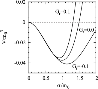
Figure 1: Behavior of the effective potential in Minkowski space-time for $G_{1}<0$, $G_{r}=-0.1,0,0.1$ and $D=3$.

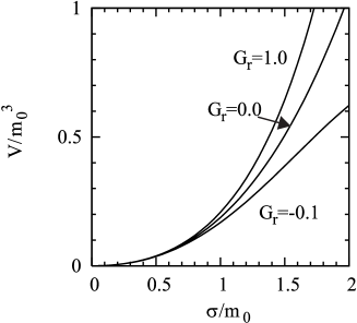
Figure 2: Behavior of the effective potential in Minkowski space-time for $G_{1}>0$, $G_{r}=-0.1,0,0.1$ and $D=3$.

Numerically evaluating the effective potential (28) as $G_{r}(\equiv G_{2}m_{0}^{2}/G_{1}^{3})$ varies, we find the phase structure. We set $D=3$ and show the typical behavior of the effective potential in Figs. 2 and 2 for a negative $G_{1}$ and a positive $G_{1}$, respectively. As is shown in Fig. 2, a positive eight-fermion coupling, $G_{2}$, enhances the chiral symmetry breaking, while a negative one suppresses it. For a positive $G_{1}$ we observe only the symmetric phase in Fig. 2. It should be noted that we can find a minimum of the effective potential, if we evaluate it for a larger $\sigma$. In the case of $G_{r}=-0.1$ with a positive $G_{1}$, we find a minimum at $\sigma/m_{0}\sim 3.8$. However, the expectation value of $\sigma$ is too large to keep validity of the model. It is outside the scope of our interest.

3 Curvature Induced Phase Transition

The space-time curvature may play an important role for a phase transition at the early universe. Here we evaluate the four- and eight-fermion interaction model (1) in a curved space-time. Some assumption for the back ground metric is necessary to calculate the ground state of the model. Here we assume that the space-time curves slowly and keep only terms independent of the curvature $R$ and terms linear in $R$.

For this purpose we introduce the Riemann normal coordinate system in which the affine connection vanishes at least locally[24]. Near the origin $x_{0}$ the back-ground metric is expanded to be

$$g_{\mu\nu}(x)=\eta_{\mu\nu}+\frac{1}{3}R_{\mu\alpha\nu\beta}(x-x_{0})^{\alpha}(x-x_{0})^{\beta}+O(R_{;\mu},R^{2}),$$ (32)

where $\eta_{\mu\nu}$ is the metric tensor on $R^{D}$, diag$(1,-1,\cdots,-1)$ and $R_{\mu\alpha\nu\beta}$ the curvature tensor at the origin. In the Riemann normal coordinate system the spinor two-point function (15) is found to be[5, 20]

$$S(x_{0},y;s) = \int\frac{d^{D}k}{(2\pi)^{D}}e^{-ik(x_{0}-y)}\left[\frac{\gamma^{a}k_{a}+s}{k^{2}-s^{2}}-\frac{1}{12}R\frac{\gamma^{a}k_{a}+s}{(k^{2}-s^{2})^{2}}\right.$$ (33)

$$\left.+\frac{2}{3}R^{\mu\nu}k_{\mu}k_{\nu}\frac{\gamma^{a}k_{a}+s}{(k^{2}-s^{2})^{3}}+\frac{1}{4}\gamma^{a}\sigma^{cd}R_{cda\mu}k^{\mu}\frac{1}{(k^{2}-s^{2})^{2}}\right]$$

$$+O(R_{;\mu},R^{2}).$$

Substituting Eq.(33) into Eq.(14), we expand the effective potential in terms of the space-time curvature $R$,

$$V(s,\sigma^{\prime})=V_{0}(s,\sigma^{\prime})-\frac{\mbox{tr1}}{(4\pi)^{D/2}}\frac{R}{24}\Gamma\left(1-\frac{D}{2}\right)|s|^{D-2}+O(R_{;\mu},R^{2}),$$ (34)

where $V_{0}(s,\sigma^{\prime})$ is the effective potential (27) for $R=0$. Since the term linear in $R$ is independent on $\sigma^{\prime}$, the stationary condition (17) is not modified. The auxiliary fields $s$ and $\sigma^{\prime}$ is rewritten by $\sigma$ by Eq.(19) with Eq.def:tsig at the stationary point. Thus the effective potential (34) reads

$$V(\sigma)=V_{0}(\sigma)-\frac{\mbox{tr1}}{(4\pi)^{D/2}}\frac{R}{24}\Gamma\left(1-\frac{D}{2}\right)\left|\sigma+\frac{G_{2}}{2G_{1}^{3}}\sigma^{3}\right|^{D-2}+O(R_{;\mu},R^{2}).$$ (35)

The gap equation defined by (20) reads

$$s = 2G_{1}\frac{\mbox{tr}1}{(4\pi)^{D/2}}\Gamma\left(1-\frac{D}{2}\right)s\left(|s|^{D-2}-\frac{D-2}{24}R|s|^{D-4}\right)$$ (36)

$$+4G_{2}\left[\frac{\mbox{tr}1}{(4\pi)^{D/2}}\Gamma\left(1-\frac{D}{2}\right)s\left(|s|^{D-2}-\frac{D-2}{24}R|s|^{D-4}\right)\right]^{3}.$$

It gives the necessary condition for the dynamically generated fermion mass in a weakly curved space-time. Evaluating the effective potential (35) and the gap equation (36) in weakly curved space-time, we study the curvature induce phase transition below.

3.1 Phase structure for a negative $G_{1}$

For a negative $G_{1}$ the chiral symmetry is broken in Mikowski space-time. We set $D=3$ and numerically draw the typical behavior of the effective potential for $G_{1}<0$ in Fig. 4. A positive $G_{r}$ suppresses the chiral symmetry breaking, while a negative one enhances it. The chiral symmetry is broken in Minkowski space-time for a negative $G_{1}$. The first order phase transition takes place, as the curvature increases. Thus the broken chiral symmetry is restored for a large positive $R$.

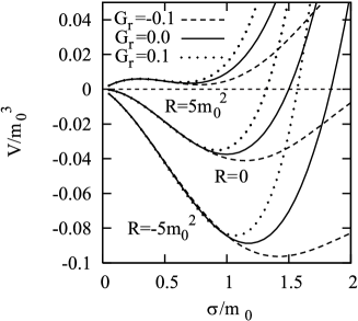
Figure 3: Behavior of the effective potential for $D=3$, $G_{1}<0$ and $G_{r}=-0.1,0,0.1$ as the curvature, $R$, varies.

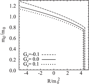
Figure 4: Dynamically generated fermion mass for $D=3$, $G_{1}<0$ and $G_{r}=-0.1,0,0.1$ as a function of $R$.

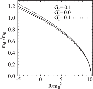
Figure 5: Dynamically generated fermion mass at the four-dimensional limit for $G_{1}<0$ and $G_{r}=-0.1,0,0.1$ as a function of $R$.

Figure 6: Phase structure as a function of the space-time dimension $D$ for $G_{1}<0$, $G_{r}=-0.1,0$ and $0.1$.

In Figs. 4 and 6 the dynamical fermion mass is plotted as a function of the space-time curvature, $R$. We numerically evaluate the true minimum of the effective potential, as the curvature $R$ varies, and obtain the solution corresponding to the true minimum. In Fig. 4 the mass gap appears at the critical point. Thus the phase transition is of the first order for $2\leq D<4$. A negative $G_{r}$ enhances the symmetry breaking and a larger critical curvature is observed for a negative $G_{r}$. We obtain a smaller $R_{cr}$ for a positive $G_{r}$.

Because of the non-renormalizability of the four- and the eight-fermion interactions, we can not remove all the divergence at the four dimensional limit. For example, the right-hand side in the gap equation (36) is divergent at the limit. If we normalize all the mass scales in the gap equation by $m_{0}$ given in Eq.(30), the factor $\Gamma({1-D/2})$ in $m_{0}$ eliminates the one in the gap equation. Thus we obtain a finite expression for the gap equation at the limit, $D\rightarrow 4$,

$$\frac{s}{m_{0}} = -\mbox{sgn}(G_{1})\frac{s}{m_{0}}\left[\left(\frac{s}{m_{0}}\right)^{2}-\frac{1}{12}\frac{R}{m_{0}^{2}}\right]$$ (37)

$$-\mbox{sgn}(G_{1})\frac{G_{r}}{2}\left(\frac{s}{m_{0}}\right)^{3}\left[\left(\frac{s}{m_{0}}\right)^{2}-\frac{1}{12}\frac{R}{m_{0}^{2}}\right]^{3}.$$

We plot the solution of Eq.(37) in Fig. 6 for a negative $G_{1}$. The broken chiral symmetry is restored through the second order phase transition at $R/m_{0}^{2}=12$. The critical value is independent on the eight-fermion coupling $G_{2}$. Therefore we obtain the critical curvature, $R_{cr}$, as a function of the space-time dimension, $D$. In Fig. 6 we illustrate the phase boundary which divides the symmetric phase and the broken phase for $G_{1}<0$ and $G_{r}=-0.1,0,0.1$. We find a positiveness of the critical curvature. Only the broken phase is realized in a space-time with a negative curvature.[8] The eight-fermion interaction contributes the curvature induced phase transition. Especially, we observe a endpoint, A, for $G_{r}=-0.1$.[25] At the point a the local minimum disappears from the range, $\langle\sigma\rangle/m_{0}\lesssim 1$, considered here.

3.2 Phase structure for a positive $G_{1}$

The chiral symmetry is preserved in Minkowski space-time for a positive $G_{1}$.

Figure 7: Behavior of the effective potential for $D=3$, $G_{1}>0$ and $G_{r}=-0.4,0,0.4$ as the curvature, $R$, varies.

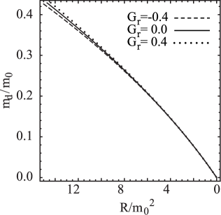
Figure 8: Dynamically generated fermion mass for $D=3$, $G_{1}>0$ and $G_{r}=-0.4,0,0.4$ as a function of $R$.

The space-time curvature modifies the effective potential, as is shown in Fig. 8. The effective potential has a single and a double well shape in a space-time with a non-negative and a negative curvature, respectively. An influence of the eight-fermion interaction is presented by dashed and dotted lines.

Though the eight-fermion interaction modifies the effective potential, it can not change the phase structure for a positive $G_{1}$. Such a situation can be clearly seen on the behavior of the dynamical fermion mass. We solve the gap equation (36) and draw the dynamical fermion mass as a function of the space-time curvature in Figs. 8 and 10. As is shown in Fig. 8, the dynamically generated fermion mass disappears at $R=0$ for $2\leq D<4$. Thus the critical curvature is given by $R_{cr}=0$ and the chiral symmetry is always broken for a negative $R$. Only the symmetric phase is realized for a non-negative $R$. In Figs. 10 and 10 we observe that the critical curvature shifts to a smaller value $R_{cr}/m_{0}^{2}=-12$ at the four-dimensional limit. Higher than the second order phase transition occurs at $R=0$ for $2\leq D<4$, while the second order phase transition takes place at $R/m_{0}^{2}=-12$ for $D\rightarrow 4$. As is discussed in the previous section, the critical value is independent of the eight-fermion coupling. Fig.10 shows the transition from $R_{cr}=0$ to $R_{cr}/m_{0}^{2}=-12$ for $G_{r}=0$, as the space-time dimension, $D$, varies.

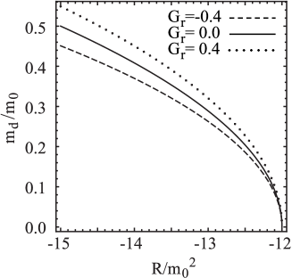
Figure 9: Dynamically generated fermion mass at the four-dimensional limit for $G_{1}>0$ and $G_{r}=-0.4,0,0.4$ as a function of $R$.

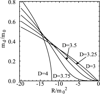
Figure 10: Dynamically generated fermion mass for $G_{1}>0$, $G_{r}=0$, $D=3,3.25,3.5,3.75$ and the limit $D\rightarrow 4$ as a function of $R$.

4 Finite Size and Topological Effects

The very early universe may have a non-trivial topology. A symmetry restoration at high temperature can be also classified as the similar type of effects. In this section we investigate the contribution from the eight-fermion interaction to the dynamical symmetry breaking in a flat space-time with non-trivial topology, $R^{D-1}\otimes S^{1}$.

In the compact manifold $S^{1}$ fermion fields should obey the boundary condition,

$$\psi(x+L)=e^{i\delta_{p,1}\pi}\psi(x),$$ (38)

where $L$ is the size of the $S^{1}$ direction. Since the boundary condition (38) restricts the allowed mode functions, the Fourier transformation in Eq. (26) is replaced by the Fourier series expansion,

$$\left\{\begin{array}[]{rcl}\displaystyle\int^{\infty}_{\infty}\frac{dk^{i}}{2\pi}&\rightarrow&\displaystyle\frac{1}{L}\sum_{n=-\infty}^{\infty},\\ k^{i}&\rightarrow&\displaystyle\frac{(2n+\delta_{p,1})\pi}{L},\end{array}\right.$$ (39)

where the upper index $i$ shows the compact direction, $S^{1}$, and $\delta_{p,1}$ is fixed by the boundary condition. Thus the spinor two point function (15) in $R^{D-1}\otimes S^{1}$ is found to be

$$S(x,y;s)=\frac{1}{L}\sum_{n=-\infty}^{\infty}\int\frac{d^{D-1}k}{(2\pi)^{D-1}}e^{-ik(x-y)}\frac{1}{\gamma^{\mu}k_{\mu}-s}.$$ (40)

Substituting Eq. (40) into Eq. (14), we obtain the effective potential in $R^{D-1}\otimes S^{1}$,

$$V(s,\sigma^{\prime}) = -\frac{\sigma^{\prime 2}}{4G_{1}}+\frac{s^{2}}{4G_{1}}-\frac{G_{2}}{16G_{1}^{4}}(\sigma^{\prime}+s)^{4}+\frac{\mbox{tr1}}{2(4\pi)^{(D-1)/2}}\Gamma\left(\frac{1-D}{2}\right)\frac{1}{L}$$ (41)

$$\times\sum_{n=-\infty}^{\infty}\left[\left(\frac{(2n+\delta_{p,1})\pi}{L}\right)^{2}+s^{2}\right]^{(D-1)/2}.$$

The stationary condition (17) is not modified. The auxiliary fields $s$ and $\sigma^{\prime}$ are represented by $\sigma$ at the stationary point. We insert Eq. (19) into Eq. (41) and rewrite the effective potential,

$$V(\sigma) = \frac{1}{4G_{1}}\left(\sigma^{2}+\frac{3G_{2}}{4G_{1}^{3}}\sigma^{4}\right)+\frac{\mbox{tr1}}{2(4\pi)^{(D-1)/2}}\Gamma\left(\frac{1-D}{2}\right)\frac{1}{L}$$ (42)

$$\times\sum_{n=-\infty}^{\infty}\left[\left(\frac{(2n+\delta_{p,1})\pi}{L}\right)^{2}+\left(\sigma+\frac{G_{2}}{2G_{1}^{3}}\sigma^{3}\right)^{2}\right]^{(D-1)/2}.$$

The necessary condition for the dynamical fermion mass is given by the gap equation defined by (20). We substitute the two-point function (40) into Eq. (20) and obtain

$$s = 2G_{1}\frac{\mbox{tr}1}{(4\pi)^{(D-1)/2}}\Gamma\left(\frac{1-D}{2}\right)\frac{s}{L}\sum_{n=-\infty}^{\infty}\left[\left(\frac{(2n+\delta_{p,1})\pi}{L}\right)^{2}+s^{2}\right]^{(D-3)/2}$$ (43)

$$+4G_{2}\Biggl{\{}\frac{\mbox{tr}1}{(4\pi)^{(D-1)/2}}\Gamma\left(\frac{1-D}{2}\right)\frac{s}{L}$$

$$\times\sum_{n=-\infty}^{\infty}\left[\left(\frac{(2n+\delta_{p,1})\pi}{L}\right)^{2}+s^{2}\right]^{(D-3)/2}\Biggl{\}}^{3}.$$

Below we evaluate the effective potential (42) and the gap equation (43) for fermions with the periodic, $\delta_{p,1}=0$, and the anti-periodic boundary conditions, $\delta_{p,1}=1$ and discuss the phase structure.

4.1 Phase structure for a negative $G_{1}$

In Minkowski space-time, $R^{D}$, the system is in the broken phase for a negative $G_{1}$. The space-time, $R^{D}$, is obtained at the large $L$ limit, $L\rightarrow\infty$, of $R^{D-1}\otimes S^{1}$. We start from the broken phase at the large $L$ limit and evaluate the effective potential as $L$ decreases.

Figure 11: Behavior of the effective potential for $D=3$, $G_{1}<0$ and $G_{r}=-0.1,0,0.1$ in the case of the anti-periodic boundary condition.

Figure 12: Dynamical fermion mass for $D=3$, $G_{1}<0$ and $G_{r}=-0.1,0,0.1$ as a function of the length $L$ in the case of the anti-periodic boundary condition.

In the case of the anti-periodic boundary condition the theory on $R^{D-1}\otimes S^{1}$ is equivalent to the finite temperature theory. It is expected that a broken symmetry is restored at high temperature. Thus the finite size effect should also restore the broken symmetry. We draw the typical behavior of the effective potential (42) for the fermion field with the anti-periodic boundary condition in Fig. 12. The broken chiral symmetry is restored for a small $L$.

The dynamically generated mass for the fermion field with the anti-periodic boundary condition is plotted in Fig. 12 by solving the gap equation (43). It is clearly seen that the dynamical fermion mass disappears and the broken chiral symmetry is restored through the second order phase transition at the critical length, $L_{cr}$. The dynamical fermion mass is modified by the eight-fermion interaction. As is discussed in Sec. 2, the eight-fermion interaction does not affect the critical length, $L_{cr}$. We can analytically calculate the critical length, $L_{cr}$, by taking the limit $s\rightarrow 0$ for the non-trivial solution of the gap equation (43). Thus we find the explicit expression for the critical length, $L_{cr}$,

$$L_{cr}=2\pi\left[\frac{2\mbox{tr1}G_{1}}{\pi(4\pi)^{(D-1)/2}}(2^{3-D}-1)\Gamma\left(\frac{3-D}{2}\right)\zeta(3-D)\right]^{1/(D-2)}.$$ (44)

for fermion fields with the anti-periodic boundary condition. We plot it as a function of the space-time dimension, $D$, in Fig. 14. Though the effective potential (28) is divergent at the four-dimensional limit, the finite size effect gives a finite correction for the divergent potential. The effect disappears at the four-dimensional limit.

Figure 13: Phase diagram for $G_{1}<0$ in the case of the anti-periodic boundary condition.

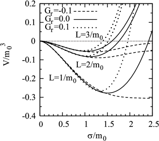
Figure 14: Behavior of the effective potential for $D=3$, $G_{1}<0$ and $G_{r}=-0.1,0,0.1$ in the case of the periodic boundary condition.

We draw the behavior of the effective potential for the fermion field with the periodic boundary condition in Fig. 14. The finite size effect enhances the chiral symmetry breaking in this case. Thus only the broken phase can be realised for a negative $G_{1}$. If we enlarge the scope of our analysis to include a larger $\sigma$, the eight-fermion interaction induces another type of transition between finite $\sigma$. As is shown in Fig. 16, the effective potential can develop two local minima for $G_{r}=-0.1$. The finite size effect shifts the true minimum from the first to the second local one which is outside the scope of our interest. In Fig. 16 we plot the dynamical fermion mass in the case of the periodic boundary condition by solving the gap equation (43). The finite size effect increases the dynamically generated fermion mass. For a negative $G_{r}$ we observe a small mass gap which is induced by the transition from the first to the second minimum in Fig. 15. Then the two minima combined at $\sigma/m_{0}=\sqrt{-2/(3G_{r})}$, as $L$ deceases. If the size $L$ is small enough, the dynamical fermion mass is given by

$$m_{d}/m_{0}=\sqrt{-\frac{2}{3G_{r}}}+\frac{G_{r}}{2}\left(-\frac{2}{3G_{r}}\right)^{3/2},$$ (45)

for a negative $G_{r}$.

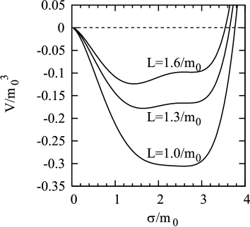
Figure 15: Behavior of the effective potential for $D=3$, $G_{1}<0$ and $G_{r}=-0.1$ in the case of the periodic boundary condition.

Figure 16: Dynamical fermion mass for $D=3$, $G_{1}<0$ and $G_{r}=-0.1,0,0.1$ as a function of the length $L$ in the case of the periodic boundary condition.

4.2 Phase structure for a positive $G_{1}$

For a positive $G_{1}$ the system is in the symmetric phase at the Minkowski limit, $L\rightarrow\infty$. To study the chiral symmetry breaking induced by the finite size effect we evaluate the effective potential (42). In the case of the anti-periodic boundary condition the finite size effect works to stabilize the trivial ground state at $\sigma=0$. Thus only the symmetric phase can be realized. We can not observe any transition of the ground state. Therefore it is enough to analyze only fermion fields which obey the periodic boundary condition.

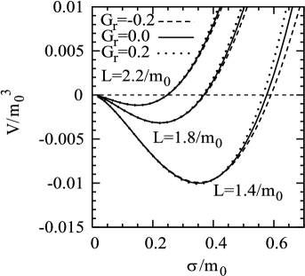
Figure 17: Behavior of the effective potential for $D=3$, $G_{1}>0$ and $G_{r}=-0.2,0,0.2$ in the case of the periodic boundary condition.

Figure 18: Dynamical fermion mass for $D=3$, $G_{1}>0$ and $G_{r}=-0.2,0,0.2$ as a function of the length $L$ in the case of the periodic boundary condition.

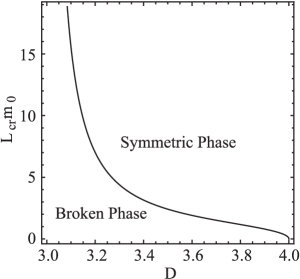
Figure 19: Phase diagram for $G_{1}>0$ in the case of the periodic boundary condition.

For fermion fields with the periodic boundary condition we plot the behavior of the effective potential in Fig. 18. The effective potential has the double well shape for a small $L$. Thus the phase transition is caused by the finite size effect. The order of the transition is found by observing the dynamical fermion mass. We draw it as a function of $L$ in Fig. 18. It is found that the phase transition is of higher than the second order. The eight-fermion interaction has larger contribution for a negative $G_{r}$. In this case the dynamical fermion mass is give by Eq.(45) again, if $L$ is small enough.

The critical length, $L_{cr}$, is derived by taking the limit $s\rightarrow 0$ for the non-trivial solution of the gap equation (43). It is found to be

$$L_{cr}=2\pi\left[\frac{2\mbox{tr1}G_{1}}{\pi(4\pi)^{(D-1)/2}}\Gamma\left(\frac{3-D}{2}\right)\zeta(3-D)\right]^{1/(D-2)},$$ (46)

for fermion fields with the periodic boundary condition. The chiral symmetry is broken at $L=L_{cr}$. We illustrate the phase diagram for $G_{1}>0$ in the case of the periodic boundary condition in Fig. 19. The eight-fermion interaction has nothing to do with the phase boundary. It should be noted that the finite size effect disappears at the four-dimensional limit.

5 Conclusion

In this article the four- and eight-fermion interaction model has been investigated in the two types of space-time, a weakly curved space-time and a cylindrical space-time, $R^{D-1}\otimes S^{1}$. The expectation value for the composite operator, $\bar{\psi}\psi$ is one of the order parameters for the chiral symmetry breaking. Thus the phase structure of the system is found by observing the effective potential in terms of the order parameter, $\sigma(\propto\bar{\psi}\psi)$. We have applied the dimensional regularization and have calculated the effective potential in the leading order of the $1/N$ expansion. The effective potential is written as a function of the auxiliary field, $\sigma$, space-time dimension, $D$, a ration of the coupling constant, $G_{r}=G_{2}/G_{1}^{3}$, and the sign of the four-fermion coupling, sgn$(G_{1})$. It has been shown that the stability of the critical point against the eight-fermion interaction. The eight-fermion interaction can not modify the phase boundary, if the phase transition is of the second or higher than second order.

In Minkowski space-time, $R^{D}$, the chiral symmetry is broken for a negative four-fermion coupling. As is mentioned in Ref. [35], the renormalized coupling can be positive. The eight-fermion interaction modifies the shape of the effective potential. Contributions from the eight-fermion interaction is enhanced for a larger $\sigma(\propto\bar{\psi}\psi)$. However, if the auxiliary field $\sigma$ develops a large value, we can not neglect higher dimensional operators which are not employed. We have analysed the system in the restricted parameter range, $\langle\sigma\rangle/m_{0}\lesssim 1$.

To study the curvature effect we have evaluated the effective potential in weakly curved space-time. In the four-fermion interaction model the broken symmetry is restored for a large positive curvature, $R$. The phase transition is of the first order for a negative four-fermion coupling, $G_{1}$ at $2\leq D<4$. Only the broken phase appears in a space-time with a negative curvature. The dynamically generated fermion mass is modified by the eight-fermion interaction. Except for the four-dimensional limit we have observed a lower and a higher critical curvature for a positive and a negative $G_{r}$, respectively. The phase boundary is shown as a function of $D$. If we consider a negative $G_{2}$, the minimum of the effective potential disappears inside the range, $\langle\sigma\rangle/m_{0}\lesssim 1$. The phase boundary vanishes at a low dimension for $G_{2}<0$. In Ref. [30] the cutoff regularization is applied to analyse the same model in weakly curved space-time at $D=4$. Since the four- and eight-fermion interaction are non-renormalizable in four dimensions, the phase structure depends on the regularization procedures.

The space-time topology also has non-negligible contribution for the expectation value of the composite operator, $\bar{\psi}\psi$. We have investigated the flat space-time with nontrivial topology, $R^{D-1}\otimes S^{-1}$ and found the phase structure of the system. The finite size effect can induce the second or higher than second order phase transition. Thus the critical length does not modified by the eight-fermion interaction. We have obtained the phase boundary independent of the eight-fermion coupling, $G_{2}$. The system for fermion fields with the anti-periodic boundary condition is equivalent to the finite temperature field theory in Matsubara Formalism. There is a correspondence between the phase boundary in Fig. 14 and the one at finite temperature, $T$, if we make a replacement,

$$L\leftrightarrow\frac{1}{k_{B}T},$$ (47)

For a negative $G_{r}$ and $G_{1}$ two local minima are observed in the effective potential, though the second one is outside the range, $\langle\sigma\rangle/m_{0}\lesssim 1$.

In the present paper we have studied a simple toy model of the dynamical symmetry breaking. But we believe that the curvature and the topological effects on the dynamical symmetry breaking is similar in general to the case we have investigated. To distinguish a characteristic feature of the model we will continue our works in other models, vector-type fermion interactions, gauge theories and the supersymmetric extension of the model and so on in various background space-time. Here we focus on the mathematical aspects of the four- and eight-fermion interaction model. However, we are interested in the application of our analysis to phenomena at the early universe. It is expected that the spontaneous symmetry breaking has play an essential role for the evolution of the space-time. To study the evolution of the universe we should calculate the stress tensor and solve the Einstein equation. We will continue our works and hope to report on these problems.

References

- [1] Y. Nambu and G. Jona-Lasinio, Phys. Rev. 124, 246 (1961).
- [2] D. J. Gross and A. Neveu, Phys. Rev. D 10, 3235 (1974).
- [3] H. Itoyama, Prog. Theor. Phys. 64, 1886 (1980).
- [4] I. L. Buchbinder and E. N. Kirillova, Int. J. of Mod. Phys. A 4, 143 (1989).
- [5] T. Inagaki, T. Muta and S. D. Odintsov, Mod. Phys. Lett. A 8, 2117 (1993).
- [6] E. Elizalde, S. D. Odintsov and Yu. I. Shil’nov, Mod. Phys. Lett. A 9, 913 (1994).
- [7] T. Inagaki, Int. J. of Mod. Phys. A 11, 4561 (1996).
- [8] E. V. Gorbar, Phys. Rev. D 61, 024013 (2000).
- [9] A. S. Vshivtsev, K. G. Klimenko and B. V. Magnitsky, Phys. Atom. Nucl. 59, 529 (1996). [Yad. Fiz. 59, 557 (1996)].
- [10] S. K. Kim, W. Namgung, K. S. Soh and J. H. Yee, Phys. Rev. D 36, 3172 (1987).
- [11] D. Y. Song and J. K. Kim, Phys. Rev. D 41, 3165 (1990).
- [12] D. K. Kim, Y. D. Han and I. G. Koh, Phys. Rev. D 49, 6943 (1994).
- [13] K. Ishikawa, T. Inagaki, K. Yamamoto and K. Fukazawa, Prog. Theor. Phys. 99, 237 (1998).
- [14] L. M. Abreu, M. Gomes and A. J. da Silva, Phys. Lett. B 642, 551 (2006).
- [15] T. Inagaki, S. Mukaigawa and T. Muta, Phys. Rev. D 52, 4267 (1995).
- [16] E. Elizalde, S. Leseduarte, S. D. Odintsov and Yu. I. Shilnov, Phys. Rev. D 53, 1917 (1996).
- [17] K. Ishikawa, T. Inagaki and T. Muta, Mod. Phys. Lett. A 11, 939 (1996).
- [18] E. Elizalde, S. Leseduarte and S. D. Odintsov, Phys. Rev. D 49, 5551 (1994).
- [19] D. Ebert, K. G. Klimenko, A. V. Tyukov and V. C. Zhukovsky, Eur. Phys. J. C 58, 57 (2008).
- [20] T. Inagaki, T. Muta and S. D. Odintsov, Prog. Theor. Phys. Suppl. 127, 93 (1997).
- [21] G. ’t Hooft, Phys. Rev. D 14, 3432 (1976); Phys. Rev. D 18, 2199 (1978) (E); Phys. Rep. 142, 357 (1986).
- [22] R. Alkofer and I. Zahed, Phys. Lett. B 238, 149 (1990).
- [23] E. Elizalde, S. Leseduarte and S. D. Odintsov, Phys. Lett. B 347, 33 (1995).
- [24] A. Z. Petrov, Einstein Spaces, (Pergamon, Oxford, 1969).
- [25] T. Inagaki and M. Hayashi, Topological and curvature effects in a multi-fermion interaction model, arXiv:1003.1173 [hep-ph]
- [26] A. A. Osipov, B. Hiller, A. H. Blin and J. da Providencia, Ann. Phys. 322, 2021-2054 (2007).
- [27] E. Elizalde and S. D. Odintsov, Mod. Phys. Lett. A 10, 733 (1995).
- [28] E. Elizalde and S. D. Odintsov, Phys. Rev. D 51, 5950 (1995).
- [29] I. L. Buchbinder, T. Inagaki and S. D. Odintsov, Mod. Phys. Lett. A 12, 2271 (1997).
- [30] M. Hayashi, T. Inagaki and H. Takata, Int. J. Mod. Phys. A 24, 5363 (2009).
- [31] S. Krewald and K. Nakayama, Ann. Phys. 216, 201 (1992).
- [32] H.-J. He, Y.-P. Kuang, Q. Wang and Y.-P. Yi, Phys. Rev. D 45, 4610 (1992).
- [33] T. Inagaki, T. Kouno and T. Muta, Int. J. Mod. Phys. A 10, 2241 (1995).
- [34] R. G. Jafarov and V. E. Rochev, Russ. Phys. J. 49, 364 (2006).
- [35] T. Inagaki, D. Kimura and A. Kvinikhidze, Phys. Rev. D 77, 116004 (2008); T. Fujihara, D. Kimura, T. Inagaki and A. Kvinikhidze, Phys. Rev. D 79, 096008 (2009).