Smooth cosmological phase transition in the Hořava-Lifshitz gravity

Abstract

We show that the cosmological phase transition from the first accelerated expansion in the early universe to the second accelerated expansion over the intermediate decelerated expansion is possible in the HL gravity without the “detailed balance” condition if the dark scalar energy density is assumed to be negative. Moreover, we obtain various evolutions depending on the scale factor and the expansion rate. Finally, we discuss the existence of the minimum scale in connection with the singularity free condition.

I Introduction

Recently, the Hořava-Lifshitz (HL) gravity has been proposed as an ultraviolet (UV) completion of general relativity horava , motivated by the Lifshitz theory in the condensed matter physics lifshitz . The key of the UV completion is the anisotropic scaling between space and time,

$$t\to b^{z}\,t,\qquad x^{i}\to b\,x^{i},$$ (1)

where the Lifshitz parameter $z$ becomes 1 in the infrared (IR) limit. In general, the HL theory is not invariant under the full diffeomorphism group of general relativity but under its subgroup, called the foliation-preserving diffeomorphism; however, in the IR limit, the full diffeomorphism is somehow recovered. A mechanism for recovering the full diffeomorphism or the renormalization group flow is yet unsolved issue, but the HL gravity has been intensively studied in the area of cosmology ts ; kk ; mukohyama ; brandenberger ; ks ; ww ; mipark ; ls ; sj and black hole physics lmp ; cco ; cy ; ysmyung ; mann ; gh ; kk:bh ; majhi .

Considering Arnowitt-Deser-Misner (ADM) decomposition  of the metric with $ds^{2}=-N^{2}c^{2}dt^{2}+g_{ij}(dx^{i}+N^{i}dt)(dx^{j}+N^{j}dt)$ adm , the Einstein-Hilbert action can be rewritten as

$$I_{EH} =\frac{c^{3}}{16\pi G_{N}}\int d^{4}x\sqrt{-\mathcal{G}}\left[\mathcal{R}-2\Lambda\right]$$ (2)

$$=\frac{c^{2}}{16\pi G_{N}}\int dtd^{3}x\sqrt{g}N\left[K_{ij}K^{ij}-K^{2}+c^{2}\left(R-2\Lambda\right)\right],$$

where $K_{ij}\equiv\frac{1}{2N}\left[\dot{g}_{ij}-\nabla_{i}N_{j}-\nabla_{j}N_{i}\right]$ is the extrinsic curvature of $t=\text{constant}$ hyper-surface, and the dot denotes the derivative with respect to $t$. Here, $g_{ij}$, $R$, and $\nabla_{i}$ are the metric, the intrinsic curvature, and the covariant derivative in the three-dimensional hyper-surface, respectively. Note that the action (2) can be regarded as one of the $z=1$ HL theory and each terms are invariant under the foliation-preserving diffeomorphism. Then, the first two terms are referred to as kinetic terms, while the other two are potential terms.

In particular, to study the HL gravity, higher-order potential terms, for instance, $R^{3}$, will be taken into account. But there are almost ten possible terms for $z=3$ case, and the “detailed balance” condition can reduce the ten coefficients to three effective ones horava . Of course, it also implies that $(D+1)$-dimensional renormalization can be reduced to the simpler $D$-dimensional renormalization. By the way, it has been claimed that matter is not UV stable with this condition calcagni , and the HL theory with the detailed balance condition does not have the Minkowski vacuum solution.

On the other hand, there have been interesting studies on the cosmological evolution in the HL gravity based on the phase space analysis ls . Authors showed that the cosmological phase changing from the decelerated expansion to the accelerated expansion is possible assuming the detailed balance condition and the constant equation-of-state parameter. However, the first accelerated expansion corresponding to the inflationary era has not been discussed. We believe that there should be such a structure if the HL theory is indeed the UV completion. By the way, the HL gravity itself may be problematic, for instance, counting its degrees of freedom lp ; hkg , description of the asymptotically flat spacetime ks ; lmp , and so on. However, even in spite of these problems, it deserves to study various aspects since it may give some insight to understand the quantum gravity. So, we would like to investigate whether the smooth cosmological phase transition from the first accelerated expansion in the early universe to the second accelerated expansion over the intermediate decelerated expansion is possible or not.

In section II, we recapitulate the Hořava-Lifshitz cosmology and define some relevant quantities without the “detailed balance” condition. Then, the nonlinear equations of motion will be solved using nonlinear methods in order to study the cosmological behavior in section III. By considering the observational data on density parameters, we shall plot the phase portrait in section IV, and discuss the behavior in the early stage of our universe and its various destiny. If a dark scalar energy density is assumed to be negative, then the desired first accelerated expansion appears. Moreover, we will show that it can be smoothly connected with the second accelerated expansion. Finally, discussions will be given in section V.

II Cosmological setting for $z=3$

We now consider the anisotropic scaling (1) between time and space, and then $g_{ij}$ and $N$ are invariant while $N^{i}\to b^{1-z}N^{i}$ and $c\to b^{1-z}c$. Requiring that the Planck constant is also invariant, $\hbar\to\hbar$, we get $E\to b^{-z}E$ and $M\to b^{z-2}M$, where $E$ and $M$ are energy and mass, respectively. Then, the kinetic action in the Hořava-Lifshitz gravity (HL) is naturally given as

$$I_{\text{kin}}=\frac{2}{\kappa^{2}}\int dtd^{3}x\sqrt{g}N\left[K_{ij}K^{ij}-\lambda K^{2}\right],$$ (3)

where $\kappa^{2}$ is a coupling related to the Newton constant $G_{N}$, and $\lambda$ is an additional dimensionless coupling constant. Note that the original kinetic part of Einstein-Hilbert action (2) can be recovered when $\lambda=1$ and $\kappa^{2}=32\pi G_{N}/c^{2}$. Moreover, the power-counting renormalizability requires $z\geq 3$ horava . From now on, we will choose $z=3$ for simplicity, then $\kappa^{2}$ becomes dimensionless because of $\kappa^{2}\to b^{3-z}\kappa^{2}$.

Now, the most general potential for $z=3$ can be written as

$$I_{\text{pot}}=-\frac{2}{\kappa^{2}}\int dtd^{3}x\sqrt{g}N\Big{[}\alpha+\beta R+\gamma_{1}R^{2}+\gamma_{2}R_{ij}R^{ij}+\xi\varepsilon^{ijk}R_{i\ell}\nabla_{j}R_{k}^{\ell}$$ (4)

$$+\sigma_{1}R^{3}+\sigma_{2}RR_{ij}R^{ij}+\sigma_{3}R_{i}^{j}R_{j}^{k}R_{k}^{i}+\sigma_{4}\nabla_{i}R\nabla^{i}R+\sigma_{5}\nabla_{i}R_{jk}\nabla^{i}R^{jk}\Big{]}.$$

Note that other possible terms are not independent because of the Bianchi identity and symmetries of Riemann tensors. The potential terms in Eq. (2) can be recovered when we set $\alpha=2\Lambda c^{2}$, $\beta=-c^{2}$, and $\gamma_{i}=\xi=\sigma_{i}=0$. Then, the fundamental constants can be identified with

$$c=\sqrt{-\beta},\qquad G_{N}=\frac{\kappa^{2}c^{2}}{32\pi},\qquad\Lambda=-\frac{\alpha}{2\beta}.$$ (5)

On the other hand, the ten coefficients can be reduced to three, $\mu$, $\Lambda_{W}$, $\zeta$, using the detailed balance condition horava :

$$\alpha=-\frac{3\kappa^{4}\mu^{2}\Lambda_{W}^{2}}{16(3\lambda-1)},\ \beta=\frac{\kappa^{4}\mu^{2}\Lambda_{W}}{16(3\lambda-1)},\ \gamma_{1}=\frac{\kappa^{4}\mu^{2}(1-4\lambda)}{64(3\lambda-1)},\ \gamma_{2}=\frac{\kappa^{4}\mu^{2}}{16},\ \xi=-\frac{\kappa^{4}\mu}{4\zeta^{2}},$$ (6)

$$\sigma_{1}=\frac{\kappa^{4}}{8\zeta^{4}},\ \sigma_{2}=-\frac{5\kappa^{4}}{8\zeta^{4}},\ \sigma_{3}=\frac{3\kappa^{4}}{4\zeta^{4}},\ \sigma_{4}=-\frac{3\kappa^{4}}{32\zeta^{4}},\ \sigma_{5}=\frac{\kappa^{4}}{4\zeta^{4}},$$

for which the three-dimensional topologically massive gravity action djt is given by

$$W=\mu\int d^{3}x\sqrt{g}(R-2\Lambda_{W})+\frac{1}{\zeta^{2}}\int\chi(\Gamma),$$ (7)

where $\chi(\Gamma)$ represents the gravitational Chern-Simons term. However, we will take the general ten coefficients without resort to the detailed balance condition (6) so that the total action becomes

$$I=I_{\text{kin}}+I_{\text{pot}}+I_{\text{mat}}$$ (8)

where we introduced a normal matter action $I_{\text{mat}}$ which is a perfect fluid source of the energy density $\rho$ and the pressure $p$.

Now, we are going to consider the Robertson-Walker (RW) metric,

$$ds^{2}=-c^{2}dt^{2}+a^{2}(t)\left[\frac{dr^{2}}{1-kr^{2}}+r^{2}d\Omega_{2}^{2}\right],$$ (9)

where $k=0,\pm 1$ is the normalized spatial curvature. After some tedious calculations in Eqs. (8), the equations of motion can be obtained as

$$3(3\lambda-1)H^{2}= \ \frac{\kappa^{2}}{2}\rho+6\left[\frac{\alpha}{6}+\frac{k\beta}{a^{2}}+\frac{2k^{2}(3\gamma_{1}+\gamma_{2})}{a^{4}}+\frac{4k^{3}(9\sigma_{1}+3\sigma_{2}+\sigma_{3})}{a^{6}}\right],$$

$$= \ \frac{\kappa^{2}}{2}\left[\rho+\rho_{\text{vac}}+\rho_{k}+\rho_{\text{dr}}+\rho_{\text{ds}}\right],$$ (10)

$$(3\lambda-1)\left(\dot{H}+\frac{3}{2}H^{2}\right)= \ -\frac{\kappa^{2}}{4}p-3\left[-\frac{\alpha}{6}-\frac{k\beta}{3a^{2}}+\frac{2k^{2}(3\gamma_{1}+\gamma_{2})}{3a^{4}}+\frac{4k^{3}(9\sigma_{1}+3\sigma_{2}+\sigma_{3})}{a^{6}}\right],$$

$$= \ -\frac{\kappa^{2}}{4}\left[p+p_{\text{vac}}+p_{k}+p_{\text{dr}}+p_{\text{ds}}\right],$$ (11)

where $H=\dot{a}/a$ is the Hubble parameter. Apart from the normal matter contribution, the additional energy-momentum contributions from the potential terms (4) are explicitly written as

$$p_{\text{vac}}=-\rho_{\text{vac}}=-\frac{3c^{2}}{8\pi G_{N}}\frac{\alpha}{6}, p_{k}=-\frac{1}{3}\rho_{k}=-\frac{c^{2}}{8\pi G_{N}}\frac{k\beta}{a^{2}},$$ (12)

$$p_{\text{dr}}=\frac{1}{3}\rho_{\text{dr}}=\frac{c^{2}}{8\pi G_{N}}\frac{2k^{2}(3\gamma_{1}+\gamma_{2})}{a^{4}}, p_{\text{ds}}=\rho_{\text{ds}}=\frac{3c^{2}}{8\pi G_{N}}\frac{4k^{3}(9\sigma_{1}+3\sigma_{2}+\sigma_{3})}{a^{6}}.$$

Similarly to the general relativity, $\rho_{\text{vac}}$ and $\rho_{k}$ come from the vacuum energy and the spatial curvature contributions, respectively. In particular, in the HL theory, $\rho_{\text{dr}}$ is called the dark radiation. Moreover, $\rho_{\text{ds}}$ is a dark scalar, since it is characterized by $\rho_{\text{ds}}=p_{\text{ds}}\sim a^{-6}$. It is interesting to note that for the spatial flat geometry, the equations of motion (10) and (11) are reduced to those of general relativity up to a factor $(3\lambda-1)/2$; in other words, the given HL cosmology is prominent for the nonvanishing spatial curvature. Both $\rho_{\text{dr}}$ and $\rho_{\text{ds}}$ depend on the spatial curvature $k$; in this sense, these might be regarded as corrections to the curvature contribution $\rho_{k}$. The total actual energy can be defined by $\rho_{\text{tot}}=\rho+\rho_{\text{vac}}+\rho_{\text{dr}}+\rho_{\text{ds}}$.

From Eqs. (10) and (11), we can get the acceleration of the scale factor,

$$(3\lambda-1)\frac{\ddot{a}}{a}=-\frac{\kappa^{2}}{12}\left[\rho_{\text{tot}}+3p_{\text{tot}}\right],$$ (13)

where we used the relation $\rho_{k}+3p_{k}=0$. Next, differentiating Eq. (10) with respect to $t$ and plugging it into Eq. (11), we can naturally obtain the fluid equation $\dot{\rho}_{c}+3H\left(\rho_{c}+p_{c}\right)=0$, where $\rho_{c}$ is defined by $\rho_{c}\equiv 6(3\lambda-1)H^{2}/\kappa^{2}=\rho_{\text{tot}}+\rho_{k}$. Without loss of generality, the conservation equation becomes

$$\dot{\rho}_{i}+3H\left(\rho_{i}+p_{i}\right)=0,$$ (14)

which is valid for each source component, i.e., $\{\rho_{i}\}=\{\rho,\rho_{\text{vac}},\rho_{k},\rho_{\text{dr}},\rho_{\text{ds}}\}$.

III Linear analyses

Ultimately, we want to show the cosmological phase transition from the first accelerated expansion to the second accelerated expansion in terms of the intermediate decelerated expansion, which looks like the overall behavior of our universe. Before we get down to this problem, we are going to exhibit the essence of the linear analysis. First, rewriting Eq. (13), we have

$$(3\lambda-1)\frac{\ddot{a}}{a}=-\frac{\kappa^{2}}{12}[1+3\omega(a)]\rho_{\text{tot}},$$ (15)

where $\omega(a)=p_{\text{tot}}/\rho_{\text{tot}}$ is the equation-of-state parameter for the total energy. To describe phase portraits, we should make change of variables so that we introduce $v=\dot{a}$, and $h=\kappa^{2}\rho_{\text{tot}}/6(3\lambda-1)$ with $\lambda>1/3$. Then, we can get three first-order differential equations,

$$\dot{a}=v,$$ (16)

$$\dot{v}=-\frac{1}{2}\left[1+3\omega(a)\right]ah,$$

$$\dot{h}=-3\left[1+\omega(a)\right]\frac{vh}{a},$$

where we used Eqs. (14) and (15). Note that integrating Eq. (16), we can find a conservation relation,

$$a^{2}h-v^{2}=-\frac{2k\beta}{3\lambda-1},$$ (17)

where the integration constant in the right hand side of (17) was consistently fixed by comparing Eq. (10). Now, let us eliminate $h$ in Eq. (16) using the conservation relation (17), then we have just two first-order differential equations,

$$\dot{a}=v\equiv f(a,v),$$ (18)

$$\dot{v}=-\frac{1}{2a}\left[1+3\omega(a)\right]\left(v^{2}-\frac{2k\beta}{3\lambda-1}\right)\equiv g(a,v),$$ (19)

where the equation-of-state parameter can be written as $\omega(a)=-1-ah^{\prime}/3h$ with $h^{\prime}=dh/da$.

To study the behavior of the scale factor in the phase space, we should calculate the Jacobian matrix,

$$A=\left[\begin{array}[]{cc}\partial_{a}f&\partial_{v}f\\ \partial_{a}g&\partial_{v}g\end{array}\right]_{(a^{*},v^{*})}=\left[\begin{array}[]{cc}0&1\\ 3k\beta\omega^{\prime}(a^{*})/(3\lambda-1)a^{*}&0\end{array}\right],$$ (20)

on the fixed point $(a^{*},v^{*})$ which is easily obtained from $\dot{a}=\dot{v}=0$ in Eqs. (18) and (19),

$$(a^{*},v^{*})\text{ satisfying }\left\{\begin{aligned} &v^{*}=0,&&\text{for }k=0,\\ &1+3\omega(a^{*})=0,v^{*}=0,&&\text{for }k\neq 0.\end{aligned}\right.$$ (21)

Note that for $k=0$, there are non-isolated fixed points; i.e. every point on the line $v^{*}=0$ can be a fixed point. Next, considering an eigenvalue equation of $A\mathbf{V}=\eta\mathbf{V}$ which gives two eigenvalues, the fixed points can be classified as follows strogatz : They are repellers if both eigenvalues have positive real part, attractors if both eigenvalues have negative real part. In particular, they become saddles if one eigenvalue is positive and the other is negative. On the other hand, if both eigenvalues are pure imaginary, then they are centers. Moreover, they are called non-isolated fixed points if at least one eigenvalue is zero.

Specifically, the Jacobian matrix (20) for $k=0$, is trivial so that we can find non-isolated fixed points as mentioned earlier, due to the fact that at least one eigenvalue is zero. As for $k\neq 0$, the Jacobian matrix (20) becomes $A=\left[\begin{array}[]{cc}0&1\\ 3k\beta\omega^{\prime}(a^{*})/(3\lambda-1)a^{*}&0\end{array}\right]$, and the corresponding eigenvalues are $\eta=\pm\sqrt{3k\beta\omega^{\prime}(a^{*})/(3\lambda-1)a^{*}}$ where $\lambda>1/3$ is already assumed. Then, the fixed point (21) becomes a saddle node for $k\beta\omega^{\prime}(a^{*})>0$ or a center for $k\beta\omega^{\prime}(a^{*})<0$.

IV Cosmological phase transition

We are now in a position to specify the matter source which consists of the conventional cold matter and radiation, $\rho=\rho_{m}+\rho_{r}$ with $\rho_{m}\sim a^{-3}$ and $\rho_{r}\sim a^{-4}$. Let us define $\rho_{\text{rad}}=\rho_{r}+\rho_{\text{dr}}$, following the conventional way that $\rho_{m}$ means the density for the cold dark matter as well as baryons. Then, the equation-of-state parameter $\omega(a)$ is given by

$$\omega(a)=\frac{3\Omega_{\text{ds}}+a^{2}\Omega_{\text{rad}}-3a^{6}\Omega_{\text{vac}}}{3\left[\Omega_{\text{ds}}+a^{2}\Omega_{\text{rad}}+a^{3}\Omega_{m}+a^{6}\Omega_{\text{vac}}\right]},$$ (22)

where the density parameters are defined as $\Omega_{i}=\rho_{i}/\rho_{c}$ evaluated at the present universe scale $a_{0}$, which can be fixed to $a_{0}=1$. Note that the equation-of-state parameter becomes $\omega(a_{0})\simeq-\Omega_{\text{vac}}\simeq-0.7$ at the present scale, since the observational data indicates $\Omega_{\text{ds}},\Omega_{\text{rad}}\ll\Omega_{\text{vac}}\simeq 0.7$ wmap5 .

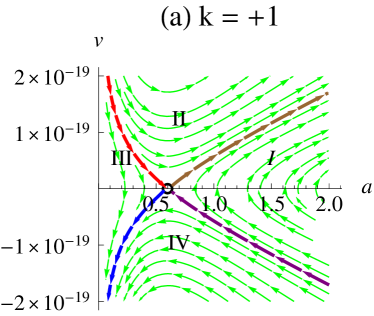
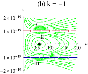
Figure 1: The phase portraits for the configuration of our universe are plotted by setting $\Omega_{\text{vac}}\simeq 0.7$, $\Omega_{m}\simeq 0.3$, $\Omega_{k}\sim 10^{-2}k$, $\Omega_{\text{rad}}\sim 10^{-4}$, and $\Omega_{\text{ds}}\sim-10^{-12}$ for (a) $k=+1$ and (b) $k=-1$. The dots on the $a$-axis represent fixed points $(a^{*},0)$ such that $1+\omega(a^{*})=0$. Actually, these figures looks the same with those of the general relativity. The crucial differences will be explicitly seen in the small scale region in Fig. 2.

In order to see how the desired evolution of the universe appears, we plot the phase portraits in Fig. 1 by setting $\Omega_{\text{vac}}\simeq 0.7$, $\Omega_{m}\simeq 0.3$, $\Omega_{k}\sim 10^{-2}k$, $\Omega_{\text{rad}}\sim 10^{-4}$, and $\Omega_{\text{ds}}\sim-10^{-12}$. Explicitly, for $k=+1$ in Fig 1(a), there is a saddle node, and the corresponding stable and unstable manifolds are shown by thick arrows. It can be also shown that the universe monotonically expanding(II) and shrinking(IV) phases, and the scale factor has a maximum(III) if the initial expansion rate is small compared to that of the phase (II). On the other hand, in the region I in Fig. 1(a), the universe can not have a scale less than that of the fixed point , i.e. $a>a^{*}\simeq 0.6$, so that the shrinking universe starts to expand before the scale factor reaches $a^{*}$. For $k=-1$ in Fig. 1(b), there is a center which is a kind of fixed points. The two straight trajectories separate closed orbits near the center from the curved trajectories, where the former case describes oscillating universes(II) while the latter one describes monotonically expanding(I) or shrinking(III) universes. Note that the oscillating universe is possible only when $\rho_{\text{tot}}<0$, and the straight line trajectories are in fact trivial solutions satisfying $\rho_{\text{tot}}=0$. As a result, the universe can experience late-time accelerated expansion after decelerated expansion in both cases (a) and (b), because current observational data indicates that the trajectory of our universe is in the region II in Fig. 1(a) or I in Fig. 1(b).

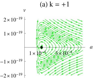
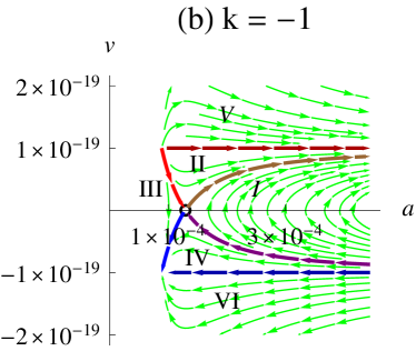
Figure 2: The phase portraits for the configuration of our universe, $\Omega_{\text{vac}}\simeq 0.7$, $\Omega_{m}\simeq 0.3$, $\Omega_{k}\sim 10^{-2}k$, $\Omega_{\text{rad}}\sim 10^{-4}$, and $\Omega_{\text{ds}}\sim-10^{-12}$, seen near the inflation era for (a) $k=+1$ and (b) $k=-1$. The dots on the $a$-axis represent fixed points $(a^{*},0)$ such that $1+\omega(a^{*})=0$.

Actually, the phase portraits in Fig. 1 are very close to the Einstein’s theory in the large scale and the large expansion rate, so we have to draw small scale behaviors to expose some differences from the general relativity. The standard lore tells us that there are no phase transitions in a small scale in the Einstein’s relativity, unless we consider an additional source such as the inflaton. However, it is possible to see a transition with the help of the dark scalar in the HL theory, which is shown in Fig. 2. The dark scalar looks like a quantum correction, in the sense that it comes from higher curvature correction and it plays a significant role at the small scale, $a\ll 1$. So, if we assume $\Omega_{\text{ds}}<0$, then we can have another fixed point near $a^{*}\sim 10^{-4}$, which gives the possibility for the first accelerated expansion. For the case of $k=+1$ in Fig. 2, there is a center near the early accelerated era. One can now see that the expanding and shrinking universe in the region III in Fig. 1(a) is actually oscillating, which means a universe with the same energy distribution as ours should oscillate if its initial expansion rate is not so large enough. As for the case of $k=-1$ in Fig. 2, there is a saddle node with stable and unstable manifolds, and the two straight trajectories whose total energy is trivial, $\rho_{\text{tot}}=0$ which separates solutions satisfying $\rho_{\text{tot}}>0$ from $\rho_{\text{tot}}<0$ solutions.

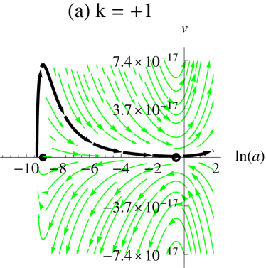
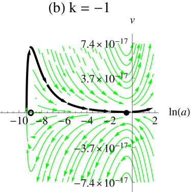
Figure 3: The phase portraits for the configuration of our universe, $\Omega_{\text{vac}}\simeq 0.7$, $\Omega_{m}\simeq 0.3$, $\Omega_{k}\sim 10^{-2}k$, $\Omega_{\text{rad}}\sim 10^{-4}$, and $\Omega_{\text{ds}}\sim-10^{-12}$, for (a) $k=+1$ and (b) $k=-1$. The thick black (curved) arrows describe the trajectory of our universe, and the dots on the $a$-axis represent fixed points $(a^{*},0)$ such that $1+\omega(a^{*})=0$.

To incorporate Fig. 1 with Fig. 2, they are plotted in terms of the logarithmic scale in Fig. 3, and then it can be shown that the universe starts from the first accelerated phase followed by a decelerated expansion phase, and ends up with the second accelerated expansion. In addition to this dynamical evolution, as seen from the two fixed points in Fig. 3, it is also possible to obtain the neutrally stable universe described by the center at the early stage of universe in Fig. 3(a) and at the late time stage of universe in Fig. 3(b). Here, ‘neutral’ means that a small perturbation does not decay into zero but remains small as time goes on.

V Discussion

We have studied the HL gravity coupled to the matter without the detailed balance condition in order to show the possibility to get the smooth phase transition from the first accelerated expansion corresponding to the early stage of the universe to the second accelerated expansion throughout the intermediate decelerated expansion assuming the energy density for the dark scalar to be negative $\rho_{\text{ds}}<0$. In spite of this negative energy contribution, the total energy density $\rho_{\text{tot}}$ is positive at any cosmological scale. Note that there have been researches which provide concrete justifications for models with negative density, in particular, a brane universe moving in a curved higher dimensional bulk space kk:mirage and a model of dark energy stemming from a fermionic condensate abc . Of course, we can confirm that there is no such a phase transition unless the dark scalar density is assumed to be negative. For instance, if we take the detailed balance condition, then it simply reduces the additional energy contribution to $\rho_{\text{vac}}=\Lambda c^{4}/8\pi G_{N}$, $\rho_{k}=-3c^{4}k/8\pi G_{N}a^{2}$, $\rho_{\text{dr}}=27c^{4}k^{2}/32\pi G_{N}\Lambda a^{4}$, $\rho_{\text{ds}}=0$ as seen from fundamental constants (5) and redefinition of coefficients (6). In this case, the first accelerated expansion does not appear, that is the reason why we did not take the detailed balance condition. In addition, it has been shown that our universe may be oscillatory even with the same density parameters of the current observation, depending on the expansion rate. Actually, the expansion rate is related to the total energy density by Eq. (17), so that small expansion rate $v$ corresponds to small $h\sim\rho_{\text{tot}}$ for a given scale factor.

On the other hand, it has been well known that if there were $\sim 60$ e-foldings of inflationary expansion, then the universe was driven to be nearly flat, removing any need for fine-tuned initial conditions. In addition, the inflationary expansion would have driven the density of magnetic monopoles to be negligible today, explaining their apparent absence. Also, our entire observable portion of the universe would have inflated from an initially small causally connected region, thereby ensuring a high degree of isotropy today. Although our analysis shows that the first accelerated expansion can be obtained by assuming $\rho_{\text{ds}}<0$, unfortunately, it should be pointed out that it does not last for 60 e-foldings. We hope this problem will be discussed elsewhere.

It is interesting to note that there exists a minimum scale $a_{\text{min}}$ obtained from $\rho_{c}\geq 0$ and $\rho_{\text{tot}}\geq 0$ with the relation $\rho_{c}=\rho_{\text{tot}}+\rho_{k}$. Note that $\rho_{\text{tot}}(a_{\text{min}})=-\rho_{k}(a_{\text{min}})>0$ and $H^{2}(a_{\text{min}})\sim\rho_{c}(a_{\text{min}})=0$ for $k=+1$, so the universe starts with a certain amount of energy and zero expansion rate, while $\rho_{\text{tot}}(a_{\text{min}})=0$ and $H^{2}(a_{\text{min}})\sim\rho_{c}(a_{\text{min}})=\rho_{k}(a_{\text{min}})>0$ for $k=-1$, so the universe starts with zero energy density and a certain expansion rate. For any case, as far as we consider the positive total energy density and the critical energy density, there should be no initial singularity problem because of the existence of the minimum scale.

The final comment is in order. The energy density and the pressure of the dark scalar which play a crucial role in this work depend on the three terms in the potential (4), $\sigma_{1}R^{3}$, $\sigma_{2}RR_{ij}R^{ij}$, $\sigma_{3}R_{i}^{j}R_{j}^{k}R_{k}^{i}$. One may think that three terms give rise to kinetic contributions so that they provide the leading spatial dependence in the gravition propagator in the UV region. What it means is that graviton modes may be unstable. However, this is not the case since they do not modify the gravition propagator. In general, the lowest metric order in curvature tensors and curvature scalars is linear, which means that the three terms are not quadratic in metric. Of course, such terms which are quadratic in curvature, $\sigma_{4}\nabla_{i}R\nabla^{i}R$, $\sigma_{5}\nabla_{i}R_{jk}\nabla^{i}R^{jk}$ in Eq. (4), will not only add interaction but also modify the propagator; however, these are irrelvant to our energy density formulae (12).

- (1) P. Hořava, JHEP 0903, 020 (2009) [arXiv:0812.4287 [hep-th]]; Phys. Rev. D 79, 084008 (2009) [arXiv:0901.3775 [hep-th]]; Phys. Rev. Lett. 102, 161301 (2009) [arXiv:0902.3657 [hep-th]].
- (2) E. M. Lifshitz, Zh. Eksp. Teor. Fiz. 11, 255 (1941); Zh. Eksp. Teor. Fiz. 11, 269 (1941).
- (3) T. Takahashi and J. Soda, Phys. Rev. Lett. 102, 231301 (2009) [arXiv:0904.0554 [hep-th]].
- (4) E. Kiritsis and G. Kofinas, Nucl. Phys. B 821, 467 (2009) [arXiv:0904.1334 [hep-th]].
- (5) S. Mukohyama, JCAP 0906, 001 (2009) [arXiv:0904.2190 [hep-th]]; S. Mukohyama, K. Nakayama, F. Takahashi and S. Yokoyama, Phys. Lett. B 679, 6 (2009) [arXiv:0905.0055 [hep-th]].
- (6) R. Brandenberger, Phys. Rev. D 80, 043516 (2009) [arXiv:0904.2835 [hep-th]].
- (7) A. Kehagias and K. Sfetsos, Phys. Lett. B 678, 123 (2009) [arXiv:0905.0477 [hep-th]].
- (8) A. Wang and Y. Wu, JCAP 0907, 012 (2009) [arXiv:0905.4117 [hep-th]].
- (9) M.-I. Park, JHEP 0909, 123 (2009) [arXiv:0905.4480 [hep-th]].
- (10) G. Leon and E. N. Saridakis, JCAP 0911, 006 (2009) [arXiv:0909.3571 [hep-th]]; S. Carloni, E. Elizalde and P. J. Silva, Class. Quant. Grav. 27, 045004 (2010) [arXiv:0909.2219 [hep-th]].
- (11) M. R. Setare and M. Jamil, JCAP 1002, 010 (2010) [arXiv:1001.1251 [hep-th]]; M. Jamil, E. N. Saridakis and M. R. Setare, The generalized second law of thermodynamics in Horava-Lifshitz cosmology, arXiv:1003.0876 [hep-th].
- (12) H. Lu, J. Mei and C. N. Pope, Phys. Rev. Lett. 103, 091301 (2009) [arXiv:0904.1595 [hep-th]].
- (13) R. G. Cai, L. M. Cao and N. Ohta, Phys. Rev. D 80, 024003 (2009) [arXiv:0904.3670 [hep-th]]; Phys. Lett. B 679, 504 (2009) [arXiv:0905.0751 [hep-th]].
- (14) E. O. Colgain and H. Yavartanoo, JHEP 0908, 021 (2009) [arXiv:0904.4357 [hep-th]].
- (15) Y. S. Myung, Phys. Lett. B 678, 127 (2009) [arXiv:0905.0957 [hep-th]]; Phys. Lett. B 684, 158 (2010) [arXiv:0908.4132 [hep-th]]; ADM mass and quasilocal energy of black hole in the deformed Hořava-Lifshitz gravity, arXiv:0912.3305 [hep-th].
- (16) R. B. Mann, JHEP 0906, 075 (2009) [arXiv:0905.1136 [hep-th]].
- (17) A. Ghodsi and E. Hatefi, Phys. Rev. D 81, 044016 (2010) [arXiv:0906.1237 [hep-th]].
- (18) E. Kiritsis and G. Kofinas, JHEP 1001, 122 (2010) [arXiv:0910.5487 [hep-th]].
- (19) B. R. Majhi, Phys. Lett. B 686, 49 (2010) [arXiv:0911.3239 [hep-th]].
- (20) R. L. Arnowitt, S. Deser and C. W. Misner, Phys. Rev. 117, 1595 (1960); “The dynamics of general relativity” in Gravitation: an introduction to current research, ed. L. Witten pp 227-265 (New York: Wiley 1962) [gr-qc/0405109].
- (21) G. Calcagni, JHEP 0909, 112 (2009) [arXiv:0904.0829 [hep-th]]; Detailed balance in Horava-Lifshitz gravity, arXiv:0905.3740 [hep-th].
- (22) M. Li and Y. Pang, JHEP 0908, 015 (2009) [arXiv:0905.2751 [hep-th]].
- (23) M. Henneaux, A. Kleinschmidt and G. L. Gomez, Phys. Rev. D 81, 064002 (2010) [arXiv:0912.0399 [hep-th]].
- (24) S. Deser, R. Jackiw and S. Templeton, Annals Phys. 140, 372 (1982) [Erratum-ibid. 185, 406 (1988); ibid. 281, 409-449 (2000)]; Phys. Rev. Lett. 48, 975 (1982).
- (25) S. H. Strogatz, “Nonlinear Dynamics and Chaos. With Applications to Physics, Biology, Chemistry, and Engineering,” Westview Press (2000) 498 p.
- (26) For the recent observational data, we refer to the five years of WMAP, whose web address is http://lambda.gsfc.nasa.gov/product/map/dr3/parameters_summary.cfm, which is actually extracted from G. Hinshaw et al. [WMAP Collaboration], Astrophys. J. Suppl. 180, 225 (2009) [arXiv:0803.0732 [astro-ph]].
- (27) A. Kehagias and E. Kiritsis, JHEP 9911, 022 (1999) [arXiv:hep-th/9910174].
- (28) S. Alexander, T. Biswas and G. Calcagni, Phys. Rev. D 81, 043511 (2010) [arXiv:0906.5161 [astro-ph.CO]].