Measures of mixing quality in open flows with chaotic advection

Abstract

We address the evaluation of mixing efficiency in experiments of chaotic mixing inside an open-flow channel. Since the open flow continuously brings new fluid into the limited mixing region, it is difficult to define relevant mixing indices, as fluid particles experience typically very different stretching and mixing histories. The repeated stretching and folding of a spot of dye leads to a persistent pattern. We propose that the normalized standard deviation of this characteristic pattern is a good measure of the mixing quality of the flow. We discuss the link between this measure and mixing of continuously-injected dye, and investigate it using an idealized map.

I Introduction

Mixing viscous fluids (whether Newtonian or not) in throughflow reactors is one of the most common and important industrial process handbook . Relevant quantitative measures of mixing efficiency are crucial for the design and evaluation of mixing systems. However, because of the wide spectrum of applications, there is not to date a universally accepted way of defining mixing efficiency Ottino1989 .

Since the 1980s, mixing at low Reynolds number has been analyzed by fluid dynamicists in the framework of chaotic advection Aref1984 ; Ottino1989 , that is, the capacity of a mixing device to generate Lagrangian trajectories that separate exponentially fast. In closed-flow mixing, that is when inhomogeneous fluid contained in a closed domain is stirred, some mixing indices stem directly from an understanding of the mechanisms of chaotic advection Ottino1989 . Among classical measures, Poincaré sections represent the region explored by a trajectory stroboscoped at discrete timesteps, and hence give the extent of the chaotic region Leong1989 ; Ottino1990 ; Jana1994 for time-periodic systems. Lyapunov exponents account for the stretching experienced by fluid particles Muzzio1991 ; Muzzio1992 ; Antonsen1996 . Topological entropy Boyland2000 ; Stremler2007 ; Gouillart2006 ; Finn2006 and braiding factors Thiffeault2005 ; Thiffeault2010 describe the entanglement of Lagrangian trajectories. Such quantities, however, are hard to link directly to the degree of homogeneity achieved by the concentration field of a scalar to be mixed. More direct indices of homogeneity include the decaying variance of the scalar field Williams1997 ; Jullien2000 ; Burghelea2004 ; Villermaux2003 ; Duplat2008 or its entropy Wang2003 . In some periodic flow configurations, the concentration field converges rapidly to a persistent pattern that repeats over time with decaying contrast Pierrehumbert1994 ; Rothstein1999 ; Voth2003 ; Liu2004 ; Tsang2005 . Such a pattern is a specific eigenmode of the Floquet operator of the advection-diffusion equation, dubbed strange eigenmode; as such it allows an intrinsic characterization of the mixing flow.

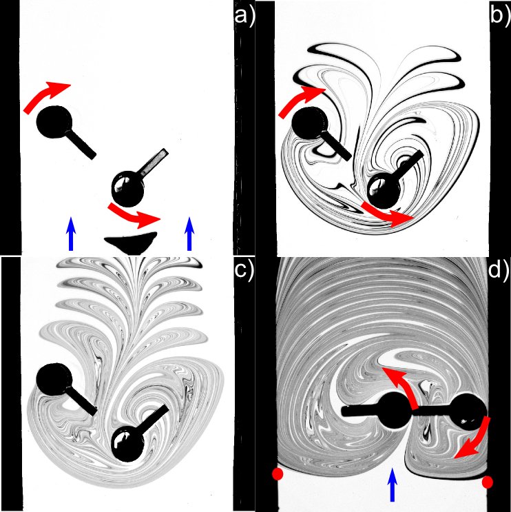
Figure 1: (a) Experimental setup: a viscous fluid in a channel is stirred by two rods moving in an eggbeater motion. A spot of black dye is injected upstream of the rods. (b) Mixing pattern observed shortly after the dye has entered the vicinity of the rods: the rods stretch some dye particles into thin filaments, while others escape downstream without being stretched and mixed. (c) Mixing pattern observed at longer times: the intensity of dye in the pattern decays with time due to diffusion – this is the ‘strange eigenmode’ regime. (d) If the rods are rotated in the opposite direction to (a–c), they prevent fluid from flowing along the channel walls. Two stagnation points (plotted as disks) on the channel sides trap fluid in their vicinity for long times. In that case, the mixing pattern occupies the whole width of the channel.

Less studied is the case of chaotic advection in open flows, in which fluid enters and then exits a limited mixing region. In this region, mechanical stirrers lead to exponential separation of fluid particles for the duration of their stay in the region (see Fig. 1(a–b)). Extensive studies of idealized open flows in 2D have focused on the properties of the underlying dynamical systems, such as the multifractal set of never-escaping trajectories – called the chaotic saddle – and its influence on Lagrangian trajectories flowing through the mixing region Jung1993 ; Pentek1995 ; Sommerer1996 ; Neufeld1998 ; Pentek1999 ; Tel2000 ; Tel2005 . Such studies focused mostly on reaction rates, and less on the mixing quality.

On the other hand, a variety of practical indices of mixing quality for open reactors can be found in the chemical engineering literature Danckwerts1952 ; Bryant1977 ; Ehrfeld1999 ; Aubin2003 ; Kukukova2009 . These indices are mostly used for turbulent flows. The intensity of segregation was defined by Danckwerts Danckwerts1952 as the variance of the scalar field in the outflow. This index characterizes directly the homogeneity, hence the quality, of the end product. Refined measures of mixing take into account the spatial scale of the scalar field as well as its variance Kukukova2009 . One can also compute the departure of the residence-time distribution (RTD) of fluid particles inside the mixer from a purely exponential RTD that characterizes a perfect mixer, in the language of chemical engineering.

In recent work Gouillart2009a , we have studied the mixing dynamics of quasi-2D free-surface channel flows stirred by two rods moving in an eggbeater protocol (see Fig. 1(a) for a picture of the rods and the channel). A spot of dye released upstream of the stirrers (Fig. 1(a)) is advected by the main channel flow and enters the mixing region where it is stretched and folded by the stirrers. Some dye particles leave the mixing region very quickly (Fig. 1(b)), while other parts of the spot remain in the mixing region longer (Fig. 1(c)). We demonstrated that, after a short time, the concentration field of the dye takes on a persistent pattern whose mean intensity decays with time Gouillart2009a . By analogy with persistent patterns in closed flows Pierrehumbert1994 ; Rothstein1999 ; Voth2003 , we called such patterns open-flow strange eigenmodes.

In the present work, we examine which information about mixing quality can be gleaned from such experiments in open flows. In particular, we investigate whether relevant measures of mixing quality can be derived from the concentration field of the strange eigenmode. This pattern is very robust, in the sense that it does not depend on the upstream location where dye was injected. It is therefore natural to use the pattern to characterize the mixing device.

The paper is organized as follows. We first describe the experimental apparatus and methods in Section II. In Section III, we describe the history of a spot of dye passing through the mixer, and the evolution of the resulting concentration field. This helps to extract relevant information from the concentration images and time series, as we describe in Section IV. In particular, we introduce a new mixing index called the eigenmode index, which is the normalized standard deviation of the persistent concentration pattern. In Section V, we relate this index to the intensity of segregation for a continuous injection of heterogeneity as introduced by Danckwerts Danckwerts1952 . The paper ends with a summary and discussion of the results.

II Mixing device configurations

Experimental data are obtained in an open-flow channel whose experimental set-up has been described in more details in Gouillart2009a ; Gouillart_thesis . Viscous fluid (cane sugar syrup) flows at a fixed rate through a long and shallow transparent channel. Two rod-stirrers (see Fig. 1) travel on intersecting circular paths at mid length of the channel, in an eggbeater protocol. Because of the low Reynolds number (see below), the mixing flow is time-periodic. We select the eggbeater protocol for the simplicity of its geometry as well as its ability to promote efficient chaotic advection. Indeed, the intersection of the trajectories of the rods ensures chaotic advection, due to stretching and folding of fluids particles. Through the stirring frequency, we control the order of magnitude of the mean number of periods spent by fluid particles inside the mixing region, which was varied between $4$ and $24$ in our experiments Gouillart2009a . Depending on the stirring frequency, Reynolds numbers range from 2 to 10, well within the laminar regime. The mixing region may be defined loosely by the region spanned by the trajectories of the stirrers; a more rigorous definition will be given in the next section.

The orientation of the trajectories of the rods (with respect to the direction of the main flow) determines the routes along which fluid flows preferentially inside the mixing region. We may rotate the rods so that they assist fluid in passing along the channel walls (Fig. 1(a)–(c)), where they drag fluid inside the mixing region only while on the upper and central part of their trajectory. Or we can rotate the rods in the opposite direction, so that fluid moving along the side walls cannot cross the mixing region, but is forced into a central funnel (Fig. 1(d)). We call the two cases respectively protocol type A and protocol type B.

We perform mixing experiments by releasing a spot of dye upstream of the rods (Fig. 1(a)). Pictures of the evolving dye pattern are taken at every period of the stirring motion with a high-resolution digital camera. Our set-up has been designed to measure quantitatively the concentration field from image processing (see Gouillart2009a ; Gouillart_thesis for more details). This requires in particular using only backlighting of the dye pattern.

III History of a dye spot

We now turn to a qualitative description of the different spacetime trajectories of fluid particles, and of the resulting dye concentration fields. The understanding we gain here will be used in the next section for defining mixing indices.

From the moment when the spot of dye is injected upstream of the rods, the fluid particles in the spot can have two types of radically different future histories: they either enter the stirring region and are mixed to some degree, or they pass through the region without being mixed. The latter behavior occurs predominantly in type A protocols, where fluid particles can flow freely along the channel walls.

The patch of fluid particles that enter the mixing region at a given period consists of dyed particles as well as some undyed white particles. After a few stirring periods, only white undyed fluid enters the mixing region. Before diffusion becomes important, the patch containing dyed particles is stretched and folded by the rods. At each stirring period, the patch moves to a new part of the mixing region, and its previous location is replaced by fresh, undyed fluid that entered the region later.

As time goes on, the original dyed patch inside the mixing region develops thin filaments as it is stretched and folded by the rods (see the filaments inside the mixing region in Fig. 1(b)). Nevertheless, as long as the width of the filaments is large enough, fluid particles of the dyed patch are not mixed by diffusion with undyed fluid particles. For example, in Fig. 1(b) most dye filaments bear the same concentration level as the initial dye spot. At every stirring period, some particles of the dyed patch leave the mixing region to compensate for fluid entering the mixing region; for short residence time they have not been mixed at all with undyed particles (see the dark filaments in the upper part of Fig. 1(b), downstream of the rods).

For longer residence times, mixing by diffusion of fluid particles with different entry times occurs at locations where the patch has been compressed down to the diffusion scale at which stretching and diffusion balance – the Batchelor scale Batchelor1959 ; Villermaux2003 ; Gouillart2008a . The Batchelor scale is given by

$$w_{\mathrm{B}}=\sqrt{\kappa/\Lambda},$$ (1)

where $\kappa$ is the diffusion coefficient and $\Lambda$ is the mean stretching (Lyapunov exponent). The scale $w_{\mathrm{B}}$ is the smallest that can be observed in the mixing pattern, and increases with $\kappa$. Once the patch has reached the scale $w_{\mathrm{B}}$, diffusion efficiently blurs its particles with particles that have different entry times. In particular, dye filaments are blurred with surrounding white fluid, and intermediate gray concentration levels appear as in Fig. 1(c). Mixing is efficient for particles of the patch that have stayed inside the mixing region at least until their filaments reach $w_{\mathrm{B}}$.

Such filaments approach the (non-elliptic) periodic points of the flow, which return to the same position after a given number of stirring periods and hence remain forever inside the mixing region. The set of all periodic points is known as the chaotic saddle for open flows Tel2000 ; Tel2005 ; Pentek1995 . It is a set of zero measure. The periodic points are typically located in between the regions occupied by the patch for short residence times, which cannot contain periodic points as they are filled with new fluid at each period. The mixing region can now be defined more precisely as the basin where the orbits of the chaotic saddle remain trapped forever, i.e., the convex hull of the set containing all these periodic orbits. Using arguments from lobe dynamics Beigie1991 , it can be shown that this set is delineated on the upstream side by the upstream boundary of the strange eigenmode pattern. On the downstream side, the extent of the mixing region is bounded by the symmetric line of the upstream boundary with respect to the horizontal axis linking the rotation center of the rods.

Dye filaments approach a periodic orbit of the chaotic saddle along the orbit’s stable manifold – the set of fluid particles that converge to the periodic orbit. Conversely, they escape an orbit along its unstable manifold – the set of particles that diverge from the orbit. The typical situation is that fluid particles in the patch approach an orbit of the chaotic saddle along its stable manifold, then recede along its unstable manifold towards another orbit, and so on until they finally escape downstream.

The dye pattern of Fig. 1(c) traces the unstable manifold of the chaotic saddle. As the unstable manifold is invariant under a full stirring period, dye always returns to the same pattern. We observe indeed in our experiments that patterns such as the one in Fig. 1(c) are persistent in time. Because of diffusion and the loss of dye downstream, the intensity of the pattern becomes weaker and weaker.

In previous work Gouillart2009a , we have shown that for protocol type A the dye pattern converges to a persistent concentration field that repeats itself periodically and whose mean is decaying exponentially with time. The concentration field obeys the equation

$$C(\mathbf{x},t=nT)=\exp(-nT/\tau)\,\tilde{C}(\mathbf{x})$$

where $\tau$ is the decay time ($1/\tau$ is the decay rate). (In general $1/\tau$ is complex, which leads to oscillations around a decaying trend; here we take its real part.) By analogy with closed flows Pierrehumbert1994 , we call $\tilde{C}(\mathbf{x})$ the strange eigenmode of the flow, as it is an eigenmode of the advection-diffusion operator Gouillart2009a . Fig. 1(c) displays an example of strange eigenmode. A physical picture of the support of the strange eigenmode (the space where $|\tilde{C}(\mathbf{x})|>0$) is given by the unstable manifold of the chaotic saddle – a fractal set of zero measure Tel2000 – fattened by diffusion into filaments of width $w_{\mathrm{B}}$. Conversely, the complement of the support of the eigenmode does not contain any periodic orbits and corresponds to the locations occupied by a patch of fluid shortly after its entry time, before it has reached the Batchelor scale. It can be seen in Fig. 2 that the short-time iterates of the dye spot are located inside the holes of the eigenmode. For example, the filamentary pattern in the mixing region in Fig. 2(a) is located in the holes of the long-time pattern of Fig. 2(c). This is also true for the fluid escaping the mixing region: the escaping filaments in the lobes of Figs. 2(a–b) are found within the holes of the pattern that periodically leaves the mixing region at long times (Fig. 2(c)). The properties of the strange eigenmode were investigated more thoroughly in Gouillart2009a .

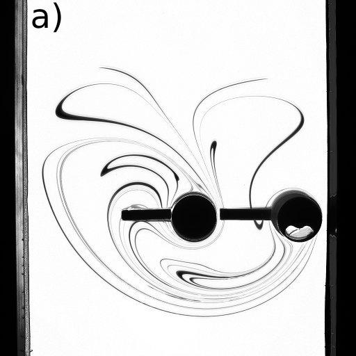
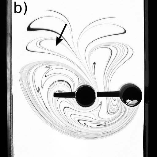
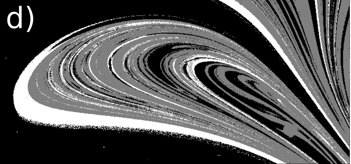
Figure 2: (a–c) Mixing pattern at periods 2, 3 and 6. Patterns (a) and (b) correspond to times shortly after the dye spot has entered the mixing region, while in (c) the dye pattern traces out the strange eigenmode. Since the flow is deterministic, the supports of the escaping lobes for the three different times are non-intersecting domains. (d) For the same experiment as (a–c), blowup of a downstream lobe, where we have superimposed the pattern of (a) and (b) (white), and the long-time pattern of (c) (gray). Filaments with short residence times are found in white ‘holes’ of the long-time pattern.

For protocol type B, however, we found that the pattern continues to evolve slightly with time and its decay does not exhibit true exponential dynamics. The reason is that, in contrast to protocol type A, the mixing pattern extends to the side walls of the channel (as in Fig. 1(d)) where the flow is less intense and stretching is slower. Therefore, dye may remain for long times in the vicinity of the walls, whereas it escapes much faster when far from the walls. As a result, the dye is increasingly located in the vicinity of the walls, and no persistent pattern is observed. Protocol type B is characterized by two specific stagnation points, whose unstable manifolds divide the upstream flow and the mixing region (red points in Fig. 1(d)). These points belong to the set of periodic orbits, but fluid approaches them much more slowly (algebraically rather than exponentially) than other periodic points. Fluid particles are therefore exchanged more rapidly between the periodic orbits of the bulk than between the wall region and the bulk. (see Gouillart2009a for more details). This prevents the onset of a persistent strange eigenmode.

In this article, we will mostly focus on the study of type A protocols, where the dye pattern converges to strange eigenmode, but we also address the case of type B protocols.

IV Mixing measures derived from the evolution of a dye spot

We now consider the different information about mixing efficiency that can be gained from our experiments, particularly from the strange eigenmode pattern.

IV.1 Location of well-mixed particles

The eigenmode pattern can be used to give predictions about the efficiency of mixing for fluid particles injected at different locations. We illustrate this with the example of two dye spots represented in Fig. 3(a), for which one would like to know if they will be efficiently mixed by the rods. The degree of mixing experienced by a fluid particle depends on its distance to the stable manifold $\mathcal{W}_{\text{s}}$ of the chaotic saddle. Particles lying within a distance $w_{\mathrm{B}}$ of the stable manifold, where $w_{\mathrm{B}}$ is the Batchelor scale, are very well mixed since, at long times, they lie within a distance $w_{\mathrm{B}}$ to the unstable manifold $\mathcal{W}_{\text{u}}$. In other words, they are eventually compressed onto the eigenmode pattern. On the other hand, particles lying further from $\mathcal{W}_{\text{s}}$ escape the region having experienced little mixing.

For our stirring configurations, an approximation to the stable manifold $\mathcal{W}_{\text{s}}$ is easily obtained: it is the mirror image (with respect to the axis of the rods’ centers) of the strange eigenmode pattern, which traces out the unstable manifold. This comes directly from (i) the time-reversibility of Stokes flows, and (ii) the symmetry of the trajectories of the rods with respect to the horizontal axis linking their rotation centers. Mirror images are therefore to be taken when both rods lie on the symmetry axis. It is then possible to predict the fate of a fluid particle from the intersection of its mirror image (blue circles in Fig. 3(a)) with the strange eigenmode. The intersecting part of the spot will be well mixed, as opposed to the non-intersecting part. In Fig. 3(a), the dye spot on the left is very well mixed as its mirror image is nested within a densely-striated lobe of the eigenmode. The dye spot on the right, however, escapes downstream without being mixed, as its mirror image has no intersection with the strange eigenmode. This has been checked experimentally.

In the same way, in Fig. 3(b), the parts of the dye spot whose mirror image is located on the strange eigenmode will be very well mixed with surrounding fluid. The other parts located on the mirror image of white filaments are less mixed – although they may experience some stretching – and will typically retain their initial upstream concentration level once advected downstream of the rods. Such considerations are useful to determine the ideal location to inject a substance that is to be mixed. This ideal location, as shown above, is inside the mirror image of the strange eigenmode.

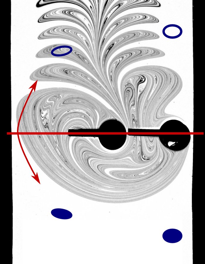
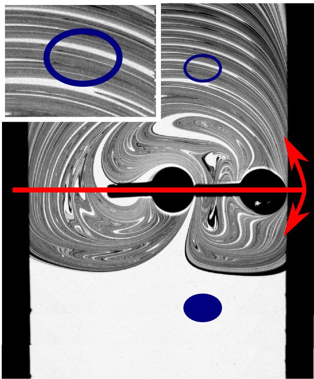
Figure 3: The fate of dye spots injected upstream (solid dark spots sketched on (a) and (b)) can be inferred from the position of their mirror image across the axis of the rods (hollow spots). (a) Example of a type A protocol. Mirror images that intersect the strange eigenmode, such as the left spot, correspond to well-mixed fluid particles. The right spot, however, has no intersection with the strange eigenmode, and will escape downstream without being caught by the rods and without being mixed. (b) Example of a type B protocol. The dye spot falls on both the support of the permanent pattern (gray patches) and its complement (white stripes), meaning that only the portion located on the support of the permanent pattern will be smeared by diffusion. It is therefore possible to obtain detailed information, such as the fraction of a dye spot that will be well-mixed, by superimposing the mirror image of the spot onto the strange eigenmode pattern.

IV.2 Distribution of residence times

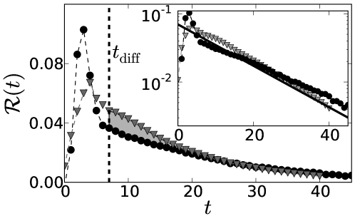
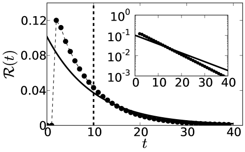
Figure 4: (a) Experiments: Residence time distribution (RTD) inside the mixing region for a typical A protocol (black circles) and B protocol (gray triangles). A vertical dashed line represents $t_{\text{diff}}$, the time where diffusion starts blurring fluid particles with different concentrations. The type A protocol is less effective at mixing than the B protocol, as reflected by the pronounced short-time peak of the RTD. Inset: RTDs on a semi-log scale display exponential tails, with slightly different slopes for each protocol type. The solid line shows the purely-exponential RTD of a perfectly random mixer. (b) Open-flow baker’s map: Circles: RTD inside the mixing region (inset: RTD on a semi-log scale). The minimum exit time is three periods. Solid line: exponential RTD of a perfectly random mixer with the same flow rate.

We now consider another quantity of interest for mixing: the residence-time distribution (RTD). Such a characterization of mixing is very common in chemical engineering and was described in detail by Danckwerts Danckwerts1952 . Since the residence time of fluid particles inside the mixing region is related to the transport properties of the flow, and, to some extent, to its mixing properties, the analysis of the RTD can be used to obtain qualitative information about mixing. We show below that an approximate quantitative measure of mixing quality can also be derived from the RTD by distinguishing between residence times that are greater or smaller than the typical time needed for diffusion to be effective.

In our experimental device, we can determine the RTD for dye particles coming from the initial dye spot by measuring the fraction of the dye that escapes the mixing region during the time interval from $t$ to $t+T$. Generally, the residence time distribution can be measured by recording the amount of dye at the outlet of the mixing region, either in model experiments or even in industrial settings. It is usually more convenient to measure the RTD than to obtain pictures of the strange eigenmode, because of obstructions or three-dimensional complexity.

In Fig. 4(a) we plot the RTD for a type A and B protocols with the same rotation speed (only the rotation direction is different). Let us give first a qualitive analyses of the two RTD’s. Two distinct regimes are observed: (i) a peak for short residence times, which is more pronounced for the type A protocol; followed by (ii) an exponential decay regime (see the inset for a semilog plot of the RTD). For the type A protocol, most dye particles that contribute to the short-time peak are in fact not entrained inside the chaotic mixing region; they flow almost unperturbed along the sides of the channel or, to a lesser extent, are entrained inside the mixing region and expelled downstream immediately. For both protocols, the onset of the exponential regime is associated with particles that are trapped in the mixing region for some time. These particles are close to the chaotic saddle, and are thus affected by their proximity to its periodic orbits Tel2000 ; Gouillart2009a (see Section III). Diffusion plays no role in this regime until particles have reached the residence time $t_{\text{diff}}$, the time at which dye filaments reach the Batchelor scale. This marks the onset of the strange eigenmode regime and of good mixing.

A first quantitative index of mixing is therefore the fraction of fluid particles that escape only after they have been stretched enough to be blurred with other particles by diffusion:

$$\alpha_{\text{diff}}=\int_{t_{\text{diff}}}^{\infty}\mathcal{R}(t)\,\text{d}t,$$ (2)

with $\mathcal{R}$ the RTD. Using this index, we see in Fig. 4(a) that the type B protocol is more efficient from a mixing perspective than the type A protocol: in the latter case, many fluid particles move along the sides the channel without being mixed.

However, this index suffers from two drawbacks. First, due to local disparities of the stretching rate, some dye filaments reach the Batchelor scale and start diffusing earlier than others. Specifically, some fluid particles may spend a long time near weakly unstable orbits and thus retain their initial concentration level, while most particles are well into the diffusive regime. It is therefore difficult to define a single diffusion time. Our choice for $t_{\text{diff}}$ in Fig. 4(a) is a pragmatic one: it is the period when most filaments start fading from pure black to intermediate gray. The second drawback is that the RTD – hence $\alpha_{\text{diff}}$ – depends on the location of the injected dye spot. More precisely, it depends on the fraction of the spot intersecting the mirror image of the strange eigenmode, as was discussed above. For type A protocols, for example, a dye spot injected at the center of the channel yields a higher mixing index than a dye spot injected close to the channel walls. This problem can be resolved by covering with dye a strip that encloses all fluid particles that enter the mixing region during one period, or by dyeing all incoming fluid from a chosen starting time, as proposed in Danckwerts1952 . These solutions present experimental difficulties. In the next subsection we introduce a more refined index based on the strange eigenmode pattern that does not suffer from the two limitations mentioned above.

In chemical engineering, distributions of residence times are often used to compute another mixing index, that is the departure from perfect mixing Danckwerts1952 . A perfect mixer is defined Danckwerts1952 ; handbook as a device where an incoming fluid particle has a constant escape probability with time. It is therefore characterized by an exponential RTD, with escape timescale $\tau_{Q}=Q/\mathcal{V}$, with $Q$ the flowrate and $\mathcal{V}$ the volume of the mixing region, according to mass conservation. Mixers that generate vigorous turbulence at high Reynolds number, for example, shuffle fluid particles randomly and may be close to perfect mixers – although the minimum exit time is always non-zero for a real system. Departures from this random mixing may be interpreted as a bypass where fluid is whisked away from the mixing zone, or dead zones where fluid is trapped for long times. One may therefore define a mixing index that measures the difference between the observed and perfectly random residence time distributions:

$$\Delta\mathcal{R}=\int_{0}^{\infty}\left|\mathcal{R}(t)-{\tau_{Q}^{-1}}\exp(-t/\tau_{Q})\right|\text{d}t.$$ (3)

For type A protocols, for example, the main contribution to $\Delta\mathcal{R}$ comes from fluid particles advected rapidly along the channel sides, and for these protocols this measure correlates well with $\alpha_{\text{diff}}$.

However, in the general case there is no direct relation between $\Delta\mathcal{R}$ and the fraction of fluid particles blurred by diffusion. Using $\Delta\mathcal{R}$ as a measure of mixing, it is even possible to find mixers that have a better mixing efficiency than the “perfect mixer.” For example, this will occur if there is a minimum residence time for fluid particles in the mixing region – this minimum time being greater than the diffusion time $t_{\text{diff}}$. This is impossible in our experiments, since the rods transport some fluid particles rapidly from the upstream side to the downstream side of the mixing region, so that very small residence times are unavoidable. A mixer with more rods arranged in an ingenious way may nevertheless increase the minimum residence time up to $t_{\text{diff}}$.

In Fig. 4(b), we show an example of such an RTD obtained with the open-flow baker’s map, where fluid particles circulate during at least three periods before they can exit the mixing region (the map was introduced in Gouillart2009a and is described in Section V.1; it is similar to an earlier map in Neufeld1998 ). As fluid particles are stretched during this residence time, this reduces the minimum scale of heterogeneities that exit the mixer, and if $t_{\text{diff}}$ is small enough, all fluid particles will be mixed by diffusion.

We conclude, therefore, that $\alpha_{\text{diff}}$ is a more relevant measure of mixing quality than $\Delta\mathcal{R}$, since the latter is not always correlated to the fraction of well-mixed particles.

IV.3 Eigenmode index

We now present a final index of mixing quality based directly on statistics of the invariant concentration field $C_{SE}$ of the strange eigenmode. We show that the normalized standard deviation of $C_{SE}$ is a relevant measure of mixing quality, and we examine how this mixing index depends on the diffusivity of dye.

IV.3.1 Definition

We define a new index of mixing called eigenmode index. The eigenmode index is defined as the standard deviation $\sigma(C_{SE})$ of the strange eigenmode divided by its mean concentration $\langle C_{SE}\rangle$:

$$\sigma_{SE}={\sigma(C_{SE})}/{\langle C_{SE}\rangle}.$$ (4)

$\sigma_{SE}$ is easily measured in decay experiments of type A protocols as the normalized standard deviation of the concentration field after a few mixing periods. This quantity becomes time-independent once the concentration field has achieved an eigenmode pattern, and is characteristic of the flow for a given value of diffusivity Gouillart2009a .

$\sigma_{SE}$ is a measure of the fluctuations of the strange eigenmode, in particular of the coverage of the fluid domain by the support of the eigenmode. The standard deviation of $C_{SE}$ will be much greater for a few isolated filaments than for a more uniform coverage of space by the eigenmode. Small values of $\sigma_{SE}$ therefore correspond to good mixing. If the strange eigenmode covers a fraction $\mathcal{A}$ of the fluid domain, $\sigma_{SE}$ can be evaluated to a first approximation as

$$\sigma_{SE}\simeq\sqrt{\frac{1-\mathcal{A}}{\mathcal{A}}}\,,$$ (5)

which is the value $\sigma_{SE}$ would take for a constant value of $C_{SE}$ over the support of the eigenmode.

IV.3.2 Dependence of the eigenmode index on the diffusivity

An important property of the eigenmode index $\sigma_{SE}$ is its specific dependence on the diffusion coefficient, or equivalently, the pixel size at which the concentration field is probed. This dependence is directly related to the multifractal properties Halsey1986 of the unstable manifold of the chaotic saddle Jung1993 ; Sommerer1996 ; Tel2000 ; Tel2005 , which is the set that supports the strange eigenmode pattern as we saw in Sec. III.

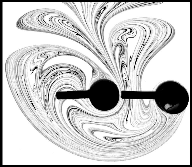
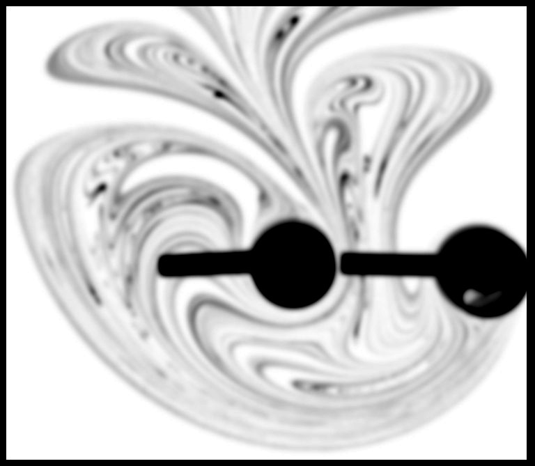
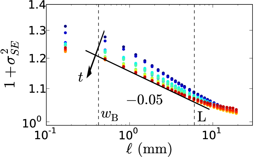
Figure 5: (a) Eigenmode pattern observed in a type A protocol. (b) Same pattern blurred at a scale $\ell=25$ pixels. (c) Evolution of $1+\sigma_{SE}^{2}(t)$ with the blurring scale $\ell$ plotted in log-log coordinates, where $\sigma_{SE}^{2}(t)$ is the rescaled variance of the dye pattern at time $t$. A power-law scaling is observed. According to Eq. (6), the small value of the slope ($0.05$) implies that the correlation dimension $D(2)$ is close to the dimension of space $d_{0}$, meaning that the pattern covers the space well. The lower cut-off at the diffusion scale $w_{\mathrm{B}}$, as well as the upper cut-off imposed by the size of the largest lobes $L$, are shown as dotted lines.

In our experiments, the temporal development of the mixing pattern resembles the construction of an (inhomogeneous) 1D Cantor set Halsey1986 . The mixing region is stretched and folded, and a fraction is removed and replaced by dye-free fluid. This is analogous to the fractal Cantor construction where one repeatedly removes a fraction of each segment – the equivalent of an iteration of the construction step being one stirring period. The fractal character of the chaotic saddle and its manifolds has been studied previously Jung1993 ; Sommerer1996 ; Tel2000 ; Tel2005 . Studies of fractal patterns due to chaotic advection have been performed in closed flows as well, for the classical closed-flow baker’s map Ott1989 ; Antonsen1991 , the blinking vortex flow Fung1991 ; Muzzio1992 , or the flow between eccentric cylinders Muzzio1992 . Here, we are interested in the implications of this fractal character for the eigenmode index.

Let us consider the evolution of $\sigma_{SE}$ when the pattern is blurred at different scales. We perform the blurring by convolving the pattern by a constant step function of width $\ell$ (in 1D for the map and in 2D for experimental data). This mimics the action of a diffusion coefficients $\kappa$ that smoothens the pattern at the diffusive scale $\ell=w_{\mathrm{B}}(\kappa)=\sqrt{\kappa/\Lambda}$ where $\Lambda$ is the mean stretching (Lyapunov exponent). We have represented in Fig. 5(a) and (b) the pattern of the strange eigenmode for a protocol of type A, and the same pattern blurred by a square kernel of size 25 pixels (the size of the initial picture in Fig. 5(a) is $1700\times 1500$ pixels). The blurring removes the finer details of the pattern by merging together neighboring strips. It follows from the fractal character of the pattern that a part of the blurred pattern of size $\delta$ is statistically equivalent to a part of the initial pattern of size $\delta/\ell$. This property implies the following power-law scaling, that we derive in Appendix A:

$$1+\sigma_{SE}^{2}\sim\ell^{D(2)-d_{0}},$$ (6)

with $d_{0}$ the dimension of space and $D(2)$ the fractal correlation dimension of the support of the eigenmode. The quantity $d_{0}-D(2)$ is a fractal codimension that measures the fraction of space that the eigenmode fails to cover.

We check the validity of the power-law scaling (6) for the eigenmode pattern of Fig. 5(a). We blur the mixing pattern at different scales (see Fig. 5(b)), and compute the resulting intensity of segregation $\sigma_{SE}$. For the domain over which $\sigma_{SE}$ is computed, we select only the filamentary pattern and not the large white strips close to the channel walls which do not participate in the stretching and folding process. In addition, we have considered the concentration field inside the mixing region rather than in the downstream lobes, as the pattern is larger and has a wider range of scales so that we expect to see the fractal scaling on a larger range. The values of $1+\sigma_{SE}^{2}$ are plotted against the blurring scale $\ell$ in Fig. 5 for different mixing times. We observe a power-law scaling for all curves over a full 1.5 decades in space, which is the signature of the ongoing stretching and folding process. All curves converge rapidly onto a single curve as a result of the convergence to a persistent pattern. At early times the effective correlation dimension is smaller than the value for the persistent eigenmode, since at the beginning of an experiment we introduce a small spot of dye and the coverage of space by the dye is less important than for the final pattern.

The lower limit of the fractal scaling range corresponds to the cut-off imposed by the physical molecular diffusion (as opposed to the artificial blurring we perform) in the experiment. In our setup, the spatial resolution of the camera is smaller than the diffusive scale so that blurring the pattern below the diffusive scale does not change it. For large values of $\ell$, no fractal scaling is expected once the blurring scale is larger than the width of the largest hole in the pattern. We verify that this scale corresponds roughly to the end of the power-law scaling range. The scaling of $1+\sigma_{SE}^{2}$ allows one to extrapolate the value of the mixing index to different values of the diffusivity. This is of practical interest for applications where the substance to be mixed has a different diffusivity from dye used in a model experiment, or when dealing with effective numerical diffusivity in a numerical simulation.

V Application to continuous injection of dye

We now turn to the investigation of open-flow mixing for the case of the continuous injection of dye.

V.1 The open-flow baker’s map

Let us first introduce an idealized 1D map that will be examined in parallel with the experiments. The map was described in previous studies Neufeld1998 ; Gouillart2009a , and serves as a toy model for chaotic advection in open flows. It is an open-flow variant of the well-studied area-preserving baker’s map Farmer1983 ; Ott1989 ; Antonsen1991 ; Fereday2002 . The action of the map is depicted in Fig. 6. The map is defined

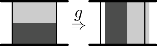
Figure 6: The action of the open-flow baker’s map: $g$ cuts the central square of a channel strip into two strips, stretches them, and re-stacks them inside the square shifted downstream to mimic advection in a channel.

on a channel-like domain, that is an infinite strip composed of a square central mixing region, and corresponding upstream and downstream regions. At each iteration, the action of the map consists of two parts: (i) a translation of the strip by a distance $U$, mimicking the global advection in an open flow; and (ii) a ‘traditional’ baker’s map inside the central mixing region. The traditional baker’s map consists of a division into two strips, which are then compressed and re-stacked, preserving area. The map therefore reproduces the main ingredients of chaotic advection in open flows: stretching, folding, and escape.

The map has the property of mapping a distribution invariant along the direction transverse to the channel into another such distribution. We restrict to such invariant distributions for the upstream concentration field, so that the action of the map amounts to a 1D transformation $g$. Specifically, we study a family of maps defined inside the unit interval by

$$g:x\mapsto g_{1}(x)\cup g_{2}(x),\qquad 0\leq x\leq 1,$$ (7a)

where

$$g_{1}(x)=U+\gamma x\,;\qquad g_{2}(x)=U+\gamma+(1-\gamma)x$$ (7b)

and the union ($\cup$) symbol in (7a) means that $g$ is one-to-two: every point $x$ has two images given by $g_{1}(x)$ and $g_{2}(x)$. The parameter $0<\gamma<1$ controls the inhomogeneity of stretching; $\gamma=1/2$ corresponding to homogeneous stretching. Diffusion is mimicked by letting the concentration evolve according to the heat equation with diffusivity $\kappa$ during a unit time interval in between iterations of the maps.

Such baker’s maps are meant to mimic type A protocols; they cannot describe type B protocols fully because of the absence of stagnation points. As was observed in the experiments, a spot of dye is rapidly transformed by the map into a persistent pattern, that is, the strange eigenmode of the map.

V.2 Case of continuous injection of dye

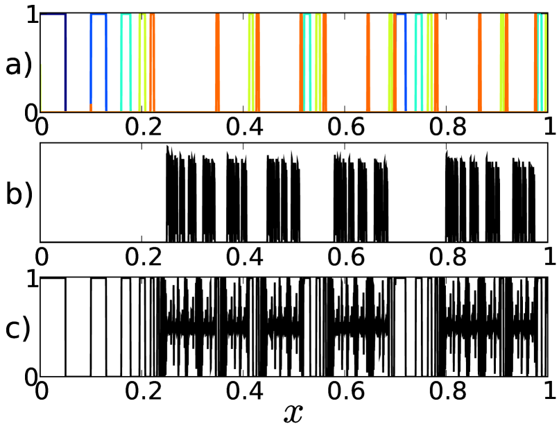
Figure 7: Mixing patterns obtained for the open-flow baker’s map: (a) For a single square-shaped blob injected at $t=0$ and short residence times (plotted with different colors, from blue to red); (b) Same initial data, but for a large number of iterations of the map, so that the concentration pattern approximates the strange eigenmode. (c) Concentration for a continuous pulse profile entering the mixing region. Large fluctuations are obtained in the same regions as in (a), that is, for short residence times, while fluctuations are much weaker on the support of the strange eigenmode visible in (b).

For a large class of industrial processes, fluid advected upstream of the mixing region is always inhomogeneous, and its concentration field measured in a sufficiently large region is characterized by stationary statistics. For example, one could realize a mixing experiment by filling one half of the upstream channel with blue dye and the other half with red dye, and try to mix together the blue and red streams inside the mixing region.

In our experiments, we focused instead on the time-localized injection of a single spot of dye. Practical reasons for this choice are twofold. First, the experimental realization of a stationary injection of dye is more problematic, especially if it has to be carried out until the downstream concentration field exhibits stationary statistics. Second, the choice of an upstream stationary field is always arbitrary: we may separate the channel into two blue and red halves, but we might also choose instead a zebra-like pattern of arbitrary wavelength. It is likely that any measure of mixing performed on such experiments will depend on some characteristics of the upstream pattern, for instance the typical lengthscale of homogeneity: a thin “premixed” zebra pattern will result in a more homogeneous downstream field than two parallel streams. In contrast, the strange eigenmode observed for a dye spot can be regarded as a unique signature of the underlying flow. We will now explain the relationship between the pattern for stationary injection of dye and the strange eigenmode resulting from a dye spot.

In the case of a stationary injection of dye, the incoming fluid can be divided in distinct patches that enter the mixing region at different times, such as the patch containing the dye spot that we considered in Sec. III. Inside the mixing region, some of these patches have been compressed onto the support of the strange eigenmode, where they are blurred with other patches by diffusion. The remainder of the mixing region is covered by patches that have not yet been mixed with others and bear concentration levels similar to the upstream levels. Therefore, high fluctuations of the concentration pattern are found on the complement of the strange eigenmode, whereas fluid is homogeneous on the strange eigenmode itself. This is illustrated with the open-flow map in Fig. 7: fluctuations of the continuous pattern are found in the holes of the strange eigenmode.

V.3 Intensity of segregation

We now describe a measure of mixing commonly used in chemical engineering for continuous mixing, the intensity of segregation, and we examine the relation between this quantity and the eigenmode index.

V.3.1 Definition

For a continuous injection of inhomogeneous fluid, the quality of mixing can be measured by the intensity of segregation

$$\sigma_{C}={\sigma_{\text{out}}}/{\sigma_{\text{in}}}\,,$$ (8)

where $\sigma_{\text{in}}$ and $\sigma_{\text{out}}$ are respectively the standard deviation of the concentration field measured on an upstream (resp. downstream) region chosen to be large enough so that $\sigma_{C}$ is time-independent. $\sigma_{C}=0$ corresponds to perfect mixing, and $\sigma_{C}\leq 1$ since mixing can only reduce fluctuations. This quantity was introduced by Danckwerts Danckwerts1952 and is widely used in chemical engineering. The quantity $1-\sigma_{C}$ can be regarded as the fraction of fluctuations suppressed in the mixing region. $\sigma_{C}$ is independent of the global intensity of scalar concentration, however it may depend on the spatial distribution of heterogeneity in the upstream pattern.

V.3.2 Link between $\sigma_{C}$ and $\sigma_{SE}$

For a poor mixer with a meager coverage of space by the eigenmode, there are typically large holes between parts of the eigenmode where the greatest fluctuations of the continuous pattern are nested. In these holes, concentration levels are of the same order as in the upstream pattern, since the pattern has been compressed only to a small extent and has not yet been smeared by diffusion. In such a case the value of $\sigma_{C}$ is expected to be close to $1-\mathcal{A}$, the fraction of space occupied by the complement of the eigenmode. Using (5), we deduce the approximate relation between $\sigma_{C}$ and $\sigma_{SE}$ in the limit of poor mixing:

$$\sigma_{SE}\simeq\sqrt{\frac{\sigma_{C}}{1-\sigma_{C}}}\;\;\text{for}\;\;\sigma_{C}\rightarrow 1.$$ (9)

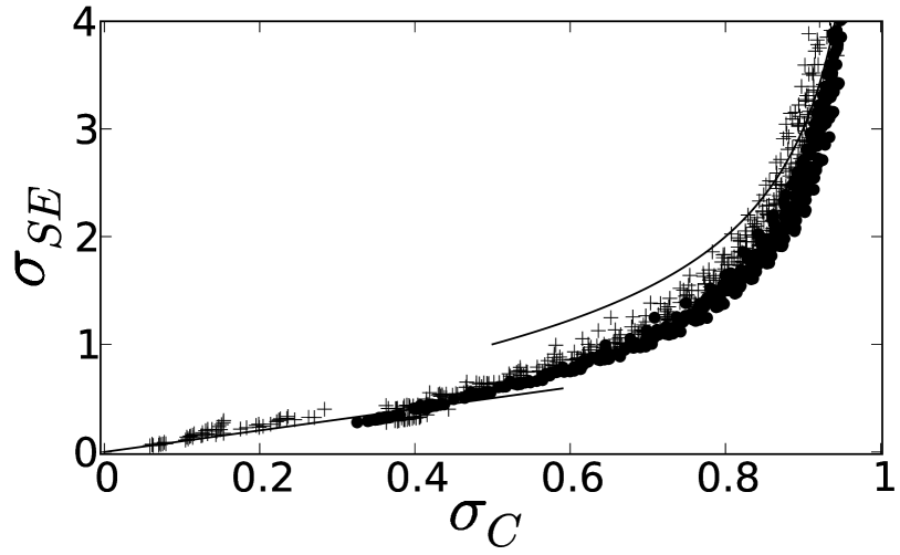
Figure 8: $\sigma_{SE}$ vs. $\sigma_{C}$ for the baker’s map (7b) for different values of the parameters $U$ (ranging from $4\times 10^{-3}$ to 0.2) and $\gamma$ (ranging from 0.3 to 0.7). $+$ and $\bullet$ symbols correspond to two different typical scales of the inlet pattern (0.4 and 1). A correlation is observed between $\sigma_{SE}$ and $\sigma_{C}$, becoming linear when they are small. The analytical relations (9) and (10) (for poor and good mixing) are plotted as solid lines.

We now use the open-flow baker’s map (7b) to investigate the strength of the correlation between $\sigma_{SE}$ and $\sigma_{C}$. The map allows us to simulate both a continuous or limited injection of scalar, and to also vary the parameters $U$ and $\gamma$ to test different mixing flows. For the continuous injection of scalar we choose a square wave of spatial period $\lambda$. $\sigma_{C}$ is measured downstream over a domain of width $100\lambda$. We compute both $\sigma_{C}$ and $\sigma_{SE}$ for 400 different maps (7b) where $U$ and $\gamma$ are uniformly distributed in the intervals $[0.02,0.2]$ and $[0.3,0.7]$, respectively. The comparison is done for two different inlet wavelengths $\lambda=0.4$ and $1$. The diffusivity is set to $\kappa=10^{-8}$, which amounts to setting the diffusive cut-off scale $\ell\sim 10^{-4}$. It is apparent in Fig. 8 that there is a strong correlation between the two mixing indices, as expected from the above qualitative arguments. The dispersion around the mean curve is quite small and decreases when the wavelength of the inlet profile is increased. We found the root-mean-square deviation around the mean curve to be $8\%$ for $\lambda=0.4$, and $5\%$ for $\lambda=1$. In comparison, we obtain a dispersion of the order of $1\%$ when plotting the intensity of segregation measured for the two values of the wavelength against each other. We find the master curve $\sigma_{SE}=f_{\lambda}(\sigma_{C})$ to depend slightly on the wavelength of the continuous profile $\lambda$, since the intensity of segregation depends on $\lambda$. Note that not all the results of our simulations of the map are plotted in Fig. 8, as for the largest values of $U$, and inhomogeneous values of stretching ($\gamma$ far from $1/2$), the strange eigenmode scarcely covers the unit interval and values of $\sigma_{SE}$ lie outside the range represented here.

The evident relationship between $\sigma_{SE}$ and $\sigma_{C}$ suggests that $\sigma_{SE}$ could be used as a convenient substitute for the intensity of segregation $\sigma_{C}$ to evaluate mixing efficiency. Additionally, the relation between the two measures can be easily understood for the two extreme regimes of very good or extremely poor mixing. Protocols with a short mean residence time (e.g., large values of $U$ for the map (7b)) are characterized by eigenmodes that cover a small fraction of space. In this limit of poor mixing, we expect $\sigma_{SE}$ and $\sigma_{C}$ to obey Eq. (9). The relation (9) is plotted in Fig. 8 for comparison with the data. It approximates the data well for $\sigma_{C}\gtrsim 0.8$, that is, for poor mixing.

More interesting for practical purposes is the case of good mixing and long mean residence times (e.g., small values of $U$ for the map), for which it is important to accurately rate protocols according to their mixing efficiency. The relationship between $\sigma_{SE}$ and $\sigma_{C}$ can be computed for the special case of an incoming square wave, which has been used in the simulations. In the limit of large residence times, many time-periods are needed before a full spatial half-wavelength of the inlet pattern has entered the mixing region. Hence, the color of injected fluid (i.e., black or white) is homogeneous for long times, as in decay experiments. The concentration pattern is close to the strange eigenmode for almost all times, except during the transition periods of the incoming fluid between dyed and undyed. Inside the mixing region, the standard deviation is therefore proportional to the mean concentration:

$$\sigma(C,t)=\alpha\,\langle C\rangle(t).$$

By definition (4), the constant of proportionality $\alpha$ equals $\sigma_{SE}$. The quantity $\langle C\rangle(t)$ oscillates around the mean value of the upstream concentration on exponential branches corresponding to the decay of the eigenmode for each color. Simple algebra then leads to the relation

$$\sigma_{SE}\simeq\frac{\sigma_{C}}{\sigma_{0}}\;\;\text{for small }\sigma_{C},$$ (10)

where $\sigma_{0}$ is the standard deviation of the upstream pattern normalized by the mean concentration ($\sigma_{0}=1$ for the square waves considered here). The above relation is verified on Fig. 8 for small values of $\sigma_{C}$.

VI Conclusions and discussion

In this article, we have examined quantitative criteria to rank open flows with chaotic advection according to their mixing efficiency. Measurements performed for a continuous injection of dye depend strongly on the spatial distribution of the incoming dye pattern, thus obscuring the inherent efficiency of the mixing device. To overcome this difficulty, we have proposed a measure of mixing based on the strange eigenmode of the flow that depends only on the mixing flow and the scalar diffusivity. Our eigenmode index is defined as the standard deviation $\sigma_{SE}$ of the eigenmode and measures approximately the area covered by fluid particles that are well mixed.

As expected, we found a good correlation between $\sigma_{SE}$ and measures of the variance for the continuous injection of a periodic pattern with a fixed lengthscale. The measure $\sigma_{SE}$ therefore ranks mixing protocols in the same order as Danckwerts’ intensity of segregation. The reason for this correlation is that fluctuations corresponding to short residence times inside the mixing region are found on the complementary subspace of the strange eigenmode. We have also noted that the dependence of $\sigma_{SE}$ on the scalar diffusivity can be predicted if the resolution of the eigenmode pattern is fine enough to obtain its fractal correlation dimension. As $\sigma_{SE}$ is easy to measure and has physical and practical relevance, we advocate the use of this new criterion for evaluating mixing efficiency.

At first sight, $\sigma_{SE}$ may seem of little use for protocols (such as our type B protocol) where a true strange eigenmode is not present because of regions of slow stretching that trap fluid particles for long times Gouillart2009a . The vicinity of “sticky” elliptical islands or no-slip solid walls are examples of regions that will be covered very slowly by an incoming spot of dye. Conversely, dye will be trapped in such regions for longer times than in the rest in the mixing region, so that no persistent eigenmode is observed Gouillart2009a . However, these regions contribute only weakly to fluctuations in the outflowing fluid for the case of a continuous injection of dye, since particles that finally escape into the rest of the chaotic region have typically experienced much more stretching than fluid particles with short residence times. Therefore, we suggest measuring $\sigma_{SE}$ at intermediate times when a quasi-persistent pattern is observed, that is, when dye filaments have reached the Batchelor scale everywhere but on these small regions of anomalous stretching. Such a measure will slightly underestimate the efficiency of mixing as compared to other protocols, because some areas not yet covered by dye will contribute to $\sigma_{SE}$, whereas they do not contribute to fluctuations of the continuous pattern. Nevertheless, this is only a small effect. $\sigma_{SE}$ should not be measured at long times when dye is mostly concentrated in the slow-stretching regions, since the fluctuations of this pattern cannot be related to those for continuous injection. Most efficient mixing protocols display either a true strange eigenmode, or a “quasi” strange eigenmode corresponding to a quasi-permanent pattern observed during a large range of intermediate times. Otherwise, a large portion of the mixing region is occupied by fluid that is trapped for long times. This may happen, for example, if the rods do not come close enough to the channel walls for a type B protocol. As the mean residence time in the mixing region is determined solely by the flowrate, this implies that there will be an increased fraction of short residence times, hence bad mixing.

Finally, we note that our study of mixing efficiency was confined to a global characterization of the homogeneity of the outgoing fluid. In particular, no characterization of the spatial fluctuations of the dye pattern has yet been proposed for open flows. It may be relevant in practical applications to measure the distribution of widths of strips of dye exiting the mixing region. Once again, this measure could be replaced by the simpler characterization of the widths of holes in the strange eigenmode, where the largest fluctuations are found. This would require the development of dedicated image processing tools.

Appendix A Scaling of $\sigma_{SE}$ with the diffusivity or box size

Let us derive here the evolution of $\sigma_{SE}$ with the box size $\ell$, using the multifractal properties of the support of the strange eigenmode.

The multifractal spectrum of a fractal set is defined as follows Halsey1986 . Let $p_{\mathcal{B}}$ be the measure in the box $\mathcal{B}$ of size $\ell$, and $q\in\mathbb{R}$. The invariance of the set at different scales implies the following scaling of the partition function $Z(q,\ell)$:

$$Z(q,\ell)=\sum_{\mathcal{B}}p_{\mathcal{B}}^{q}\sim\ell^{\tau(q)}\,.$$ (11)

The spectrum of multifractal dimensions is obtained from the spectrum $\tau(q)$ as

$$D_{q}=\tau(q)/(q-1).$$

Using the definition of $\sigma_{SE}$, we write

$$1+\sigma_{SE}^{2}=\frac{\sum_{i}C_{i}^{2}}{\bigl{(}\sum_{i}C_{i}\bigr{)}^{2}}\,,$$ (12)

with $C_{i}=C(\mathbf{x}_{i})$ the concentration level in pixel $i$. To find the multifractal scaling, instead of summing over pixels we sum the concentration over larger square boxes $\mathcal{B}$ of size $\ell$, over which the concentration has been blurred and is nearly a constant $\tilde{C}(\mathcal{B})$. Since

$$\sum_{i\in\mathcal{B}}C_{i}^{q}=\ell^{d_{0}}\tilde{C}^{q}(\mathcal{B})$$

with $d_{0}$ the dimension of space and $q\in\mathbb{R}$, we obtain

$$1+\sigma_{SE}^{2}=\frac{1}{\ell^{d_{0}}}\sum_{\mathcal{B}}\left(\frac{\tilde{C}}{\sum_{\mathcal{B}}\tilde{C}}\right)^{2}=\frac{1}{\ell^{d_{0}}}\sum_{\mathcal{B}}p^{2}_{\mathcal{B}},$$

with the measure $p_{\mathcal{B}}=\tilde{C}/\sum_{\mathcal{B}}\tilde{C}$. Using the definition of the multifractal spectrum, we finally get

$$1+\sigma_{SE}^{2}\sim\ell^{D(2)-d_{0}}.$$ (13)

References

- (1) Handbook of Industrial Mixing: Science and Practice, edited by E. L. Paul, V. Atiemo-Obeng, and S. M. Kresta (Wiley, ADDRESS, 2003).
- (2) J. M. Ottino, The Kinematics of Mixing: Stretching, Chaos, and Transport (Cambridge University Press, Cambridge, U.K., 1989).
- (3) H. Aref, “Stirring by chaotic advection,” J. Fluid Mech. 143, 1 (1984).
- (4) C. W. Leong and J. M. Ottino, “Experiments on mixing due to chaotic advection in a cavity,” J. Fluid Mech. 209, 463 (1989).
- (5) J. M. Ottino, “Mixing, chaotic advection, and turbulence,” Annu. Rev. Fluid Mech. 22, 207 (1990).
- (6) S. C. Jana, G. Metcalfe, and J. M. Ottino, “Experimental and computational studies of mixing in complex stokes flows: the vortex mixing flow and multicellular cavity flows,” J. Fluid Mech. 269, 199 (1994).
- (7) F. J. Muzzio, P. D. Swanson, and J. M. Ottino, “The statistics of stretching and stirring in chaotic flows,” Phys. Fluids A 3, 5350 (1991).
- (8) F. J. Muzzio, C. Meneveau, P. D. Swanson, and J. M. Ottino, “Scaling and multifractal properties of mixing in chaotic flows,” Phys. Fluids A 4, 1439 (1992).
- (9) T. M. Antonsen, Z. Fan, E. Ott, and E. Garcia-Lopez, “The role of chaotic orbits in the determination of power spectra of passive scalars,” Phys. Fluids 8, 3094 (1996).
- (10) P. L. Boyland, H. Aref, and M. A. Stremler, “Topological fluid mechanics of stirring,” J. Fluid Mech. 403, 277 (2000).
- (11) M. A. Stremler and J. Chen, “Generating topological chaos in lid-driven cavity flow,” Phys. Fluids 19, 103602 (2007).
- (12) E. Gouillart, J.-L. Thiffeault, and M. D. Finn, “Topological mixing with ghosts rods,” Phys. Rev. E 73, 036311 (2006).
- (13) M. D. Finn, J.-L. Thiffeault, and E. Gouillart, “Topological chaos in spatially periodic mixers,” Physica D 221, 92 (2006).
- (14) J.-L. Thiffeault, “Measuring topological chaos,” Phys. Rev. Lett. 94, 084502 (2005).
- (15) J.-L. Thiffeault, “Braids of entangled particle trajectories,” Chaos 20, 017516 (2010).
- (16) B. S. Williams, D. Marteau, and J. P. Gollub, “Mixing of a passive scalar in magnetically forced two-dimensional turbulence,” Phys. Fluids 9, 2061 (1997).
- (17) M.-C. Jullien, P. Castiglione, and P. Tabeling, “Experimental observation of batchelor dispersion of passive tracers,” Phys. Rev. Lett. 85, 3636 (2000).
- (18) T. Burghelea, E. Segre, and V. Steinberg, “Mixing by polymers: Experimental test of decay regime of mixing,” Phys. Rev. Lett. 92, 164501 (2004).
- (19) E. Villermaux and J. Duplat, “Mixing as an aggregation process,” Phys. Rev. Lett. 91, 184501 (2003).
- (20) J. Duplat and E. Villermaux, “Mixing by random stirring in confined mixtures,” J. Fluid Mech. 617, 51 (2008).
- (21) W. Wang, I. Manas-Zloczower, and M. Kaufman, “Entropic characterization of distributive mixing in polymer processing equipment,” AIChE J. 49, 1637 (2003).
- (22) R. T. Pierrehumbert, “Tracer microstructure in the large-eddy dominated regime,” Chaos Solitons Fractals 4, 1091 (1994).
- (23) D. Rothstein, E. Henry, and J. P. Gollub, “Persistent patterns in transient chaotic fluid mixing,” Nature (London) 401, 770 (1999).
- (24) W. Liu and G. Haller, “Strange eigenmodes and decay of variance in the mixing of diffusive tracers,” Physica D 188, 1 (2004).
- (25) Y.-K. Tsang, T. M. Antonsen, and E. Ott, “Exponential decay of chaotically advected passive scalars in the zero diffusivity limit,” Phys. Rev. E71, 066301 (2005).
- (26) G. A. Voth, T. C. Saint, G. Dobler, and J. P. Gollub, “Mixing rates and symmetry breaking in two-dimensional chaotic flow,” Phys. Fluids 15, 2560 (2003).
- (27) C. Jung, T. Tél, and E. Ziemniak, “Application of scattering chaos to particle transport in a hydrodynamical flow,” Chaos 3, 555 (1993).
- (28) A. Péntek, Z. Toroczkai, T. Tél, C. Grebogi, and J. A. Yorke, “Fractal boundaries in open hydrodynamical flows: Signatures of chaotic saddles,” Phys. Rev. E 51, 4076 (1995).
- (29) J. C. Sommerer, H.-C. Ku, and H. E. Gilreath, “Experimental evidence for chaotic scattering in a fluid wake,” Phys. Rev. Lett. 77, 5055 (1996).
- (30) A. Péntek, G. Károlyi, I. Scheuring, T. Tél, Z. Toroczkai, J. Kadtke, and C. Grebogi, “Fractality, chaos and reactions in imperfectly mixed open hydrodynamical flows,” Physica A 274, 120 (1999).
- (31) T. Tél, G. Károlyi, A. Péntek, I. Scheuring, Z. Toroczkai, C. Grebogi, and J. Kadtke, “Chaotic advection, diffusion, and reactions in open flows,” Chaos 10, 89 (2000).
- (32) T. Tél, A. de Moura, C. Grebogi, and G. Károlyi, “Chemical and biological activity in open flows: A dynamical system approach,” Physics Reports 413, 91 (2005).
- (33) Z. Neufeld and T. Tél, “Advection in chaotically time-dependent open flows,” Phys. Rev. E 57, 2832 (1998).
- (34) P. V. Danckwerts, “The definition and measurement of some characteristics of mixtures,” Appl. Sci. Res. A3, 279 (1952).
- (35) J. Bryant, “The characterization of mixing in fermenters,” Adv. Biochem. Eng 5, 101 (1977).
- (36) W. Ehrfeld, K. Golbig, V. Hessel, H. Lowe, and T. Richter, “Characterization of mixing in micromixers by a test reaction: single mixing units and mixer arrays,” Ind. Eng. Chem. Res 38, 1075 (1999).
- (37) J. Aubin, D. Fletcher, J. Bertrand, and C. Xuereb, “Characterization of the mixing quality in micromixers,” Chemical Engineering & Technology 26, 1262 (2003).
- (38) A. Kukukova, J. Aubin, and S. Kresta, “A new definition of mixing and segregation: Three dimensions of a key process variable,” Chemical Engineering Research and Design 87, 633 (2009).
- (39) E. Gouillart, O. Dauchot, J.-L. Thiffeault, and S. Roux, “Open-flow mixing: Experimental evidence for strange eigenmodes,” Phys. Fluids (2009).
- (40) E. Gouillart, Ph.D. thesis, Université Pierre et Marie Curie, Paris, 2007.
- (41) E. Gouillart, O. Dauchot, B. Dubrulle, S. Roux, and J.-L. Thiffeault, “Slow decay of concentration variance due to no-slip walls in chaotic mixing,” Phys. Rev. E78, 026211 (2008).
- (42) G. K. Batchelor, “Small-scale variation of convected quantities like temperature in turbulent fluid: Part 1. General discussion and the case of small conductivity,” J. Fluid Mech. 5, 113 (1959).
- (43) D. Beigie, A. Leonard and S. Wiggins, “A global study of enhanced stretching and diffusion in chaotic tangles,” Phys. Fluids 3, 1039 (1991).
- (44) T. C. Halsey, M. H. Jensen, L. P. Kadanoff, I. Procaccia, and B. I. Shraiman, “Fractal measures and their singularities: The characterization of strange sets,” Phys. Rev. A 33, 1141 (1986).
- (45) E. Ott and T. M. Antonsen, “Fractal measures of passively convected vector fields and scalar gradients in chaotic fluid flows,” Phys. Rev. A 39, 3660 (1989).
- (46) T. M. Antonsen and E. Ott, “Multifractal power spectra of passive scalars convected by chaotic fluid flows,” Phys. Rev. A 44, 851 (1991).
- (47) J. C. H. Fung and J. C. Vassilicos, “Fractal dimensions of lines in chaotic advection,” Phys. Fluids 3, 2725 (1991).
- (48) J. D. Farmer, E. Ott, and J. A. Yorke, “The dimension of chaotic attractors,” Physica D 7, 153 (1983).
- (49) D. R. Fereday, P. H. Haynes, A. Wonhas, and J. C. Vassilicos, “Scalar variance decay in chaotic advection and Batchelor-regime turbulence,” Phys. Rev. E 65, 035301 (2002).