A New Radio Loudness Diagnostic for Active Galaxies: a Radio-To-Mid-Infrared Parameter

Abstract

We have studied the relationship between the nuclear (high-resolution) radio emission, at 8.4 GHz (3.6 cm) and 1.4 GHz (20 cm), the [O IV] $\lambda$25.89 $\micron$, [Ne III] $\lambda$15.56 $\micron$ and [Ne II] $\lambda$12.81 $\micron$ emission lines and the black hole mass accretion rate for a sample of Seyfert galaxies. In order to characterize the radio contribution for the Seyfert nuclei we used the 8.4GHz/[O IV] ratio, assuming that [O IV] scales with the luminosity of the AGN. From this we find that Seyfert 1’s (i.e., Seyfert 1.0’s, 1.2’s, and 1.5’s) and Seyfert 2’s (i.e., Seyfert 1.8’s, 1.9’s, and 2.0’s) have similar radio contributions, relative to the AGN. On the other hand, sources in which the [Ne II] emission is dominated either by the AGN or star formation have statistically different radio contributions, with star formation dominated sources more “radio loud”, by a factor of $\sim 2.8$ on average, than AGN dominated sources. We show that star formation dominated sources with relatively larger radio contribution have smaller mass accretion rates. Overall, we suggest that 8.4GHz/[O IV], or alternatively, 1.4GHz/[O IV] ratios, can be used to characterize the radio contribution, relative to the AGN, without the limitation of previous methods that rely on optical observables.

1 Introduction

Active galactic nuclei (AGN) are among the most powerful objects in the universe with an extraordinary amount of energy released from their unresolved nuclei. Active super-massive black holes (SMBH) in the center of these galaxies are responsible for the tremendous diversity in their observed energy emission (e.g., Rees, 1984; Sanders et al., 1989; Peterson & Wandel, 2000; Peterson et al., 2004). Despite the fact that the unified scheme of AGN has been able to explain the observed type I/II dichotomy (see Antonucci, 1993, for a review), it is clear that by looking at different wave bands there are additional parameters that can complement our current understanding of AGN classification other than to be attributed solely to a viewing angle difference (e.g., Maiolino et al., 1997; González Delgado et al., 2001; Buchanan et al., 2006; Meléndez et al., 2008b). Therefore, in order to unveil and understand the complexity of these sources, ones needs to rely on multiwavelength studies. In particular, the radio and mid-infrared emissions are basically unaffected by dust extinction which make these energy bands ideal to investigate the nature of the “hidden” nuclear engine. On the other hand, extended radio emission and low-ionization mid-infrared emission lines are excellent tracers of star formation activity when properly calibrated (e.g., Condon, 1992; Ho & Keto, 2007).

Furthermore, the strength of the observed radio emission in AGN seems to follow a bimodal distribution falling into “radio loud” and “radio quiet” sources (e.g., Miller et al., 1990; Xu et al., 1999). Historically, the dividing criterion for the AGN radio loudness was adopted to be the ratio between the radio emission, at the most commonly used frequency of 5 GHz, and the optical continuum at $\sim 4400$ Å, i.e., the radio-to-optical parameter, ${\rm R=L_{\nu}{\rm(6{\rm cm})}/L_{\nu}({\rm B})}$ (e.g., Kellermann et al., 1989; Visnovsky et al., 1992). This convention to quantize the radio loudness of a source is straightforward when the contribution from the host galaxy does not affect the observed radio and optical components of the AGN, for example in quasars, where the active nucleus overpowers the underlying galaxy. In the case of Seyfert galaxies the quantification of their radio loudness could be more subtle. Ho & Peng (2001) found that most Seyfert 1 galaxies, previously classified as radio-quiet, fall into the radio loud regime when the nuclear component for the radio-to-optical parameter is properly measured. However, even with a resolution of few arcseconds, the nuclear component of the optical luminosity could be contaminated by star formation and is strongly affected by dust extinction that may lead to an erroneous AGN characterization.

Previous multiwavelength studies have shown statistically significant correlations between the radio core luminosity and purportedly orientation-independent measures of the intrinsic luminosity of the active nuclei, which suggests a common mechanism at nuclear (subkiloparsec) scales, , e.g., accretion onto the black hole (e.g., Rawlings et al., 1989; Xu et al., 1999; Ho, 2002; Diamond-Stanic et al., 2009). On the other hand, the correlations between extra-nuclear radio emission and the far-infrared (FIR) luminosity of the galaxy suggest a circumnuclear starburst as the common cause for these observables (e.g., Condon et al., 1982; Condon & Broderick, 1988; Baum et al., 1993; Roy et al., 1998). In this regard, early studies suggested two possible scenarios for the origin of the compact radio fluxes observed in radio quiet sources: either the radio emission is associated with a nuclear starburst or generated by relativistic electrons accelerated by a low-power jet (similar to radio loud sources), with high-resolution radio-imaging observations favoring the latter (e.g., Blundell & Beasley, 1998). More recently, the good correlation between the X-ray and the radio luminosities raise the possibility that radio emission in radio quiet sources may have a coronal origin (Laor & Behar, 2008). All these exemplify that the radio properties of the AGN are diverse and can be intimately associated with fundamental parameters of the active galaxies, such as the black hole masses, mass accretion rates, and host galaxy morphology (e.g., Xu et al., 1999; Laor, 2000; Wu & Han, 2001).

Recently, Meléndez et al. (2008a) found a tight correlation in Seyfert 1 galaxies between the [O IV] $\lambda$25.89 $\micron$ and the X-ray 14-195 keV continuum luminosities from Swift/BAT observations (Markwardt et al., 2005; Tueller et al., 2008). A weaker correlation was found in Seyfert 2 galaxies, which was attributed to the effect of Compton scattering in the 14-195 keV band. These results suggest that [O IV] is a truly isotropic property of AGNs, given its high ionization potential and that it is basically unaffected by reddening, meaning that the [O IV] strength directly measures the AGN power. This result has been later confirmed in more complete samples (Rigby et al., 2009, Weaver et al. submitted to ApJ). Moreover, the strong correlation found between [O IV] and the high-ionization ($\sim$97 eV) [Ne V] $\lambda$14.32/24.32 $\micron$ emission is a further argument for [O IV] being a good indicator for the intrinsic luminosity of the AGN (e.g., Dudik et al., 2009; Goulding & Alexander, 2009, Weaver et al. submitted to ApJ). It is the primary goal of this paper to examine the physical relationship between the nuclear radio emission and the mid-infrared emission line luminosities in Seyfert galaxies. We use high-resolution radio continuum measurements and the [O IV] emission line to investigate the radio loudness of the Seyfert nuclei and the black hole mass accretion rate for a sample of Seyfert galaxies.

2 The Sample

We have obtained, from the literature, observations with the Very Large Array (VLA) in A-configuration at 8.4-GHz (see Thompson et al., 1980, for instrumental details), with a resolution of $0.25$^′′ and the largest detectable size of $3.5$^′′, for the radio quiet sources in the sample of Seyfert galaxies presented in Meléndez et al. (2008b). This sample of Seyfert galaxies includes compilations from Deo et al. (2007), Tommasin et al. (2008), Sturm et al. (2002), Weedman et al. (2005) and from our analysis of archival spectra observed with the Infrared Spectrograph (IRS) on board Spitzer Space Telescope (Werner et al., 2004) (see Appendix). For comparison, we also have obtained from the literature high resolution 1.4 GHz data observed with the VLA in B configuration, which has a resolution of $\sim 5$^′′, thus only encompassing the nucleus. Figure 1 shows the good correlation between the 1.4 GHz and 8.4 GHz fluxes and the distribution of their spectral indices. The good correlation is expected as in high-resolution both fluxes are dominated by the active nucleus. One needs to consider that the spectral indices may provide a lower limit to the nuclear component, as the 1.4 GHz B-configuration fluxes could include some extranuclear emission, thus a possible contamination from star formation. In this regard, and in order to complete this set of high-resolution 8.4 GHz fluxes, we extrapolated high-resolution observations at different frequencies to 8.4GHz by assuming a conservative $f_{\nu}\propto\nu^{-0.7}$, as determined by the spectral indices distribution. Finally, in order to check on the effect of radio emission regions on scales bigger than that sampled by the VLA in B configuration at 1.4 GHz, we compared these data with fluxes from the NRAO VLA Sky Survey (NVSS), which has a resolution of $\sim 45$^′′. We found an excellent correlation between VLA in B configuration at 1.4 GHz and NVSS fluxes, $r_{s}=0.89,~{}P_{r}<10^{-6}$, that suggests that, in our sample, compact nuclear regions dominate over large-scale extranuclear emission regions.

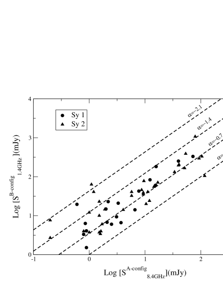
Figure 1: Correlation between the high-resolution 1.4 GHz and 8.4 GHz. The dashed lines indicate the flux density relationship expected for different spectral indices in Seyfert 1 (circles) and Seyfert 2 (triangles) galaxies.

The final sample includes 29 Seyfert 1’s (i.e., Seyfert 1.0’s, 1.2’s, and 1.5’s) and 59 Seyfert 2’s (i.e., Seyfert 1.8’s, 1.9’s, and 2.0’s), which are listed in Table 1. There are six upper limits for the 8.4 GHz emission, two Seyfert 1 galaxies and four Seyfert 2 galaxies. Note that it was not possible to find 8.4 GHz high-resolution fluxes for all the galaxies in the sample first presented by Meléndez et al. (2008b). The total radio luminosity, ${\rm L_{8.4GHz}\equiv\nu L_{\nu}{\rm(8.4GHz)}}$ (ergs/s), and the different mid-infrared emission-line luminosities are calculated from the fluxes assuming $H_{o}=71{\rm kms^{-1}Mpc^{-1}}$ and a deceleration parameter $q_{o}=0$. At the median redshift for the sample, $z=0.02$, 1^′′ represents $\sim$400 pc. Furthermore, for a full aperture extraction, Spitzer short-low (low-resolution, R$\sim 60-127$) and short-high (high-resolution, R$\sim 600$) slits will sample, in the dispersion direction, a region equivalent to the region sampled by the VLA in B-configuration at 1.4-GHz.

Table 1: The Infrared Sample of Seyfert Galaxies

Name	$z$	Type	${\rm L_{8.4GHz}}$	${\rm L_{1.4GHz}}$	$\log{\rm M_{BH}}$	$\log{\rm L_{bol}/L_{Edd}}$	${\rm R_{[OIV]}}$	${\rm R_{[NeIII]}}$	${\rm R_{[NeII]}}$	MC	Ref.
			($\log$ ergs ${\rm s^{-1}}$)		$(M/M_{\odot})$
CGCG381-051	0.0307	2	38.02				-2.30	-2.77	-3.53	S	2
Circinus	0.0014	2	37.10a		6.23b	-0.19	-3.38	-3.08	-3.51	S	8,24
ESO012-G021	0.0300	1	$<$39.08a				-2.42	-2.03	-2.30	A	9
ESO103-G035	0.0133	1	38.79a		7.15	-0.47	-2.34	-2.20	-2.09	A	10,25
ESO141-G055	0.0360	1	$<$39.24a		7.10b	-0.23	-2.08	-1.97	-1.57	A	9,26
ESO541-G012	0.0566	2	38.69				-2.87	-2.48	-2.44	A	2
ESO545-G013	0.0337	1	38.65				-2.82	-2.77	-2.76	S	2
I Zw 1	0.0611	1	38.78	38.88	7.26d	-0.15	-2.77	-3.24	-2.96	S	3,14,27
IC4329A	0.0161	1.2	38.86	38.67	7.00e	0.32	-2.91	-2.55	-2.20	A	2,13,28
IRAS00198-7926	0.0728	2	40.59a		8.44b	-0.28	-2.01	-1.64	-1.28	A	11,29
IRAS00521-7054	0.0689	2	40.64a		8.45b	-0.92	-1.33	-1.30	-1.16	S	11,30
IRAS01475-0740	0.0177	2	39.89		6.09	0.14	-0.79	-1.02	-1.15	S	1,31
IRAS04385-0828	0.0151	2	38.50		8.77b	-2.44	-2.27	-2.45	-2.58	S	1,32
IRAS15091-2107	0.0446	1	39.46	39.81	7.00d	0.69	-2.68	-2.40	-2.25	A	2,16,33
IRAS15480-0344	0.0303	2	39.28	39.06	8.22b	-0.83	-2.56	-2.20	-1.87	A	1,15,29
IRAS22017+0319	0.0611	2	39.15		8.07b	-0.13	-3.24	-2.92	-2.55	A	2,30
MCG-2-40-4	0.0252	2	38.54				-2.85	-2.85	-2.74	A	2
MCG-2-58-22	0.0469	1.5	39.74a		7.18b	0.08	-1.96	-1.95	-1.54	A	4,26
MCG-2-8-39	0.0299	2	38.52		7.85	-0.82	-2.95	-2.77	-2.62	A	1,31
MCG-3-58-7	0.0315	2	38.22				-3.20	-3.12	-2.82	A	2
MCG-5-13-17	0.0126	1.5	37.86	37.46	7.94	-1.77	-2.76	-2.79	-2.72	A	1,13,31
MCG-6-30-15	0.0077	1.2	36.99	36.86	6.81	-0.78	-3.49	-2.74	-2.94	A	13,13,31
MRK 3	0.0140	2	39.45	39.80	8.36	-0.86	-2.50	-2.49	-2.11	A	13,13,31
MRK 6	0.0188	1.5	39.41	39.44	7.64b	-0.50	-2.18	-2.15	-1.86	A	1,13,26
MRK 9	0.0399	1.5	38.38	38.21	7.46b	-0.62	-2.92	-2.45	-2.68	A	2,15,26
MRK 79	0.0222	1.2	38.26	38.35	7.72e	-0.43	-3.48	-3.08	-2.77	A	1,15,28
MRK 273	0.0378	2	39.95	39.77	8.22	-0.37	-2.36	-2.18	-2.28	S	2,15,31
MRK 334	0.0219	1.8	38.12	38.53	6.51b	0.24	-3.08	-3.31	-3.38	S	3,12,34
MRK 335	0.0258	1.2	38.41	38.14	7.15e	-0.57	-2.62	-2.13	-2.07	A	3,13,28
MRK 348	0.0150	2	40.15	39.32	6.83	-0.21	-0.92	-0.93	-0.65	A	2,13,31
MRK 471	0.0342	1.8	38.55a	38.16	7.74	-1.17	-2.47	-2.34	-2.34	A	12,12,35
MRK 509	0.0344	1.2	39.17a	38.72	8.16e	-0.86	-2.58	-2.47	-2.37	A	4,17,28
MRK 573	0.0172	2	38.01	38.11	7.28	-0.02	-3.69	-3.18	-2.91	A	3,13,36
MRK 609	0.0345	1.8	39.20a		6.80f	0.08	-2.13	-2.18	-2.30	S	4,37
MRK 622	0.0232	2	38.23	38.00	6.92	-0.30	-2.85	-2.75	-2.62	A	13,13,36
MRK 817	0.0315	1.5	38.82		7.69e	-1.02	-2.30	-2.12	-2.22	A	3,28
MRK 883	0.0375	1.9	39.43a	38.94	8.15	-1.10	-2.06	-1.96	-2.10	S	12,12,25
MRK 897	0.0263	2	38.65		7.42	-1.89	-1.32	-2.17	-2.91	S	2,25
NGC 424	0.0118	2	38.48	38.00	7.54	-1.26	-2.26	-2.32	-2.18	A	2,13,25
NGC 513	0.0195	2	37.92	38.68	7.65	-1.22	-2.95	-2.90	-3.04	S	2,13,36
NGC 931	0.0167	1.5	37.78		7.64	-0.67	-3.63	-3.34	-2.90	A	1,36
NGC 985	0.0431	1	39.11a	38.58	8.05d	-0.76	-2.63	-2.58	-2.36	A	4,15,38
NGC 1068	0.0038	2	39.30	39.24	7.56	-0.24	-2.47	-2.40	-2.04	A	3,15,25
NGC 1125	0.0109	2	38.40		7.01	-0.58	-2.47	-2.50	-2.44	A	2,25
NGC 1194	0.0136	1	37.48	36.92	7.32b	-1.02	-3.27	-3.08	-2.82	A	2,15,39
NGC 1320	0.0135	2	37.52	37.31	7.18	-0.52	-3.58	-3.03	-3.03	A	2,13,36
NGC 1365	0.0055	1.8	37.70	37.54	7.62g	-1.03	-3.34	-2.89	-3.33	S	2,18,40
NGC 1667	0.0152	2	37.80	37.41	7.62	-1.29	-2.98	-3.18	-3.31	S	2,19,25
NGC 2639	0.0111	1.9	39.42	38.59	7.94	-2.48	-0.48	-0.78	-1.05	S	2,19,41
NGC 2992	0.0077	2	38.64	38.57	7.87	-1.19	-2.48	-2.26	-2.21	A	2,20,25
NGC 3079	0.0037	2	38.37	38.09	7.97	-2.39	-1.66	-1.55	-2.28	S	3,15,41
NGC 3227	0.0039	1.5	37.51	37.57	7.63e	-1.78	-2.77	-2.85	-2.80	A	3,15,28
NGC 3516	0.0088	1.5	37.64	37.35	7.63e	-1.27	-3.16	-3.00	-2.49	A	3,13,28
NGC 3660	0.0123	2	$<$36.92		6.83	-1.21	-3.16	-2.77	-3.41	S	2,25
NGC 3783	0.0097	1.5	38.14		7.47e	-1.14	-2.65	-2.59	-2.49	A	1,28
NGC 3786	0.0089	1.8	37.16	37.46	7.53	-1.46	-3.35	-3.15	-3.12	A	3,20,36
NGC 3982	0.0037	2	36.29	36.22	6.37	-2.05	-2.47	-2.87	-3.38	S	3,15,41

Table 2: continued

The Infrared Sample of Seyfert Galaxies Name $z$ Type ${\rm L_{8.4GHz}}$ ${\rm L_{1.4GHz}}$ $\log{\rm M_{BH}}$ $\log{\rm L_{bol}/L_{Edd}}$ ${\rm R_{[OIV]}}$ ${\rm R_{[NeIII]}}$ ${\rm R_{[NeII]}}$ MC Ref. ($\log$ ergs ${\rm s^{-1}}$) $(M/M_{\odot})$ NGC 4051 0.0023 1.5 35.77 36.50 6.28^e -1.16 -3.80 -3.66 -3.53 A 3,15,28 NGC 4151 0.0033 1.5 38.16 38.04 7.12^e -0.81 -2.61 -2.61 -2.35 A 3,15,28 NGC 4388 0.0084 2 38.08 37.88 7.10 0.04 -3.50 -3.09 -3.03 A 3,15,25 NGC 4501 0.0076 2 $<$36.32 36.67 7.81 -2.54 -3.40 -3.45 -3.62 S 2,15,41 NGC 4507 0.0118 1.9 38.11 7.56 -0.94 -2.95 -2.83 -2.90 A 5,25 NGC 4748 0.0146 1 37.70 6.44 0.69 -3.88 -3.16 -2.83 A 5,31 NGC 4941 0.0037 2 37.00 36.77 6.88 -1.46 -2.86 -2.84 -2.63 A 1,19,25 NGC 4968 0.0099 2 38.01 37.98 7.25 -0.90 -2.79 -2.69 -2.69 A 2,13,25 NGC 5005 0.0032 2 37.20 37.14 7.87 -2.73 -2.39 -2.34 -2.91 S 2,15,41 NGC 5256 0.0279 2 39.32 39.12 6.92^b 0.65 -2.70 -2.48 -2.80 S 2,15,26 NGC 5347 0.0078 2 37.24 36.79 6.79 -1.30 -2.69 -2.49 -2.59 A 1,19,36 NGC 5506 0.0062 1.9 38.86 38.58 6.88 -0.12 -2.35 -1.93 -1.77 A 1,15,25 NGC 5548 0.0172 1.5 38.07 38.31 7.83^e -1.29 -2.91 -2.88 -2.34 A 3,13,28 NGC 5643 0.0040 2 37.22 37.29 6.79 -0.64 -3.38 -3.06 -2.97 A 6,21,25 NGC 5929 0.0083 2 38.32 38.17 7.22 -1.65 -1.70 -1.80 -2.17 S 3,15,31 NGC 5953 0.0066 2 36.93 37.92 6.79 -0.93 -3.38 -3.36 -4.06 S 2,15,25 NGC 6240 0.0245 2 39.77 39.85 9.15 -1.80 -2.03 -2.14 -2.64 S 7,7,42 NGC 6300 0.0037 2 36.82 6.92 -1.31 -3.24 -2.84 -2.83 A 6,25 NGC 6890 0.0081 2 37.25 37.29 7.07 -1.37 -2.90 -2.72 -2.95 A 2,19,25 NGC 7130 0.0162 2 38.93 7.52 -0.58 -2.45 -2.39 -2.67 S 2,31 NGC 7213 0.0058 1.5 39.06 7.99 -2.86 -0.51 -0.93 -1.22 S 1,36 NGC 7314 0.0048 1.9 36.84 6.03 0.02 -3.65 -3.17 -2.84 A 2,25 NGC 7469 0.0163 1.5 38.89 39.17 7.09^e 0.04 -2.69 -2.43 -3.21 S 3,22,28 NGC 7582 0.0053 2 38.41 38.14 7.40 -0.84 -2.60 -2.19 -2.53 A 2,21,25 NGC 7590 0.0053 2 $<$36 6.90 -1.83 -3.52 -3.32 -3.67 A 2,25 NGC 7603 0.0295 1.5 38.73 38.75 8.08 -1.40 -2.40 -2.40 -2.60 S 2,15,36 NGC 7674 0.0289 2 39.79 39.70 7.56 -0.08 -2.14 -2.14 -1.73 A 3,23,36 TOL1238-364 0.0109 2 38.32 $\geq$38.45 6.83 -0.79 -2.17 -2.62 -2.68 S 2,19,31 UGC 7064 0.0250 1.9 $<$37.36 38.16 -4.01 -3.77 -3.62 A 2,15 UGC 12138 0.0250 1.8 38.34 7.16 -0.43 -2.84 -2.70 -2.27 A 5,31 UM 146 0.0174 1.9 38.54 6.19 -0.52 -1.58 -1.89 -1.76 S 3,31 ^a 8.4 GHz High-resolution data was unavailable, thus we extrapolated measurements from other wavelengths assuming, $f_{\nu}\propto\nu^{-0.7}$

^b Values for the stellar velocity dispersion from the FWHM of [O III] $\lambda~{}5007$, $\sigma_{[OIII]}$

^c Maser Kinematics

^d Virial Theorem

^e Reverbertation Mapping

^f From broad ${\rm H_{\alpha}}$ emission

^g $M_{BH}-\sigma_{bulge}$ relationship

Note: The luminosities were calculated from the fluxes using $H_{o}=71{\rm kms^{-1}Mpc^{-1}}$ and a deceleration parameter $q_{o}=0$ with redshift values taken from NED. ${\rm R_{[OIV]}}$, ${\rm R_{[NeIII]}}$ and ${\rm R_{[NeII]}}$ are the 8.4GHz-to-mid-infrared parameters. The last two columns show the main contribution (MC) to the [Ne II] emission line (A=AGN and S=Star Formation) and the references for the observed high-resolution 8.4 GHz and 1.4 GHz emission fluxes and black holes masses ${\rm M_{BH}}$, respectively. Most of the values for the BH masses were calculated by using the relationship between the black hole mass and the stellar velocity dispersion (Tremaine et al., 2002), unless noted.

References: (1) Schmitt et al. (2001), (2) Thean et al. (2000), (3) Kukula et al. (1995), (4) Ulvestad & Wilson (1984a), (5) Schmitt et al. 2009, in prep, (6) Morganti et al. (1999), (7) Colbert et al. (1994), (8) Davies et al. (1998), (9) Roy et al. (1994), (10) Heisler et al. (1998), (11) Roy et al. (1998), (12) Ulvestad (1986), (13) Nagar et al. (1999), (14) Condon et al. (1987), (15) Becker et al. (1995), Faint Images of the Radio Sky at Twenty Centimeters (FIRST) survey, (16) Ulvestad et al. (1995), (17) Unger et al. (1987), (18) Sandqvist et al. (1995), (19) Ulvestad & Wilson (1989), (20) Ulvestad & Wilson (1984b), (21) Morris et al. (1985), (22) Laine et al. (2006), (23) Menon & Hickson (1985), (24) Greenhill et al. (2003), (25) Cid Fernandes et al. (2004), (26) Whittle (1992), (27) Kawakatu et al. (2007), (28) Peterson et al. (2004), (29) Lipari et al. (1991), (30) Young et al. (1996), (31) Garcia-Rissmann et al. (2005), (32) Wang et al. (2007), (33) Ohta et al. (2007), (34) Dahari & De Robertis (1988), (35) Ho (2007), (36) Nelson & Whittle (1995), (37) Greene & Ho (2007), (38) O’Neill et al. (2005), (39) Kirhakos & Steiner (1990), (40) Risaliti et al. (2009), (41) Ho et al. (2009), (42) Doyon et al. (1994)

In order to confirm that our sample is not biased in terms of luminosities we compared the different luminosities for both the mid-infrared emission lines and the radio continuum luminosities for the two groups of galaxies. The histograms of [Ne II], [Ne III] and [O IV] luminosities and 8.4 GHz continuum luminosities are presented in Figure 2 with the results from the Kolmogorov-Smirnov (K-S) test presented in Table 3. This table also includes information about the numbers of Seyfert 1 and Seyfert 2 galaxies, median values and standard deviations of the mean for the measured quantities. For the 8.4 GHz continuum the K-S test returns a $\sim 82.0\%$ probability of the null hypothesis (i.e., that there is no difference between Seyfert 1 and Seyfert 2 galaxies), or in other words, two samples drawn from the same parent population would differ this much $\sim 82.0\%$ of the time. For the [Ne II], [Ne III] and [O IV] luminosity distributions the K-S test returns a $\sim 96.9\%$, $\sim 47.9\%$ and $\sim 27.8\%$ probability of the null hypothesis, respectively.

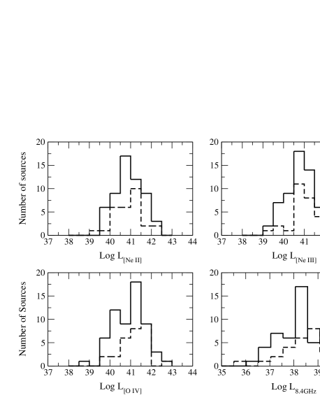
Figure 2: Comparison of the [Ne II], [Ne III], [O IV] and 8.4 GHz luminosities (in $ergs~{}s^{-1}$) in Seyfert 1 (dashed line) and Seyfert 2 (solid line) galaxies. This sample includes 29 Seyfert 1 galaxies and 59 Seyfert 2 galaxies for the mid-infrared luminosity distributions. Upper limits are not included in the 8.4 GHz luminosity distribution. The K-S test for these luminosities returns a $\sim 96.9\%$, $\sim 47.9\%$,$\sim 27.8\%$ and $\sim 82.0\%$ probability of the null hypothesis for the [Ne II], [Ne III], [O IV] and 8.4 GHz luminosities, respectively

It can be seen that Seyfert 1 and Seyfert 2 galaxies have similar distribution of values. As discussed in Meléndez et al. (2008b), there is an apparent lack of low luminosity Seyfert 1 galaxies in the [O IV] and [Ne III] distribution, but we find this difference not to be statistically significant, as shown by the K-S test results. Moreover, the sample presented in this work spans the same range on [O IV] luminosities as the revised Shapley-Ames sample (Diamond-Stanic et al., 2009). The good agreement between Seyfert 1 and Seyfert 2 galaxies in the radio continuum and mid-infrared emission line luminosity distributions demonstrates the isotropic properties of these quantities.

Table 3: Statistical Comparison Between Seyfert 1 and Seyfert 2 Galaxies

	Seyfert 1			Seyfert 2
	Measurements		Standard	Measurements		Standard	${\rm P_{K-S}}$
	Available	Median	Deviation	Available	Median	Deviation	(%)
Log 8.4GHz/[O IV]	27	-2.8	0.1	55	-2.6	0.1	8.2
Log 8.4GHz/[Ne III]	27	-2.6	0.1	55	-2.5	0.1	57.3
Log 8.4GHz/[Ne II]	27	-2.5	0.1	55	-2.6	0.1	81.6
${\rm L_{1.4GHz}}$	19	38.3	0.2	36	38.2	0.1	86.8
${\rm L_{8.4GHz}}$	27	38.4	0.2	55	38.4	0.1	82.0
${\rm L_{[OIV]}}$	29	41.3	0.1	59	41.0	0.1	27.8
${\rm L_{[NeIII]}}$	29	41.0	0.1	59	40.9	0.1	47.9
${\rm L_{[NeII]}}$	29	40.9	0.1	59	41.0	0.1	96.9

Note: The last column, ${\rm P_{K-S}}$, represents the Kolmogorov-Smirnov (K-S) test null probability. Upper limits for the 8.4 GHz fluxes are not included.

3 Mid-Infrared and the 8.4 GHz (3.6 cm) Emission

In order to understand the different contributions to the radio core emission and its interaction with the narrow-line region in Seyfert galaxies we investigated the mid-infrared emission line and 8.4 GHz correlations. One should note that, due to redshift effects, luminosity-luminosity plots will almost always show some correlation. Furthermore, caution must be taken when applying statistical analysis to data sets that contain non-detections (upper limits), or “censored” data points. In order to deal with these problems we used Astronomy SURVival analysis ASURV Rev 1.2 (Isobe & Feigelson, 1990; Lavalley et al., 1992), which implement the methods presented in Isobe et al. (1986). We also used a test for partial correlation with censored data (Akritas & Siebert, 1996) in order to exclude the redshift effect in the correlations. A detailed comparison between the correlation coefficient for different radio-to-mid-infrared correlations is presented in Table 4.

Table 4: Statistical Comparison of the Relationships Between Radio and Mid-Infrared Emission Lines Luminosities for the Sample

$\log-\log$	$\rho_{s}$	$P_{\rho}$	$\tau$	$P_{\tau}$	$\tau_{p}$	$\sigma$	$P_{\tau,p}$
All The Sample
8.4GHz-[O IV]	0.66	$<1\times 10^{-6}$	0.50	$<1\times 10^{-6}$	0.35	0.08	$<1\times 10^{-6}$
8.4GHz-[Ne III]	0.75	$<1\times 10^{-6}$	0.57	$<1\times 10^{-6}$	0.44	0.07	$<1\times 10^{-6}$
8.4GHz-[Ne II]	0.74	$<1\times 10^{-6}$	0.54	$<1\times 10^{-6}$	0.40	0.06	$<1\times 10^{-6}$
AGN Dominated Sources
8.4GHz-[O IV]	0.76	$<1\times 10^{-6}$	0.58	$<1\times 10^{-6}$	0.46	0.09	$<1\times 10^{-6}$
8.4GHz-[Ne III]	0.80	$<1\times 10^{-6}$	0.62	$<1\times 10^{-6}$	0.51	0.09	$<1\times 10^{-6}$
8.4GHz-[Ne II]	0.82	$<1\times 10^{-6}$	0.64	$<1\times 10^{-6}$	0.53	0.09	$<1\times 10^{-6}$
Star Formation Dominated Sources
8.4GHz-[O IV]	0.59	$1.30\times 10^{-3}$	0.42	$5.00\times 10^{-4}$	0.22	0.12	$6.23\times 10^{-2}$
8.4GHz-[Ne III]	0.68	$1.92\times 10^{-4}$	0.51	$2.80\times 10^{-5}$	0.32	0.12	$8.80\times 10^{-3}$
8.4GHz-[Ne II]	0.64	$5.00\times 10^{-4}$	0.47	$1.00\times 10^{-4}$	0.30	0.11	$6.60\times 10^{-3}$

Note: $\rho_{s}$ is the Spearman rank order correlation coefficient with its associated null probability, $P_{\rho}$. $\tau$ represents the generalized Kendall’s correlation coefficient for censored data and $\tau_{p}$ is the Kendall’s coefficient for partial correlation with censored data. $P_{\tau}$ and $P_{\tau,p}$ are the null probabilities for the generalized and partial Kendall’s correlation test, respectively. We also show the calculated variance, $\sigma$, for Kendall $\tau_{p}$. We have used a partial correlation test to exclude the effect of redshift (distance) in the luminosity-luminosity correlations.

We first considered the ratio between the radio continuum at 8.4 GHz ($L_{8.4GHz}$) and the [O IV] emission line. The K-S test for this ratio returns a $\sim 8.2\%$ probability of the null hypothesis (see Table 3). Therefore, the radio emission relative to the power of the AGN, as measured by the [O IV] emission, is statistically similar in both Seyfert 1 and Seyfert 2 galaxies, suggesting the isotropic property of the radio emission (e.g., Thean et al., 2001; Diamond-Stanic et al., 2009). This result is expected because the radio emission is expected to be unaffected by the torus. When using the generalized Spearman correlation test to compare this ratio with the [O IV] and 8.4 GHz luminosities we find no correlation with the [O IV] luminosities ($\rho_{s}=0.05;~{}P_{\rho}=0.64$) and a good correlation with the 8.GHz luminosity ($\rho_{s}=0.72;~{}P_{\rho}<1\times 10^{-6}$), see Figure 3. These results suggest that the radio loudness of the source cannot be associated solely with the strength of the AGN. In the following section we will elaborate on the implications of this result in view of the link between radio loudness and the mass accretion rates for the AGN. From the 8.4GHz/[Ne III] and 8.4GHz/[Ne II] ratios we found that Seyfert 1 and Seyfert 2 galaxies also have statistically similar distributions. The K-S test returns a 57.3$\%$ and 81.6$\%$ probability of the null hypothesis for the 8.4GHz/[Ne III] and 8.4GHz/[Ne II] ratios, respectively (see Table 3). The 8.4GHz-to-mid-infrared ratios are presented in Table 1.

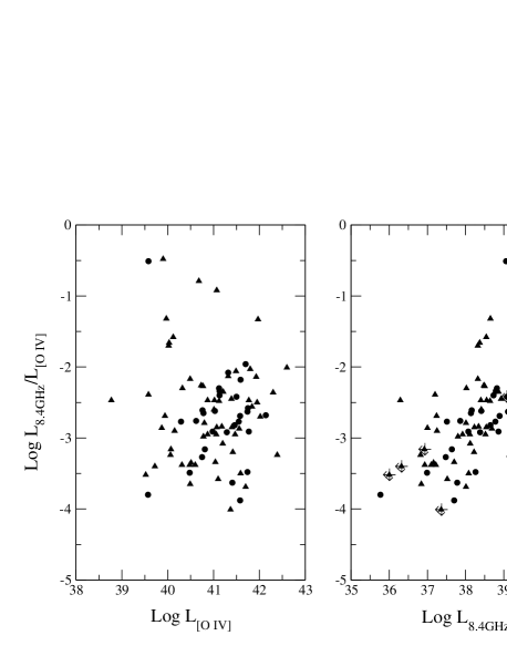
Figure 3: Correlation between the ratio $L_{8.4GHz}/L_{[OIV]}$ and the [O IV] and 8.4 GHz luminosities in Seyfert 1 (circles) and Seyfert 2 (triangles) galaxies.

Because Seyfert 1 and Seyfert 2 galaxies have statistically similar radio emission, relative to the strength of the AGN, we separated our sample in two new groups: 1) AGN and 2) star formation dominated sources, by following our previous study on the AGN and star formation contribution to the [Ne II] emission line (Meléndez et al., 2008b). In this new scheme, sources with more than 50$\%$ contribution from the AGN to the [Ne II] emission line are considered to be AGN dominated and sources with less than 50$\%$ contribution from the AGN to the [Ne II] emission line, or alternatively, more than 50$\%$ contribution from stellar activity to the [Ne II] emission are star formation dominated. One must note that in active galaxies with strong star formation, the [O IV] emission could be contaminated by the stellar activity, where the most likely contributor to the [O IV] emission is from HII regions ionized by Wolf-Rayet stars (see Hao et al., 2009, for discussion). However, if we correct the [O IV] emission for stellar contamination in star formation dominated sources, the resulting [O IV]/[Ne II] ratio will have even smaller values, thus reinforcing this quantitative classification. Moreover, sources that are well known to harbor massive star formation regions, such as NGC 3079 and NGC 6240 may have an additional complication because of contamination from the adjacent [Fe II] $\lambda$25.99$\mu{\rm m}$ line from the [O IV] in low-resolution IRS spectra. Following the discussion presented in Meléndez et al. (2008a) for NGC 3079, we estimated the starburst contribution to be $\sim 1.5$ times the uncontaminated [O IV] emission; similar results are obtained when comparing our fluxes with high-resolution spectroscopy for NGC 6240 (Armus et al., 2006). Nevertheless, these extreme cases have been classified correctly as star formation dominated sources. Moreover, a factor of $\sim 2$ in the [O IV] flux represents a dispersion of 0.3 dex, thus within the observed dispersion for the correlations presented in this study.

From this new classification we found that, star formation and AGN dominated sources are statistically different in their radio emission relative to the AGN. The K-S test for the 8.4GHz/[O IV] ratio returns a $\sim 0.1\%$ probability of the null hypothesis, i.e., indicating that star formation and AGN dominated galaxies are from different populations. Figure 4 shows the distribution of values for the $L_{8.4GHz}/L_{[OIV]}$ ratio for Seyfert 1 and Seyfert 2 galaxies, as well as for AGN and star formation dominated sources, where the differences in distributions can be clearly seen. On the other hand, the K-S test returns a 11.9$\%$ and 10.2$\%$ probability of the null hypothesis for the 8.4GHz/[Ne III] and 8.4GHz/[Ne II] ratios, respectively (see Table 4). Table 4 also includes information about the numbers of AGN and star formation dominated sources, median values and standard deviations of the mean for the measured quantities. One must note that a high stellar contribution to the [Ne II] emission, based on the [O IV]/[Ne II] ratio and typical of star formation dominated sources, does not always translate into higher SFRs, but could also indicate a relatively weak AGN (see Meléndez et al., 2008b).

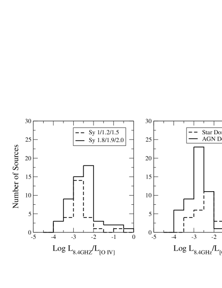
Figure 4: Comparison of the $L_{8.4GHz}/L_{[OIV]}$ ratio in Seyfert 1 and Seyfert 2 galaxies and AGN and star formation dominated sources. This sample includes 53 AGN dominated Seyfert galaxies and 29 star formation dominated sources for the distributions. Upper limits for the 8.4 GHz fluxes are not included. The K-S test for these ratios return $\sim 8.2\%$ and $\sim 0.1\%$ probability of the null hypothesis between Seyfert 1 and Seyfert 2 galaxies and AGN and star formation dominated galaxies, respectively

Table 5: Statistical Comparison Between AGN and Star Formation Dominated Sources

	AGN Dominated			STAR Dominated
	Measurements		Standard	Measurements		Standard	${\rm P_{K-S}}$
	Available	Median	Deviation	Available	Median	Deviation	(%)
Log 8.4GHz/[O IV]	53	-2.8	0.1	29	-2.4	0.1	0.3
Log 8.4GHz/[Ne III]	53	-2.7	0.1	29	-2.4	0.1	11.9
Log 8.4GHz/[Ne II]	53	-2.5	0.1	29	-2.7	0.1	10.2
Log 1.4GHz/[O IV]	27	-3.0	0.1	16	-2.5	0.1	0.2
Log 1.4GHz/[Ne III]	27	-2.8	0.1	16	-2.4	0.1	18.9
Log 1.4GHz/[Ne II]	27	-2.8	0.1	16	-2.9	0.1	12.3

Note: The last column, ${\rm P_{K-S}}$, represents the Kolmogorov-Smirnov (K-S) test null probability. Upper limits for the 8.4 GHz and 1.4 GHz fluxes are not included.

4 The Radio-to-Mid-Infrared radio loudness diagnostic

By looking at the mid-infrared and radio correlations in terms of the dominant source of the [Ne II] emission, we can investigate on the relationship between the radio emission and the nuclear activity. Figures 5-7 show the mid-infrared and 8.4 GHz luminosities with AGN and star formation dominated sources indicated. In particular, in the [O IV]-8.4 GHz correlation, Figure 5, the upper region of the plot ($>+\sigma$) contains only AGN dominated sources while star formation dominated sources tend to occupied the lower region ($<-\sigma$). Comparing Figures 5-7 one must note how the clear separation between the two groups is lost when decreasing the ionization potential of the emission lines or, alternatively, when the emission line has a stronger starburst component, in agreement with the K-S test results. For the star formation dominated region, the [O IV] underpredicts the observed 8.4 GHz emission. This suggest two possible scenarios: 1) star formation could enhance the 8.4 GHz emission and/or 2) the AGN in star formation dominated sources is more radio loud than estimated via standard radio-to-optical estimates.

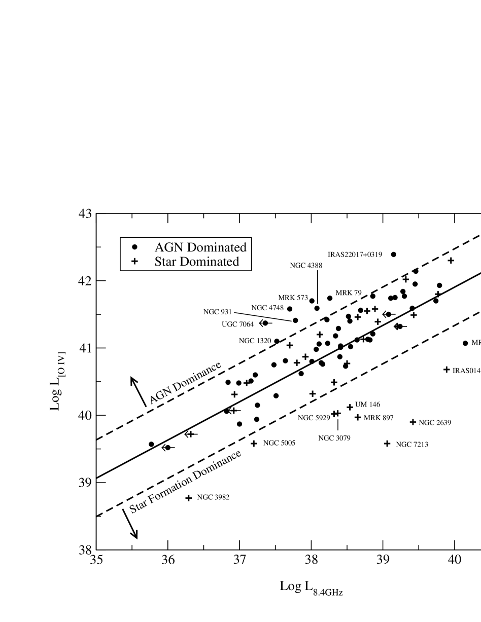
Figure 5: Correlation between the [O IV] and the 8.4 GHz emission. The circles represent the AGN dominated sources and the crosses represent the star formation dominated sources. The solid line represents the linear regression for the whole sample and the dashed lines represent a $1-\sigma$ dispersion.

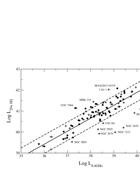
Figure 6: Correlation between the [Ne III] and the 8.4 GHz emission. The circles represent the AGN dominated sources and the crosses represent the star formation dominated sources. The solid line represents the linear regression for the whole sample and the dashed lines represent a $1-\sigma$ dispersion

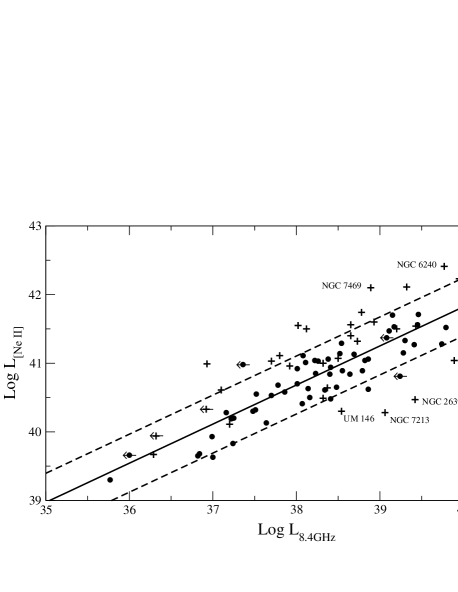
Figure 7: Correlation between the [Ne II] and the 8.4 GHz emission.The circles represent the AGN dominated sources and the crosses represent the star formation dominated sources. The solid line represents the linear regression for the whole sample and the dashed lines represent a $1-\sigma$ dispersion

In order to determine if star formation activity may contaminate the nuclear 8.4 GHz emission we proceed to estimate the 8.4 GHz emission associated with the star formation rates (SFR). For the SFR we adopted the values derived from the stellar component of the [Ne II] emission (Meléndez et al., 2008b). Then we used the calibration found by Schmitt et al. (2006) between the SFR and the 8.4 GHz emission. This calibration includes both the thermal and non-thermal SFR radio contribution (see Table 6). From this we found that the SFR overpredicts the observed 8.4 GHz luminosities in NGC 3982, NGC 5005 and MRK 897. This result is expected because the VLA in A configuration at 8.4 GHz sample a more compact region than that from the short-low and short-high resolution Spitzer slits, from which we extracted the [Ne II] emission. Therefore, the 8.4 GHz emission derived from the [Ne II] SFRs, represents an upper limit for the star formation contribution, if any, to the radio emission at 8.4 GHz. On the other hand, the SFR underpredicts the 8.4 GHz emission for 6 out of 9 of the sources in the star formation dominated region. For these six sources, stellar activity cannot be solely responsible for the observed radio excess because it can only account for a contribution as little as $\sim 2\%$ and no greater than $\sim 40\%$ of the observed flux, even when including the radio contribution from the extended star formation associated with the [Ne II] emission. One must note that the estimated SFRs represent a lower-limit as we neglect the stellar [Ne III] contribution (see Meléndez et al., 2008b, for discussion). However, all these sources have weak [Ne III], compared to the [Ne II] emission, hence the SFR will not be significantly affected nor the estimates for the radio emission.

Table 6: Comparison between the observed and predicted 8.4 GHz luminosities for the sources in the star formation dominated region

Name	Obs.	Pred.(SFR)
	Luminosity (${\rm W~{}Hz^{-1}}$)
IRAS01475-0740	22.96	21.38
MRK 897	21.73	22.02
NGC 2639	22.50	20.83
NGC 3079	21.44	21.02
NGC 3982	19.37	20.06
NGC 5005	20.27	20.44
NGC 5929	21.40	20.84
NGC 7213	22.14	20.66
UM 146	21.61	20.49

Note: In order to estimate the predicted 8.4 GHz luminosities we used the SFR values derived from the stellar component of the [Ne II] emission (Meléndez et al., 2008b). We adopted the calibration found by Schmitt et al. (2006) between the SFR and the 8.4 GHz emission.

Ho (2002) found an intriguing anticorrelation between the radio loudness of the galaxies, given by the radio-to-optical parameter, and the Eddington ratios, ${\rm L_{bol}/L_{Edd}}$, where $L_{bol}$ is the bolometric luminosity and $L_{Edd}$ is the Eddington luminosity. In general he found that galaxies with Eddington ratios $<10^{-5}$ are in the radio loud territory, while galaxies with Eddington ratios of $>1$ are in the radio quiet regime. In order to investigate this dichotomy we first need to estimate ${\rm L_{bol}}$. Heckman et al. (2004) first suggested that the luminosity of [O III] 5007Å  can be use as a proxy for the bolometric luminosity. In this regard, and by extending this analysis into the mid-infrared, Dasyra et al. (2008) found that ${\rm L_{[O~{}IV]}}$ is related to the 5100Å   continuum luminosity for a sample of reverberation-mapped AGN. From this and by using an estimate for the correction between the bolometric luminosity and the optical luminosity, ${\rm L_{bol}\approx 9\lambda L_{\lambda}(5100)}$ (Kaspi et al., 2000), they determined a scaling factor of 4500 between ${\rm L_{bol}}$ and ${\rm L_{[O~{}IV]}}$ with a variance of 0.5 dex. Because [O IV] is less sensitive to reddening corrections and is less contaminated by star-forming regions, by using ${\rm L_{[O~{}IV]}}$ as a bolometric luminosity indicator we can avoid the limitations of the ${\rm L_{[O~{}III]}}$ method. However, caution must be taken as for any of these methods the assumption is that the luminosity from narrow emission lines represents the same fraction of ${\rm L_{bol}}$ for all AGN. Moreover, the bolometric correction could be a function of the source luminosity and/or redshift (Netzer et al., 2006).

In order to calculate the Eddington luminosity we searched the literature for black hole (BH) masses, and found 81 BH masses for our radio sample. For the sake of uniformity, most of the values for the BH masses were calculated by using the relationship between the black hole mass and the stellar velocity dispersion found by Tremaine et al. (2002), except when noted in Table 1. Previous studies have suggested an uncertainty of 0.3 dex for the BH masses (e.g., Ho, 2002), however a more conservative uncertainty of 0.5 dex may be more appropriate for relatively low mass BH ($M_{BH}<10^{7}M_{\odot}$). One must note that the range for the normalized accretion rate, ${\rm L_{bol}/L_{Edd}}$, in our sample is in agreement with the range of values found for the radio quiet sources presented in Ho (2002). The Eddington ratios, ${\rm L_{bol}/L_{Edd}}$, are presented in Table 1.

In Figure 8 we show that a number of star formation dominated sources have smaller Eddington ratios in agreement with the radio excess observed in the star formation dominated region in the [O IV]-8.4 GHz correlation. There is certainly a trend of the Eddington ratios decreasing with increase radio loudness for star formation dominated sources, but this correlation is not statistically significant with this trend been dominated by the sources in the star formation dominated region. Also, there is an inherent scatter because of the uncertainties in the BH mass estimate. Nevertheless, these results show that star formation dominated sources with the bigger radio contribution, i.e., sources in the star formation dominated region, have smaller mass accretion rates. In this regard we also examined the dependence of the [O IV] luminosity on black hole mass (see Figure 9). From this comparison it can be seen that star formation dominated sources tend to have smaller accretion rates. Although the scatter is very large, there is a trend of $L_{[OIV]}$ increasing with $M_{BH}$.

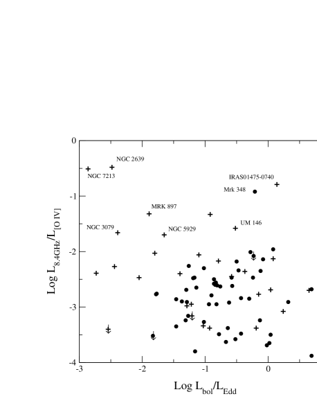
Figure 8: Comparison between ${\rm L_{bol}/L_{Edd}}$ and ${\rm L_{8.4GHz}/L_{[OIV]}}$ as a proxy for the AGN radio loudness. The symbols are the same as in Figure 5

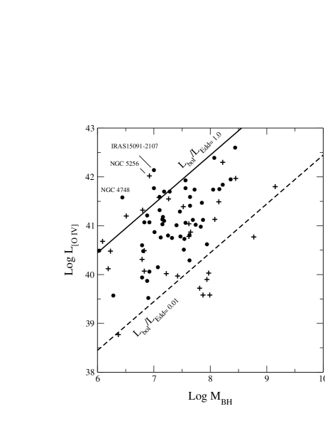
Figure 9: Dependence of [O IV] luminosity on black hole mass. The solid and dashed lines represent different values for Eddington accretion rates. The symbols are the same as in Figure 5

Using the radio-to-mid-infrared ratio, 8.4GHz/[O IV], we found that star formation dominated sources are, on average, $\sim 2.8$ times more radio loud than AGN dominated sources (see Table 5). This ratio has the advantage of classifying galaxy radio loudness without star formation contamination and/or dust extinction in the determination of the optical luminosity. On the other hand, the galaxy radio loudness determined from the 8.4GHz/[Ne III] and 8.4GHz/[Ne II] ratios could be a closer match to the historically radio loudness parameter, $R$, because these fine-structure lines of neon could be affected by star formation contamination, especially in weak or low-luminous AGN. Moreover, in some AGN, the observed [Ne V]14.32 $\micron$/[Ne V]24.32 $\micron$ ratio seems to fall below the low-density limit, implying a wavelength dependent extinction in the mid-infrared, with stronger extinction at shorter wavelengths (e.g., Dudik et al., 2007; Goulding & Alexander, 2009), suggesting that [Ne III] and [Ne II] could be more affected by dust extinction than [O IV], attributing the statistical differences between radio loudness in AGN and star formation dominated sources observed with these ratios.

Overall, we found a good correlation between all the mid-infrared lines and the 8.4 GHz luminosities in AGN dominated sources. On the other hand, the correlations for star dominated sources seems to be strongly affected by the distance as these correlations are not statistically significant when using a partial correlation test with the effect of redshift excluded (see Table 4). These results suggest that the nuclear 8.4 GHz radio emission cannot be associated directly with the intrinsic power of the AGN, as measured with [O IV], in sources that are dominated by star formation, or alternatively in low-luminosity AGN, nor can it be associated with star formation emission, because the SFRs for most of these sources underpredict the observed 8.4GHz luminosity (see Table 6). This may argue in favor of an advection dominated accretion flow (ADAF) model for the accretion disk (e.g., Narayan & Yi, 1994). In this model, the low accretion rates for the infalling material may never form a thin disk because of inefficient cooling, with the main coolant process being cyclo-synchrotron emission, which result in a compact radio emission source that is faint in other wavelengths, providing an alternative to low-power jets models in radio quiet sources. The accretion rates for some sources in the star formation dominated region are sufficiently sub-Eddington to support the ADAFs accretion models,e.g., low-luminous sources with a bright nuclear radio emission (see Table 1). Previous studies have suggested ADAF-type accretion flow models to explain the sub-Eddington accretion nature of two of the more extreme sources presented in this work, NGC 2639 and NGC 7213 (e.g., Terashima & Wilson, 2003; Starling et al., 2005). Our results support this scenario in light of the observed radio “excess”, compared to the intrinsic power of the AGN, as these are the most radio loud sources in our sample (see Table 1 and Figure 8). One may consider that star formation dominated sources could have a greater amount of fueling material in their nuclear regions, contrary to the ADAFs accretion models, but as we have mentioned before, sources with higher star formation contributions to [Ne II] do not necessarily have high SFR.

Figure 10: Correlation between the [O IV] and the 1.4 GHz emission. The red diamonds represent the AGN dominated sources and the blue squares represent the star formation dominated sources. The solid line represents the linear regression for the whole sample and the dashed lines represent a $1-\sigma$ dispersion

Finally, we compared the radio-to-mid-infrared parameter by using VLA B-configuration radio flux densities at 1.4 GHz and the mid-infrared emission lines, between AGN and star formation dominated sources. As we mentioned before, to estimate the radio contribution from the AGN one needs to use high angular resolution data, which are less contaminated by star formation from the host galaxy, except for the nuclear stellar activity. However, caution must been taken because at 1.4 GHz the region sampled by the VLA B-configuration could be contaminated by star formation in the circumnuclear region (within the inner few kpc). However, when comparing the shape of the SED between 1.4 GHz and 8.4 GHz emission we found that the K-S test for the spectral indices distribution, between AGN and star formation dominated sources, returns a $\sim 51.1\%$ probability of the null hypothesis. This result suggest that stellar activity is not the leading effect that drives the radio core correlation, as we found previously with the 8.4 GHz emission or, in other words, the high-resolution radio images at 1.4 GHz and 8.4 GHz are, on average, dominated by the active nuclei. Moreover, Meléndez et al. (2008a) suggested that because its high ionization potential the [O IV] emission is well within the Spitzer aperture on scales of less than a few hundreds of parsecs, typical of the NLR. From the 1.4GHz/[O IV] ratios we found that star formation and AGN dominated sources are statistically different in their radio loudness. The K-S test for this ratio returns a $\sim 0.2\%$ probability of the null hypothesis with star formation dominated sources more radio loud by a factor $\sim 3$ than AGN dominated sources, in close agreement with our previous finding using the radio core emission at 8.4 GHz. On the other hand, the K-S test returns a 18.9$\%$ and 12.3$\%$ probability of the null hypothesis for the 1.4GHz/[Ne III] and 1.4GHz/[Ne II] ratios, respectively (see Table 4). These results corroborate our assumption that the [O IV] emission is a true indicator of the AGN power, as the [Ne II] and [Ne III] emission could have a strong starburst component in weak AGN. Figure 10 shows the 1.4GHz-[O IV] correlation, where one can see the separation between AGN and star formation dominated sources, in agreement with the K-S test results and despite the smaller sample because of the limited number of high-resolution observations.

5 Conclusions

We have investigated the relationship between the radio emission and the ionization state of the emission-line gas in Seyfert galaxies with the aim to understand the connection between the radio loudness and the ionizing luminosities of the AGN. We used the [O IV] emission line to estimate the intrinsic power of the AGN and high-resolution 8.4 GHz emission to characterize the radio core power. From this we defined a radio-to-mid-infrared parameter, 8.4GHz/[O IV], to identify the radio contribution from the Seyfert nuclei. We found that Seyfert 1 and Seyfert 2 galaxies are statistically similar in their radio emission, relative to the strength of the AGN. On the other hand, when separated by the dominant source of [Ne II] emission, we found that two groups, AGN and star formation dominated sources, are statistically different in their radio loudness. We found that sources with strong star formation, relative to the strength of the AGN, or alternatively weak AGNs, tend to be more radio loud, by a factor of $\sim 2.8$, than AGN dominated sources. Furthermore, in the 8.4GHz-[O IV] correlation, sources in the star formation dominated region have lower mass accretion rates than the rest of the sample. This result is in agreement with the anticorrelation found by Ho (2002) between the radio loudness and Eddington accretion rates. Given the sub-Eddington nature of the more radio loud sources in our sample, sources in the star formation dominated region, one can invoke advection-dominated accretion models to explain their bright compact radio emission and a low-luminous nucleus both consistent with their high radio-to-mid-infrared parameter.

We also found that high resolution 1.4 GHz emission could also be used as a reasonable proxy for the AGN radio contribution. When using the 1.4GHz/[O IV] ratios we found that sources in which the [Ne II] emission is dominated by the stellar activity, or alternatively weak AGNs, tend to be more radio loud, by a factor of $\sim 3.0$, than AGN dominated sources, in close agreement with the radio loudness characterization using the radio core power at 8.4GHz. When comparing the observed 8.4 GHz and 1.4 GHz high-resolution core emission in our sample of Seyfert galaxies we found a strong linear correlation, suggesting that the core radio emission is dominated by the active nuclei with a spectral index of $f_{\nu}\propto\nu^{-0.7}$. We found the spectral index distribution, between 1.4 GHz and 8.4 GHz, for Seyfert 1 and Seyfert 2 galaxies and for AGN and star formation dominated sources to be statistically similar within the groups.

We suggest that the radio-to-optical parameter, $R$, used to classify galaxy radio loudness may erroneously quantize the radio contribution in galaxies with strong star formation or alternatively, weak AGNs, in which the optical luminosity may be contaminated by star formation and/or suffer from dust extinction. Instead, we found that a radio-to-mid-infrared parameter, 8.4GHz/[O IV], is a better probe for the radio loudness of the galaxy, as it is basically unaffected by star formation contamination and is less affected by extinction than optically dependent diagnostics.

Appendix A Spitzer/IRS Low-Resolution 5-35 $\mu$m Spectra of the Sample

The full sample presented in this work includes mid-infrared fluxes from Deo et al. (2007), Tommasin et al. (2008), Sturm et al. (2002), Weedman et al. (2005) and from our analysis of archival spectra observed with the Infrared Spectrograph (IRS) on board Spitzer Space Telescope (Werner et al., 2004). Figure 11 shows the resulting IRS low-resolution spectra (Short-Low, R$\sim$60$-$127 and Long-Low, R$\sim$57$-$126) from our analysis of archival spectra for 20 sources presented in the present work. The mid- and far-infrared properties of this sample are discussed in detail in Meléndez et al. (2008b). For the analysis of the mid-infrared spectra observed with IRS/Spitzer we followed the procedure described in Meléndez et al. (2008a).

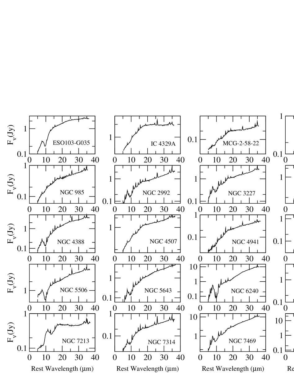
Figure 11: Spitzer/IRS low-resolution 5-35 $\mu$m spectra from our analysis of 20 sources presented in Meléndez et al. (2008b) and discussed in the present work

References

- Akritas & Siebert (1996) Akritas M. G., Siebert J., 1996, \mnras, 278, 919
- Antonucci (1993) Antonucci R., 1993, \araa, 31, 473
- Armus et al. (2006) Armus L., et al. 2006, \apj, 640, 204
- Baum et al. (1993) Baum S. A., O’Dea C. P., Dallacassa D., de Bruyn A. G., Pedlar A., 1993, \apj, 419, 553
- Becker et al. (1995) Becker R. H., White R. L., Helfand D. J., 1995, \apj, 450, 559
- Bevington & Robinson (2003) Bevington P. R., Robinson D. K., 2003, Data reduction and error analysis for the physical sciences. Data reduction and error analysis for the physical sciences, 3rd ed., by Philip R. Bevington, and Keith D. Robinson. Boston, MA: McGraw-Hill, ISBN 0-07-247227-8, 2003.
- Blundell & Beasley (1998) Blundell K. M., Beasley A. J., 1998, \mnras, 299, 165
- Buchanan et al. (2006) Buchanan C. L., et al. 2006, \aj, 132, 401
- Cid Fernandes et al. (2004) Cid Fernandes R., et al. 2004, \mnras, 355, 273
- Colbert et al. (1994) Colbert E. J. M., Wilson A. S., Bland-Hawthorn J., 1994, \apj, 436, 89
- Condon (1992) Condon J. J., 1992, \araa, 30, 575
- Condon & Broderick (1988) Condon J. J., Broderick J. J., 1988, \aj, 96, 30
- Condon et al. (1982) Condon J. J., Condon M. A., Gisler G., Puschell J. J., 1982, \apj, 252, 102
- Condon et al. (1987) Condon J. J., Gower A. C., Hutchings J. B., 1987, \aj, 93, 255
- Dahari & De Robertis (1988) Dahari O., De Robertis M. M., 1988, \apjs, 67, 249
- Dasyra et al. (2008) Dasyra K. M., et al. 2008, \apjl, 674, L9
- Davies et al. (1998) Davies R. E., et al. 1998, \mnras, 293, 189
- Deo et al. (2007) Deo R. P., Crenshaw D. M., Kraemer S. B., Dietrich M., Elitzur M., Teplitz H., Turner T. J., 2007, \apj, 671, 124
- Diamond-Stanic et al. (2009) Diamond-Stanic A. M., Rieke G. H., Rigby J. R., 2009, \apj, 698, 623
- Doyon et al. (1994) Doyon R., Wells M., Wright G. S., Joseph R. D., Nadeau D., James P. A., 1994, \apjl, 437, L23
- Dudik et al. (2009) Dudik R. P., Satyapal S., Marcu D., 2009, \apj, 691, 1501
- Dudik et al. (2007) Dudik R. P., Weingartner J. C., Satyapal S., Fischer J., Dudley C. C., O’Halloran B., 2007, \apj, 664, 71
- Garcia-Rissmann et al. (2005) Garcia-Rissmann A., Vega L. R., Asari N. V., Cid Fernandes R., Schmitt H., González Delgado R. M., Storchi-Bergmann T., 2005, \mnras, 359, 765
- González Delgado et al. (2001) González Delgado R. M., Heckman T., Leitherer C., 2001, \apj, 546, 845
- Goulding & Alexander (2009) Goulding A. D., Alexander D. M., 2009, \mnras, 398, 1165
- Greene & Ho (2007) Greene J. E., Ho L. C., 2007, \apj, 667, 131
- Greenhill et al. (2003) Greenhill L. J., et al. 2003, \apj, 590, 162
- Hao et al. (2009) Hao L., et al. 2009, \apj, 704, 1159
- Heckman et al. (2004) Heckman T. M., Kauffmann G., Brinchmann J., Charlot S., Tremonti C., White S. D. M., 2004, \apj, 613, 109
- Heisler et al. (1998) Heisler C. A., Norris R. P., Jauncey D. L., Reynolds J. E., King E. A., 1998, \mnras, 300, 1111
- Ho (2002) Ho L. C., 2002, \apj, 564, 120
- Ho (2007) Ho L. C., 2007, \apj, 668, 94
- Ho et al. (2009) Ho L. C., Greene J. E., Filippenko A. V., Sargent W. L. W., 2009, \apjs, 183, 1
- Ho & Keto (2007) Ho L. C., Keto E., 2007, \apj, 658, 314
- Ho & Peng (2001) Ho L. C., Peng C. Y., 2001, \apj, 555, 650
- Isobe & Feigelson (1990) Isobe T., Feigelson E. D., 1990, in Bulletin of the American Astronomical Society Vol. 22 of Bulletin of the American Astronomical Society, ASURV. The Pennsylvania State University. Report for the period Sep 1987 - Jan 1990.. pp 917–918
- Isobe et al. (1986) Isobe T., Feigelson E. D., Nelson P. I., 1986, \apj, 306, 490
- Kaspi et al. (2000) Kaspi S., Smith P. S., Netzer H., Maoz D., Jannuzi B. T., Giveon U., 2000, \apj, 533, 631
- Kawakatu et al. (2007) Kawakatu N., Imanishi M., Nagao T., 2007, \apj, 661, 660
- Kellermann et al. (1989) Kellermann K. I., Sramek R., Schmidt M., Shaffer D. B., Green R., 1989, \aj, 98, 1195
- Kirhakos & Steiner (1990) Kirhakos S. D., Steiner J. E., 1990, \aj, 99, 1722
- Kukula et al. (1995) Kukula M. J., Pedlar A., Baum S. A., O’Dea C. P., 1995, \mnras, 276, 1262
- Laine et al. (2006) Laine S., Kotilainen J. K., Reunanen J., Ryder S. D., Beck R., 2006, \aj, 131, 701
- Laor (2000) Laor A., 2000, \apjl, 543, L111
- Laor & Behar (2008) Laor A., Behar E., 2008, \mnras, 390, 847
- Lavalley et al. (1992) Lavalley M. P., Isobe T., Feigelson E. D., 1992, in Bulletin of the American Astronomical Society Vol. 24 of Bulletin of the American Astronomical Society, ASURV, Pennsylvania State University. Report for the period Jan 1990 - Feb 1992.. pp 839–840
- Lipari et al. (1991) Lipari S., Bonatto C., Pastoriza M. G., 1991, \mnras, 253, 19
- Maiolino et al. (1997) Maiolino R., Ruiz M., Rieke G. H., Papadopoulos P., 1997, \apj, 485, 552
- Markwardt et al. (2005) Markwardt C. B., Tueller J., Skinner G. K., Gehrels N., Barthelmy S. D., Mushotzky R. F., 2005, \apjl, 633, L77
- Meléndez et al. (2008a) Meléndez M., et al. 2008a, \apj
- Meléndez et al. (2008b) Meléndez M., Kraemer S. B., Schmitt H. R., Crenshaw D. M., Deo R. P., Mushotzky R. F., Bruhweiler F. C., 2008b, \apj
- Menon & Hickson (1985) Menon T. K., Hickson P., 1985, \apj, 296, 60
- Miller et al. (1990) Miller L., Peacock J. A., Mead A. R. G., 1990, \mnras, 244, 207
- Morganti et al. (1999) Morganti R., Tsvetanov Z. I., Gallimore J., Allen M. G., 1999, \aaps, 137, 457
- Morris et al. (1985) Morris S., Ward M., Whittle M., Wilson A. S., Taylor K., 1985, \mnras, 216, 193
- Nagar et al. (1999) Nagar N. M., Wilson A. S., Mulchaey J. S., Gallimore J. F., 1999, \apjs, 120, 209
- Narayan & Yi (1994) Narayan R., Yi I., 1994, \apjl, 428, L13
- Nelson & Whittle (1995) Nelson C. H., Whittle M., 1995, \apjs, 99, 67
- Netzer et al. (2006) Netzer H., Mainieri V., Rosati P., Trakhtenbrot B., 2006, \aap, 453, 525
- Ohta et al. (2007) Ohta K., Aoki K., Kawaguchi T., Kiuchi G., 2007, \apjs, 169, 1
- O’Neill et al. (2005) O’Neill P. M., Nandra K., Papadakis I. E., Turner T. J., 2005, \mnras, 358, 1405
- Peterson et al. (2004) Peterson B. M., et al. 2004, \apj, 613, 682
- Peterson & Wandel (2000) Peterson B. M., Wandel A., 2000, \apjl, 540, L13
- Press et al. (1992) Press W. H., Teukolsky S. A., Vetterling W. T., Flannery B. P., 1992, Numerical recipes in FORTRAN. The art of scientific computing. Cambridge: University Press, —c1992, 2nd ed.
- Rawlings et al. (1989) Rawlings S., Saunders R., Eales S. A., Mackay C. D., 1989, \mnras, 240, 701
- Rees (1984) Rees M. J., 1984, \araa, 22, 471
- Rigby et al. (2009) Rigby J. R., Diamond-Stanic A. M., Aniano G., 2009, \apj, 700, 1878
- Risaliti et al. (2009) Risaliti G., et al. 2009, \mnras, 393, L1
- Roy et al. (1994) Roy A. L., Norris R. P., Kesteven M. J., Troup E. R., Reynolds J. E., 1994, \apj, 432, 496
- Roy et al. (1998) Roy A. L., Norris R. P., Kesteven M. J., Troup E. R., Reynolds J. E., 1998, \mnras, 301, 1019
- Sanders et al. (1989) Sanders D. B., Phinney E. S., Neugebauer G., Soifer B. T., Matthews K., 1989, \apj, 347, 29
- Sandqvist et al. (1995) Sandqvist A., Joersaeter S., Lindblad P. O., 1995, \aap, 295, 585
- Schmitt et al. (2001) Schmitt H. R., Antonucci R. R. J., Ulvestad J. S., Kinney A. L., Clarke C. J., Pringle J. E., 2001, \apj, 555, 663
- Schmitt et al. (2006) Schmitt H. R., et al. 2006, \apj, 643, 173
- Starling et al. (2005) Starling R. L. C., Page M. J., Branduardi-Raymont G., Breeveld A. A., Soria R., Wu K., 2005, \mnras, 356, 727
- Sturm et al. (2002) Sturm E., et al. 2002, \aap, 393, 821
- Terashima & Wilson (2003) Terashima Y., Wilson A. S., 2003, \apj, 583, 145
- Thean et al. (2000) Thean A., Pedlar A., Kukula M. J., Baum S. A., O’Dea C. P., 2000, \mnras, 314, 573
- Thean et al. (2001) Thean A., Pedlar A., Kukula M. J., Baum S. A., O’Dea C. P., 2001, \mnras, 325, 737
- Thompson et al. (1980) Thompson A. R., Clark B. G., Wade C. M., Napier P. J., 1980, \apjs, 44, 151
- Tommasin et al. (2008) Tommasin S., Spinoglio L., Malkan M. A., Smith H., González-Alfonso E., Charmandaris V., 2008, \apj, 676, 836
- Tremaine et al. (2002) Tremaine S., et al. 2002, \apj, 574, 740
- Tueller et al. (2008) Tueller J., et al. 2008, \apj, 681, 113
- Ulvestad (1986) Ulvestad J. S., 1986, \apj, 310, 136
- Ulvestad et al. (1995) Ulvestad J. S., Antonucci R. R. J., Goodrich R. W., 1995, \aj, 109, 81
- Ulvestad & Wilson (1984a) Ulvestad J. S., Wilson A. S., 1984a, \apj, 278, 544
- Ulvestad & Wilson (1984b) Ulvestad J. S., Wilson A. S., 1984b, \apj, 285, 439
- Ulvestad & Wilson (1989) Ulvestad J. S., Wilson A. S., 1989, \apj, 343, 659
- Unger et al. (1987) Unger S. W., Lawrence A., Wilson A. S., Elvis M., Wright A. E., 1987, \mnras, 228, 521
- Visnovsky et al. (1992) Visnovsky K. L., Impey C. D., Foltz C. B., Hewett P. C., Weymann R. J., Morris S. L., 1992, \apj, 391, 560
- Wang et al. (2007) Wang J.-M., Chen Y.-M., Yan C.-S., Hu C., Bian W.-H., 2007, \apjl, 661, L143
- Weedman et al. (2005) Weedman D. W., et al. 2005, \apj, 633, 706
- Werner et al. (2004) Werner M. W., et al. 2004, \apjs, 154, 1
- Whittle (1992) Whittle M., 1992, \apjs, 79, 49
- Wu & Han (2001) Wu X.-B., Han J. L., 2001, \aap, 380, 31
- Xu et al. (1999) Xu C., Livio M., Baum S., 1999, \aj, 118, 1169
- Young et al. (1996) Young S., Hough J. H., Efstathiou A., Wills B. J., Bailey J. A., Ward M. J., Axon D. J., 1996, \mnras, 281, 1206