CCTP-2010-17 Classical ultrarelativistic bremsstrahlung in extra dimensions

Abstract

The emitted energy and the cross-section of classical scalar bremsstrahlung in massive particle collisions in $D=4+d-$dimensional Minkowski space ${\mathcal{M}}_{D}$ as well as in the brane world ${\mathcal{M}}_{4}\times{\mathcal{T}}^{d}$ is computed to leading ultra-relativistic order. The particles are taken to interact in the first case via the exchange of a bulk massless scalar field $\Phi$ and in the second with an additional massless scalar $\phi$ confined together with the particles on the brane. Energy is emitted as $\Phi$ radiation in the bulk and/or $\phi$ radiation on the brane. In contrast to the quantum Born approximation, the classical result is unambiguous and valid in a kinematical region which is also specified. For $D=4$ the results are in agreement with corresponding expressions in classical electrodynamics.

I Introduction and results

There is little doubt that new physics will soon be discovered at the TeV scale. Absence of a light fundamental higgs boson implies new physics and, furthermore, a light higgs boson is unstable without new physics, of which examples are supersymmetry broken at the TeV scale, or maybe some variant of gauge interaction becoming strong at the TeV scale iliopoulos .

A less well founded, but arguably more fascinating scenario for LHC would be the discovery of TeV scale gravity and Large Extra Dimensions (LEDs) ADD . Although extra dimensions were proposed a century ago, their raison d’ être, as well as their number, size and topology vary in different proposals. The potentially most natural justification of the existence of extra dimensions with a definite proposal for their number is string theory, while their most natural size is thought to be the Planck length $\mathcal{O}(10^{-16}\;{\rm TeV}^{-1})$. Nevertheless, the idea that some extra dimensions could be of order $\mathcal{O}({\rm TeV}^{-1})$ appeared in the context of heterotic string theory, when the size of extra dimensions was connected to the supersymmetry breaking scale ablt . Earlier thoughts of the Universe as a topological defect embedded in a higher-dimensional space-time defect and the development of the Brane-World idea led to a variety of alternative scenaria RS ; UED reviewed in reviews . They differ in the topology, size and geometry of the extra dimensions, as well as in the nature of the degrees of freedom which may propagate in the bulk. The technically simplest such model is the ADD ADD ; GRW , with the Standard Model particles confined on the brane and only gravity allowed to propagate in the whole ${\mathcal{M}}_{4}\times{\mathcal{T}}^{d}$ space-time.

The invention of ways to detect and measure the size of extra dimensions has attracted considerable attention and the study of radiation is an obvious candidate. Indeed, it has been argued that in the ADD model graviton bremsstrahlung from neutron collisions may give significant contribution to the cooling of supernovae bremnr , thus providing strong bounds on relevant parameters. Also, production of Kaluza-Klein (KK) gravitons in collisions of relativistic particles at LEP or LHC was extensively discussed in the literature, with emphasis on processes efficient to at least demonstrate their very existence MPP ; Dvergsnes:2002nc . However, the actual quantum perturbative calculations in the context of ADD are ambiguous, as they are plugged with tree-level divergences, associated with the emission of infinite momentum of modes into the compact dimensions GRW . This problem is manifest already in the calculation of any elastic scattering amplitude in such spaces and was treated in rather ad-hoc ways. Contrary to the above situation, a purely classical computation, which by itself carries a natural mechanism to cut-off the energetic KK excitations, leads to unambiguous results gkst . Theoretically, such an approach is justified by the fact that at transplanckian energies scattering processes are dominated by gravity, which in addition, may be treated classically, at least in some range of momentum transfer thooft . Furthermore, the classical formula for the elastic scattering in ADD was shown to coincide with the one obtained in the non-perturbative eikonal approximation, given by the summation of an infinite number of ladder graphs in quantum theory gkst .

Encouraged by the above result, one may try to deal in the same way with the phenomenon of ultra-relativistic gravitational bremsstrahlung, and the present paper is a first step in this direction. To further motivate this approach, it is well known that in 4-dimensions the classical treatment of relativistic bremsstrahlung corresponds to non-perturbative calculations in quantum electrodynamics. Specifically, bremsstrahlung in ultra-relativistic scattering off a Coulomb center has been computed using the exact Coulomb solutions of the Dirac equation (see bere and references therein). In the ultra-relativistic limit and with momentum transfer not exceeding the particle mass, a good approximation to the corresponding cross-section is given by the simplified Furry-Sommerfeld-Maue formula, which for photon energy much smaller than $E^{2}/m$, where $E$ and $m$ are the particle energy and mass respectively, reduces to the classical result GaGra . The result is clearly non-perturbative in the normal sense of expansion in powers of the fine structure constant. No analogous non-perturbative quantum calculations are available for bremsstrahlung in higher dimensions, especially in the presence of compact LEDs. Although certain aspects of classical radiation in $D-$dimensional Minkowski space were discussed recently minkd ; minkd1 , radiation in the presence of compact LEDs has not been considered so far. So, the hereby proposed classical treatment, which as explained in gkst is unambiguous and expected to be trustable in the ultra-relativistic limit and small scattering angle, is also, to the best of our knowledge, the first actual computation of the phenomenon in higher dimensional space-times with the topology of ${\mathcal{M}}_{4}\times{\mathcal{T}}^{d}$.

The purpose of this paper is to present a classical computation of bremsstrahlung in particle collisions on a flat 3-brane embedded in flat space-time of arbitrary dimension and with the transverse space taken either euclidean $\mathcal{E}^{d}$ (relevant to the scenario of Universal Extra Dimensions UED ) or toroidal ${\mathcal{T}}^{d}$ (as in ADD) with equal radii. As a first step, the bulk interaction will be modeled by the exchange of a massless scalar field $\Phi$, while an additional massless scalar $\phi$, confined on the brane, will be introduced to mimic, in the case of toroidal extra dimensions, the Standard Model interactions between the colliding particles. The case of gravity differs, of course, crucially from massless scalar exchange. Nevertheless, the present analysis captures several important technical points of gravitational bremsstrahlung gkst3 , to be presented in full detail elsewhere gkst4 .

Straightforward classical perturbation theory, developed in Section II, is applied to iteratively solve the particle equations of motion and the field equations as well. The radiation efficiency $\varepsilon$, i.e. the fraction of the initial energy emitted as bremsstrahlung radiation, is computed in Section II to leading ultra-relativistic order and low momentum transfer and is found to be

$$\varepsilon_{d}\equiv\frac{E_{\mathrm{rad}}}{E}\simeq{\mathcal{C}}_{d}\,(\gamma\,r_{d}^{3}/b^{3})^{1+d}\,,$$ (I.1)

where $r_{d}$ is the $D-$dimensional classical radius of the colliding particles and $b$ the impact parameter. The constant ${\mathcal{C}}_{d}$ is given in (II.47).

The case of toroidal extra dimensions is dealt with in Section III. The light $\Phi-$KK modes participate crucially both in the interaction between the colliding particles and in the radiation emitted in the bulk. These roles are studied separately with appropriate choices of their couplings to the radiating particles. The radiation efficiency, depending on which interaction is assumed to be dominant (via $\Phi$ or $\phi$) and on the nature of radiation ($\Phi-$radiation in the bulk or $\phi$ on the brane), is to leading ultra-relativistic order shown in Table 1. Note the interrelations among the various entries of the Table as well as with (I.1). The range of validity of the computation, the consequences of the results and the modifications expected in actual gravity are presented in the discussion Section IV gkst4 . Finally, three Appendices in the end contain derivations of formulas used and clarifications of technical approximations made in the text. They also contain a qualitative explanation of the basic features of Table I.

Radiation	Bulk ${\mathcal{M}}_{4}\times{\mathcal{T}}^{d}$	Brane ${\mathcal{M}}_{4}$
Interaction
Bulk ${\mathcal{M}}_{4}\times{\mathcal{T}}^{d}$	$\;\;\;\;\;\;\;\varepsilon_{\Phi\Phi}\simeq{\mathcal{C}}_{d}\,(\gamma\,r_{d}^{3}/b^{3})^{1+d}\;\;\;\;\;\;\;$	$\;\;\;\;\;\;\varepsilon_{\Phi\phi}\simeq{\mathcal{C}}_{\Phi\phi}\,\gamma\,\frac{R_{0}}{b}\,(\frac{r_{d}}{b})^{2(1+d)}\;\;\;\;\;\;$
Brane ${\mathcal{M}}_{4}$	$\varepsilon_{\phi\Phi}\simeq{\mathcal{C}}_{\phi\Phi}\,\left(\frac{R_{0}}{b}\right)^{2}\left(\gamma\,\frac{r_{d}}{b}\right)^{1+d}$	$\;\;\;\varepsilon_{\phi\phi}\simeq{\mathcal{C}}_{0}\,\gamma\,R_{0}^{3}/b^{3}\;\;\;$

Table 1: Radiation emission efficiency in ${\mathcal{M}}_{4}\times{\mathcal{T}}^{d}$. The standard “electromagnetic” ($R_{0}$) and the $D-$dimensional “gravitational” ($r_{d}$) classical radii of the colliding particles, as well as the constants ${\mathcal{C}}_{ab}$ and ${\mathcal{C}}_{0}$ are given in the text.

II Scalar ultra-relativistic bremsstrahlung in ${\mathcal{M}}_{D}$

In this section we formulate our approach in the simplest case of two massive scalar point charges interacting via a linear scalar field in Minkowski space of arbitrary dimension $D$. This will serve as a reference calculation for the subsequent treatment of compactified extra dimensions.

II.1 The model - Generalities

Consider two particles with masses $m$ and $m^{\prime}$ moving along the world-lines $x^{M}=z^{M}(\tau),\,x^{M}=z^{\prime M}(\tau^{\prime})$ interacting with a massless scalar field $\Phi$ with coupling constants $f$ and $f^{\prime}$, respectively. The relevant action is

$$S=-\int d\tau\sqrt{\dot{z}^{2}}[m+f\Phi(z)]-\int d\tau^{\prime}\sqrt{\dot{z}^{{}^{\prime}2}}[m^{\prime}+f^{\prime}\Phi(z^{\prime})]+\frac{1}{2}\int d^{D}x\partial_{M}\Phi\,\partial^{M}\Phi,\,$$ (II.1)

with $M,A,B,\ldots=0,1,\ldots,D-1=3+d$, and the metric signature is $(+,-,-,\ldots,-)$. $\dot{z}^{2}\equiv\eta_{MN}\dot{z}^{M}\dot{z}^{N}$, and the dot denotes differentiation with respect to $\tau$ or $\tau^{\prime}$. The classical radius $r_{d}$ of the particle $m$ is defined by

$$\frac{f^{2}}{m}\equiv r_{d}^{d+1}\,,$$ (II.2)

and similarly for $m^{\prime}$.

Linearity of the field equations implies that $\Phi=\Phi_{m}+\Phi_{m^{\prime}}$, where

$$\Box\,\Phi_{m}(x)=\rho(x),\quad\Box\,\Phi_{m^{\prime}}=\rho^{\prime}(x),\quad\Box\equiv\eta^{MN}\partial_{M}\partial_{N},$$ (II.3)

the sources being

$$\rho(x)=f\int d\tau\sqrt{\dot{z}^{2}}\delta^{D}(x-z(\tau)),\quad\rho^{\prime}(x)=f^{\prime}\int d\tau^{\prime}\sqrt{\dot{z}^{\prime 2}}\delta^{D}(x-z^{\prime}(\tau^{\prime})).$$ (II.4)

The particles’ equations of motion read

$$\frac{d}{d\tau}\left[(m+f\Phi)\dot{z}^{M}\right]=f\partial^{M}\Phi,$$ (II.5)

and similarly for $m^{\prime}$, provided the parameters $\tau,\tau^{\prime}$ are chosen so that

$$\dot{z}(\tau)^{2}=1=\dot{z}^{\prime}(\tau^{\prime})^{2}.$$ (II.6)

This can be rewritten as

$$(m+f\Phi)\ddot{z}^{M}=f\,\Pi^{MN}\partial_{N}\Phi,\quad\Pi^{MN}=\eta^{MN}-\dot{z}^{M}\dot{z}^{N},$$ (II.7)

where $\Pi^{MN}$ is the projector onto the space orthogonal to the world-line. In this equation the field on the right hand side contains both the self-action term ($\Phi_{m}$), and the mutual interaction term $\Phi_{m^{\prime}}$. The first gives rise to divergences, taken care of by mass renormalization, and also for $D\geqslant 4$ to the introduction of higher derivative classical counter-terms minkd , which for simplicity will be ignored. Thus, the equations of motion become:

$$(m+f\Phi_{m})\ddot{z}^{M}=f\Pi^{MN}\partial_{N}\Phi_{m^{\prime}},\quad(m^{\prime}+f^{\prime}\Phi_{m^{\prime}})\ddot{z}^{\prime M}=f^{\prime}\,\Pi^{\prime MN}\partial_{N}\Phi_{m}.$$ (II.8)

Fourier transform using $\Psi(x)\equiv\int\Psi(k){\rm e}^{-ik\cdot x}d^{D}k/(2\pi)^{D}$ and $\Psi(k)\equiv\int\Psi(x){\rm e}^{ik\cdot x}d^{D}x$. The retarded solutions of the wave equations (II.3) can then be written algebraically:

$$\Phi(k)=G_{\rm ret}(k)\rho(k),\quad G_{\rm ret}(k)=\bar{G}(k)+i\pi\varepsilon(k^{0})\delta(k^{2}),\quad\bar{G}(k)=-\;\mathcal{P}\frac{{1}}{k^{2}},$$ (II.9)

with the Fourier-transforms of the source terms given by:

$$\rho(k)=f\int{\rm e}^{ik\cdot z(\tau)}d\tau,\quad\rho^{\prime}(k)=f^{\prime}\int{\rm e}^{ik\cdot z^{\prime}(\tau^{\prime})}d\tau^{\prime}.$$ (II.10)

The energy-momentum $P^{M}$ of the scalar radiation, emitted by the particles during the scattering process, can be computed by integrating the field stress-tensor

$$T^{MN}=\partial^{M}\Phi\,\partial^{N}\Phi-\frac{1}{2}\eta^{MN}\partial_{L}\Phi\,\partial^{L}\Phi$$ (II.11)

between the space-like hypersurfaces $\Sigma_{\pm\infty}$ corresponding to $t\to\pm\infty$ and reads:

$$P^{M}=\int\limits_{\Sigma_{\infty}}T^{MN}dS_{N}-\int\limits_{\Sigma_{-\infty}}T^{MN}dS_{N}.$$ (II.12)

Given the fall-off of the stress-tensor at spatial infinity $T^{MN}\sim 1/r^{D-2}+\mathcal{O}(r^{-(D-1)})$ (derived from the behavior of the Liénard-Wiechert potentials), one can write $P^{M}$ as an integral over the closed boundary of the space-time tube and, subsequently, transform it to the volume integral $P^{M}=\int d^{D}x\nabla_{N}T^{MN}$, which upon substitution of (II.11) leads to

$$P^{M}=\int d^{D}x(\rho+\rho^{\prime})\;\partial^{M}\Phi,$$ (II.13)

or equivalently

$$P^{M}=-\frac{i}{(2\pi)^{D}}\int d^{D}k\,k^{M}\,\Phi(k)\left[\rho^{*}(k)+\rho^{\prime*}(k)\right].$$ (II.14)

Substituting here the retarded solution (II.9) and taking into account that the contribution of the principal part $\bar{G}(k)=-\;{\mathcal{P}}\,(k^{2})^{-1}$ vanishes being odd under $k^{M}\to-k^{M}$, one is led to

$$P^{M}=\frac{1}{(2\pi)^{D-1}}\int d^{D}k\,\theta(k^{0})k^{M}\delta(k^{2})|\rho(k)+\rho^{\prime}(k)|^{2}.$$ (II.15)

Finally, denote the frequency $k^{0}\equiv\omega$, use $\theta(k^{0})\delta(k^{2})=\delta(\omega-|\mathbf{k}|)/2|\mathbf{k}|$, and integrate over $|\mathbf{k}|$ to obtain the spectral-angular distribution of radiation:

$$\frac{dP^{M}}{d\omega d\Omega}=\frac{1}{2(2\pi)^{D-1}}\omega^{D-3}k^{M}|\rho(k)+\rho^{\prime}(k)|^{2}\Big{|}_{k^{M}=\omega(1,\mathbf{n})},$$ (II.16)

where $\Omega$ or $\mathbf{n}$ parametrize the unit sphere in the $(D-1)-$dimensional Euclidean subspace.

II.2 Perturbative solution

II.2.1 Particle trajectories

We next solve the equations of motion for the particles and the field $\Phi$ iteratively in powers of the coupling constants $f$ and $f^{\prime}$. For the particle trajectories we write

$$z^{M}(\tau)=b^{M}+u^{M}\tau+\delta z^{M}(\tau),\quad z^{\prime M}(\tau)=u^{\prime M}\tau+\delta z^{\prime M}(\tau),$$ (II.17)

(assuming $z^{M}(0)=b^{M},z^{\prime M}(0)=0$) where $u^{M}$ and $u^{\prime M}$ are the unperturbed constant four-velocities, specified by the initial condition and chosen to satisfy $u^{2}=1=u^{\prime 2}$. Combine with (II.6) to conclude that the perturbations of velocities must be orthogonal to the unperturbed world lines:

$$u_{A}\,\frac{d}{d\tau}(\delta z^{A})=0\;,\qquad u^{\prime}_{A}\,\frac{d}{d\tau^{\prime}}(\delta{z^{\prime}}^{A})=0\;.$$ (II.18)

To zeroth order, the solution of the wave equation describes the non-radiative Coulomb field of two non-interacting particles, which in terms of the Fourier-transform reads

$$\Phi_{m}(q)=-\frac{2\pi f}{q^{2}}{\rm e}^{iq\cdot z(0)}\delta(q\cdot u).$$ (II.19)

Substituting this into the equations of motion (II.8) we find for the first order perturbation:

$$\frac{d^{2}}{d\tau^{2}}{z}^{A}(\tau)=\frac{f}{m}\Pi^{AB}\partial_{B}\Phi_{m^{\prime}}(x)\Big{|}_{x^{A}=z^{A}(\tau)},$$ (II.20)

where $\Pi^{AB}=\eta^{AB}-u^{A}u^{B}$ is the projector on its unperturbed world-line. The solution for $\delta z$ is

$$\delta z^{M}(\tau)=-i\frac{ff^{\prime}}{m(2\pi)^{D-1}}\int\frac{d^{D}q}{q^{2}(q\cdot u)^{2}}{\rm e}^{-iq\cdot b}\left({\rm e}^{-i(q\cdot u)\tau}-1+iq\cdot u\tau\right)\delta(q\cdot u^{\prime})\Pi^{MN}q_{N}\,,$$ (II.21)

with an analogous expression for $\delta z^{\prime}$ and with the exchange $u\leftrightarrow u^{\prime},b\to-b$. They automatically satisfy the orthogonality conditions (II.18).

II.2.2 The radiation and its main features

The next step is to compute corrections to the field $\Phi$ due to these perturbations of the trajectories. These will correspond to the lowest order radiation field. To compute radiation using (II.16) one needs the Fourier transform of the corresponding sources. Our treatment is symmetric in $m$ and $m^{\prime}$, so we write only unprimed quantities. The zeroth order terms do not contribute to radiation, since the corresponding Fourier transforms (II.19) vanish on the light cone $k^{2}=0$ (except for the trivial point $k^{\mu}=0$). Ditto for the last two terms inside the parenthesis in the integrand of (II.21). Thus, to lowest non-trivial order :

$$\rho(k)\simeq if\int d\tau\,{\rm e}^{ik\cdot z(0)+i(k\cdot u)\tau}(k\cdot\delta z(\tau)).$$ (II.22)

Substitution of (II.21) gives

$$\rho(k)\simeq\frac{f^{2}f^{\prime}}{(2\pi)^{D-2}}\frac{\Pi_{MN}k^{M}I^{N}{\rm e}^{ik\cdot z(0)}}{m(k\cdot u)^{2}},$$ (II.23)

with

$$I^{M}(k)\equiv\int d^{D}q\frac{\delta(q\cdot u^{\prime})\delta((k-q)\cdot u)\,{\rm e}^{-iq\cdot b}}{q^{2}}q^{M}.$$ (II.24)

The corresponding integral $I^{\prime}_{A}(k)$ for the partner particle is obtained from $I_{A}$ by the substitution $u\leftrightarrow u^{\prime},z_{A}(0)\leftrightarrow z^{\prime}_{A}(0)$, $b_{A}\to-b_{A}$. The integrals are evaluated in Appendix I in a fully covariant form.

It is convenient to work in the lab frame, in which $u^{\prime A}=(1,0,0,...,0)$, i.e. with $m^{\prime}$ initially at rest. Define the remaining kinematical variables in this frame by

$$u^{A}=\gamma(1,{\bf{v}}),\;\;k^{A}=\omega(1,{\bf{n}}),\;\;k\cdot u=\gamma\omega\xi,\;\;\xi\equiv 1-v\cos\theta,\;\;k\cdot u^{\prime}=\omega,$$ (II.25)

where as usual $\gamma=1/\sqrt{1-v^{2}}$ and $\theta$ is the angle between $\bf{n}$ and $\bf{v}$. The invariant expression for the Lorentz factor is $\gamma=u\cdot u^{\prime}$.

Furthermore, we define the zeroes of the parameters $\tau$ and $\tau^{\prime}$ in such a way that at the point of closest proximity of the scattered particles they satisfy $u\cdot b=0={u^{\prime}}\cdot b$. In other words, the“initial conditions” defined at $\tau=0=\tau^{\prime}$ are given at the moment of least distance between the particles. But then, $b^{0}=0$ and $\mathbf{v}\cdot\mathbf{b}=0$ (easiest visualized in the CM frame). The vectors $\bf{v}$ and $\mathbf{b}$ define the collision plane, while the generic $(D-1)$-dimensional unit vector ${\bf n}$ can be decomposed as:

$$\bf{n}=\frac{\bf{v}}{|\bf{v}|}\cos\theta+\frac{\mathbf{b}}{|\mathbf{b}|}\sin\theta\sin\psi+\bf{m}\sin\theta\cos\psi,$$ (II.26)

where $\bf{m}$ is a $D-1$ dimensional unit vector orthogonal to the collision plane. Then

$${\bf{k}}\cdot{\mathbf{b}}=-k\cdot b=b\,\omega\sin\theta\sin\psi,$$ (II.27)

where the impact parameter $b\equiv|\mathbf{\Delta}|$ is also given by the invariant expression:

$$b=|\mathbf{b}|=\left(-b^{2}-\frac{[(u^{\prime}\cdot b)u-(u\cdot b)u^{\prime}]^{2}}{(u\cdot u^{\prime})^{2}v^{2}}\right)^{1/2}.$$ (II.28)

Occasionally, it will be convenient to express the angular dependence of radiation in the rest frame of the moving particle $m$. In that frame the radiation angle will be denoted by $\theta_{0}$, which is related to $\theta$ via

$$\cos\theta_{0}=\frac{1}{v}\left(\frac{1}{\xi\gamma^{2}}-1\right),\quad\sin\theta_{0}=\frac{\sin\theta}{\xi\gamma}.$$ (II.29)

Using formula (V.12) of Appendix I one obtains

$$\rho(k)\simeq\frac{f^{2}f^{\prime}e^{ik\cdot z(0)}}{(2\pi)^{n+1}m\gamma^{3}v^{3}b^{2n}z\xi}\left[(\gamma^{2}\xi-1)z\hat{K}_{n}(z)+iv^{2}\sin\theta\sin\psi\hat{K}_{n+1}(z)\right],$$ (II.30)

where $n\equiv D/2-2\equiv d/2$. The “hatted” functions $\hat{K}_{n}(z)\equiv z^{n}K_{n}(z)$. Their invariant argument is

$$z=\frac{(k\cdot u)\,b}{\gamma v}=\frac{b\,\omega\,\xi}{v}.$$ (II.31)

Similarly, the leading contribution of $m^{\prime}$ to the radiation field in the lab frame is

$$\rho^{\prime}(k)\simeq-\frac{f^{\prime 2}f}{(2\pi)^{n+1}m^{\prime}\gamma^{2}v^{2}b^{2n}}\frac{{\rm e}^{ik\cdot z^{\prime}(0)}}{z^{\prime}}\left[\gamma\cos\theta z^{\prime}\hat{K}_{n}(z^{\prime})+i\sin\theta\sin\psi\hat{K}_{n+1}(z^{\prime})\right],$$ (II.32)

with

$$z^{\prime}=\frac{(k\cdot u^{\prime})b}{\gamma v}=\frac{b\,\omega}{\gamma v}.$$ (II.33)

Substitution in (II.16) gives the angular and frequency distribution of the emitted radiation.

II.2.3 Frequency and angular distribution.

(a) The low-frequency limit. Using $\displaystyle\lim_{z\to 0}\hat{K}_{n}(z)=2^{n-1}\Gamma(n)$ for $n>0$ and $\displaystyle\lim_{z\to 0}K_{0}(z)\simeq\ln(2/z)-C_{E}$ (where $C_{E}$ is the Euler constant) in (II.30) one concludes that for $\omega\to 0$ the leading term for any $D$ will be the second term in (II.30) and

$$\rho(k)\left.\vphantom{\sqrt[n]{d}}\right|_{\omega\to 0}\simeq-\frac{if^{2}f^{\prime}\Gamma(n+1)}{(2\pi)^{n+1}m\gamma^{3}b^{2n+1}}\frac{\sin\theta\sin\psi}{(1-v\cos\theta)^{2}}\,\frac{1}{\omega}\,.$$ (II.34)

The divergence in $\omega$, is reminiscent of the infrared divergence of the corresponding Feynman diagrams. However, upon multiplication by $\omega^{D-3}$ from the measure and integration, it contributes a finite amount to the radiation loss. Furthermore, the non-zero value of $dE_{\mathrm{rad}}/d\omega(\omega=0)$ for $D=4$ is tiny for large $\gamma$.

(b) Frequency cut-off and beaming. The exponential decay of $\rho(k)$ due to $\displaystyle\lim_{z\to\infty}\hat{K}_{n}(z)\sim\sqrt{\frac{\pi}{2}}z^{n-1/2}{\rm e}^{-z}$ gives a $\theta-$dependent upper cut-off for the frequency of the emitted radiation:

$$\omega<\omega_{\rm cr}(\theta)=\frac{v}{b(1-v\cos\theta)}.$$ (II.35)

In the ultrarelativistic case

$$\omega_{\rm cr}(\theta)\simeq\frac{2}{b(\theta^{2}+\gamma^{-2})},$$ (II.36)

so that most of the radiation is beamed inside the cone

$$\theta<\gamma^{-1}$$ (II.37)

in any dimension $D$. The maximum frequency of radiation is

$$\omega_{\rm max}\simeq\omega_{\rm cr}\Big{|}_{\theta=0}\sim\frac{2\gamma^{2}}{b}.$$ (II.38)

On the other hand, $\rho^{\prime}(k)$ does not exhibit sharp anisotropy in $\theta$ and the associated frequency cut-off in the ultra-relativistic case is $2\gamma$ times smaller than $\omega_{\rm max}$:

$$\omega^{\prime}_{\rm max}\sim\frac{\gamma}{b}\sim\frac{\omega_{\rm max}}{2\gamma}.$$ (II.39)

(c) The imaginary part of $\rho(k)$ is negligible. One might expect, that as in $D=4$ electrodynamics one can combine the low-frequency amplitude (II.34) with this cut-off to estimate the total radiation loss. This turns out to be incorrect here. The imaginary part of $\rho$ in (II.30) is suppressed compared to its real part by a factor $\sin\theta\sim\theta<1/\gamma$. So, the leading ultrarelativistic contribution to the radiation loss is due to the real part of $\rho$, i.e. the first term of the amplitude (II.30). This is demonstrated for $D=6$ and $\gamma=20$ in Figure 1.

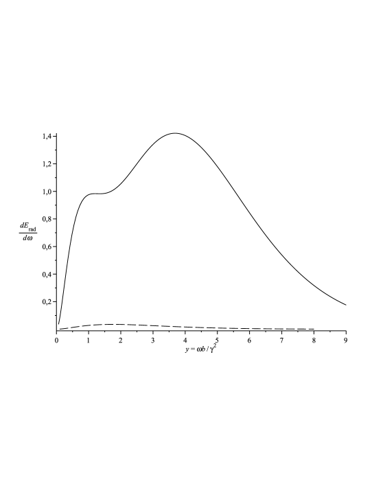
Figure 1: The contribution to the frequency distribution of the emitted energy of the real (solid line) and the imaginary (dashed line) part of $\rho$ for $D=6$ and $\gamma=20$. The two curves are rescaled by the same factor.

(d) $\rho^{\prime}(k)$ is also negligible. Using (VI.8) and (VI.21) one may convince oneself that in the lab frame the contribution to the total radiation (a) of the particle $m^{\prime}$ and (b) of the cross-term in (II.16) are both negligible in the ultra-relativistic limit. In particular, Figure 2 shows separately the contributions of $m$ (solid line) and $m^{\prime}$ (dashed line) to the emitted energy in the lab frame. So, the radiation from $m^{\prime}$ is important at very low frequencies, but may be neglected everywhere else, as well as in the total energy loss.

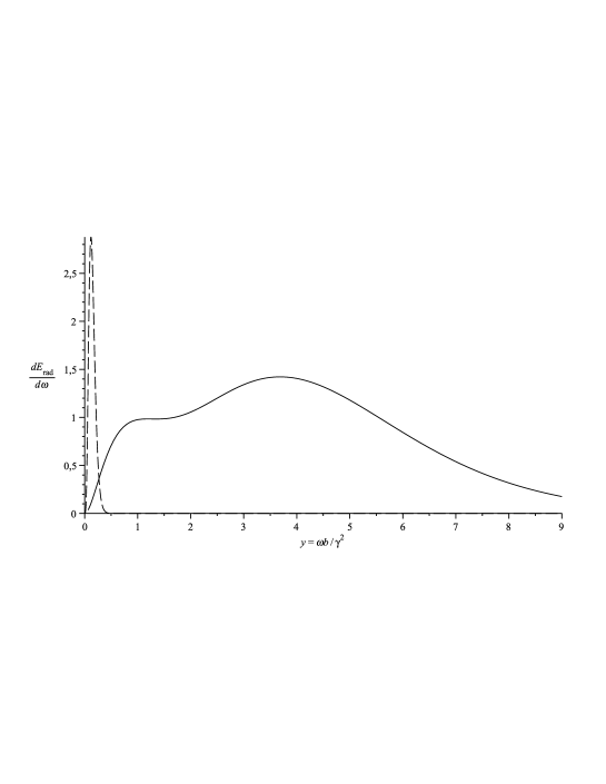
Figure 2: The relative contribution to the frequency distribution of the emitted energy of $\rho(k)$ (solid line) and $\rho^{\prime}(k)$ (dashed line) for $D=6$ and $\gamma=20$. The two curves are rescaled by the same factor.

Thus, we shall neglect the contribution of everything else but the real part of $\rho(k)$. This gives most of the energy lost in the collision.

(e) Finally, it is convenient to introduce the angle $\hat{\theta}$ by

$$\cos{\hat{\theta}}\equiv v,\quad\sin\hat{\theta}=1/\gamma.$$ (II.40)

Within the cone $0\leqslant\theta\leqslant\hat{\theta}$ the quantity $\xi$ for ultrarelativistic velocities remains small varying in the region $1/(2\gamma^{2})\leqslant\xi\leqslant 1/\gamma^{2}$. Note that for $\theta=\hat{\theta}$ the $m$-rest-frame radiation angle is $\theta_{0}=\pi/2$.

(f) The angular distribution $dE_{\mathrm{rad}}/d\theta$. As argued above, the leading contribution to the total energy loss is due to the real part of the amplitude $\rho(k)$, i.e.

$$\rho(k)\simeq{\rm Re}\;\rho(k)\simeq-\frac{f^{2}f^{\prime}}{(2\pi)^{n+1}mv^{3}\gamma^{3}b^{2n}}\left(\frac{1}{1-v\cos\theta}-\gamma^{2}\right)\;\hat{K}_{n}(z)\,,$$ (II.41)

which does not depend on angles other than the main polar angle $\theta.$

Substitute (II.41) into (II.16) and use (VI.8) to integrate over the frequencies. The result is the angular distribution of radiated energy:

$$\frac{dE_{\mathrm{rad}}}{d\Omega}=\frac{\sqrt{\pi}\,\Gamma\left(\frac{3D-9}{2}\right)\Gamma\left(\frac{2D-5}{2}\right)\Gamma\left(\frac{D-1}{2}\right)}{8(2\pi)^{2D-3}\Gamma(D-2)}\frac{f^{4}f^{\prime 2}}{b^{3D-9}\gamma^{6}m^{2}}\,\xi^{-(D+1)}\,\left(1-\gamma^{2}\xi\right)^{2}\,.$$ (II.42)

Integration over $\psi$ gives to leading ultra-relativistic order the $\theta-$distribution

$$\frac{dE_{\rm rad}}{d\theta}\simeq\frac{2^{4-3D}\Gamma\left(\frac{3D-9}{2}\right)\Gamma\left(\frac{2D-5}{2}\right)}{\pi^{3(D/2-1)}\Gamma^{2}\left(\frac{D-2}{2}\right)}\frac{f^{4}f^{\prime 2}}{b^{3D-9}\gamma^{6}m^{2}}\,\xi^{-(D+1)}\,\left(1-\gamma^{2}\xi\right)^{2}\,\sin^{D-3}\theta\,.$$ (II.43)

In the special case $f=f^{\prime}$ and $m=m^{\prime}$ one obtains for the radiation efficiency $\varepsilon_{d}\equiv E_{\rm rad}/E$

$$\frac{d\varepsilon_{d}}{d\theta}\simeq\frac{\Gamma\left(\frac{3+3d}{2}\right)\Gamma\left(\frac{3+2d}{2}\right)}{2^{8+3d}\,\pi^{3+3d/2}\Gamma^{2}\left(1+d/2\right)}\,\gamma^{-7}\left(\frac{r_{d}}{b}\right)^{3(1+d)}\xi^{-5-d}\left(1-\gamma^{2}\xi\right)^{2}\,\sin^{1+d}\theta\,,$$ (II.44)

plotted for various dimensions, $\gamma=500$ and $r_{d}/b=0.3$ in Figure 3.

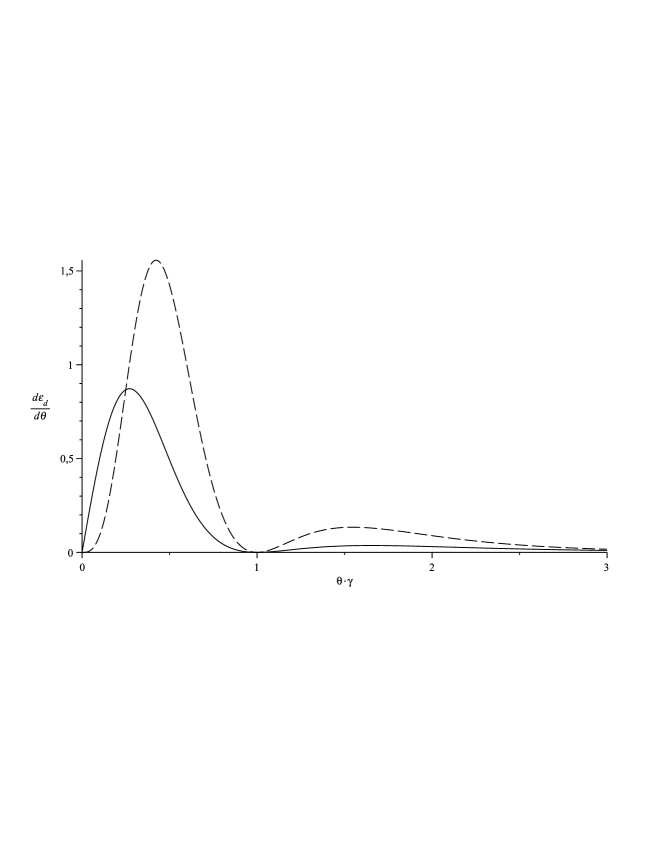
Figure 3: The angular distribution $d\varepsilon_{d}/d\theta$ versus $\theta/\hat{\theta}$ for $\gamma=500$, $r_{d}/b=0.3$ and for $d=0$ (solid line) and $d=2$ (dashed). The maxima are at $\theta_{1,2}\simeq\left[\frac{7+d\mp 2\sqrt{11+2d}}{5+d}\right]^{1/2}\hat{\theta}.$

(g) The frequency distribution $dE_{\rm rad}/d\omega$. Similarly, define $y\equiv\omega\,b/\gamma^{2}$ and substitute (II.41) into (II.16) to obtain

$$\frac{d\varepsilon_{d}}{dy}=\frac{\pi^{1+d/2}}{(2\pi)^{5+2d}\Gamma\left(\frac{2+d}{2}\right)}\gamma^{3+2d}\left(\frac{r_{d}}{b}\right)^{3(1+d)}y^{2+d}\!\!\int\!d\theta\left[1-(\gamma^{2}\xi)^{-1}\right]^{2}\hat{K}_{d/2}^{2}(y\gamma^{2}\xi)\sin^{1+d}\theta\,,$$ (II.45)

evaluated numerically and shown for various dimensions, $\gamma=500$ and $r_{d}/b=0.3$ in Figure 4.

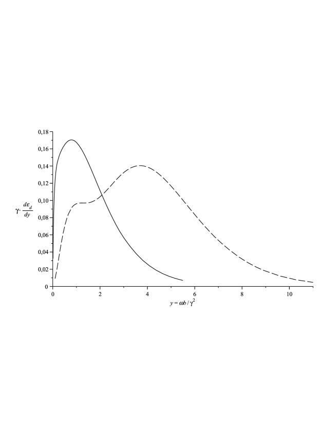
Figure 4: Frequency distribution $d\varepsilon_{d}/dy$ versus $y\equiv b\,\omega/\gamma^{2}$ for $\gamma=500$, $r_{d}/b=0.3$ and for $d=0$ (solid curve) and $d=2$ (dashed line).

II.2.4 The total radiated energy $E_{\mathrm{rad}}$

Finally, using (VI.5) one may integrate (II.43) over $\theta$ to obtain the leading ultra-relativistic limit of the radiation efficiency (for $m=m^{\prime}$ and $f=f^{\prime}$)

$$\varepsilon_{d}\equiv\frac{E_{\mathrm{rad}}}{E}\simeq{\mathcal{C}}_{d}\left(\gamma\,\frac{r_{d}^{3}}{b^{3}}\right)^{1+d},$$ (II.46)

with

$${\mathcal{C}}_{d}\equiv\frac{(2+d)\,\Gamma\left(\frac{3+3d}{2}\right)\Gamma\left(\frac{3+2d}{2}\right)}{2^{7+2d}\pi^{3(2+d)/2}\Gamma(4+d)}.$$ (II.47)

The radiation loss grows with $d$ as $\gamma^{2+d}$. For $d=0$

$$\varepsilon_{0}\simeq\frac{1}{3\times 2^{9}\,\pi^{2}}\;\gamma\,\left(\frac{r_{0}}{b}\right)^{3}$$

in agreement (modulo polarizations) with the corresponding formula in classical electrodynamics LandauII .

II.2.5 The bremsstrahlung cross-section $\sigma_{D}$

The energy differential cross-section with dimension (length)^2+d, i.e. the fraction of energy $d(E_{\rm rad}/E)$ emitted per unit time and per unit incoming beam flux $J\equiv dN/dA_{2+d}dt$ is given by:

$$d\sigma_{d}=\Omega_{1+d}b^{1+d}db\,d(E_{\rm rad}/E)=\frac{\Omega_{1+d}}{2(2\pi)^{3+d}m\gamma}|\rho(k)|^{2}b^{1+d}db\,\omega^{2+d}d\omega\,d\Omega_{2+d}\,,$$

with the volume of the unit $(n-1)-$dimensional sphere being $\Omega_{n-1}\equiv 2\pi^{n/2}/\Gamma(n/2)$. Its integral over $b$ from $b_{\rm min}$ to infinity is the frequency and angular distribution of the emitted energy fraction per unit time and unit incoming beam flux, while its total integral is the fraction of initial energy emitted per unit time and unit flux. Using (II.46) this is

$$\sigma_{d}=\frac{\Omega_{1+d}}{m\gamma}\int\limits_{b_{\rm min}}^{\infty}dE_{\rm rad}\,b^{1+d}\,db\simeq{\mathcal{C}}_{d}\,\frac{\Omega_{1+d}}{1+2d}\,r_{d}^{2+d}\,\gamma^{1+d}\,\left(\frac{r_{d}}{b_{\rm min}}\right)^{1+2d}\,.$$ (II.48)

II.2.6 The average number $\langle N\rangle$ of emitted quanta

A useful, though not classical, quantity to estimate is the number of emitted quanta. Divide the right hand side of (II.16) by the quantum energy $\hbar\omega$ to obtain

$$\frac{d{\langle N\rangle}}{d\omega d\Omega}\sim\frac{1}{2(2\pi)^{3+d}}\frac{\omega^{1+d}}{\hbar}|\rho(k)|^{2}\Big{|}_{k^{M}=\omega(1,\mathbf{n})},$$

substitute (II.41) and integrate, as above, over frequencies and angles to obtain an estimate of the total number of emitted $\Phi-$quanta, not counting the ones from $m^{\prime}$ with very low $\omega\to 0$ (see Figure 2)

$${\langle N\rangle}\sim\frac{\Gamma\left(\frac{2+3d}{2}\right)\Gamma^{2}\!\left(1+d\right)\Gamma^{2}\!\!\left(\frac{2+d}{2}\right)}{(3+d)\,2^{5-d}\pi^{4+3d/2}\Gamma(2+2d)\Gamma(2+d)}\,\frac{m\,r_{d}}{\hbar}\,\gamma^{d}\,\left(\frac{r_{d}}{b}\right)^{2+3d}\,.$$ (II.49)

III Scalar ultra-relativistic bremsstrahlung in $\mathbf{{\mathcal{M}}_{4}\times{\mathcal{T}}^{\,\textit{d}}}$

III.1 The model - General formalism

The above analysis is easily extended to study bremsstrahlung in the context of a scalar multidimensional model with the extra dimensions compactified on a torus ${\mathcal{T}}^{d}$. The model of interest describes two particles on the brane with masses $m$ and $m^{\prime}$, respectively, and two scalar fields. One, the ”scalar graviton” $\Phi$, lives in the $D=4+d$ dimensional bulk and is supposed to imitate gravity, while the other, $\phi$, lives on the 3-brane and mimics the Standard Model forces. The action of the model is

$$S_{\rm sc}=\frac{1}{2}\int d^{4}x\partial_{\mu}\phi\,\partial^{\mu}\phi\,+\frac{1}{2}\int d^{D}x\partial_{M}\Phi\,\partial^{M}\Phi-\sum_{\rm particles}\int d\tau\sqrt{\dot{z}^{2}}\left[m+e\phi(z)+f\Phi(z)\right]$$ (III.1)

with $\mu=0,1,2,3;\;M=0,1,\ldots,D-1$. $z^{\mu}(\tau)$ and $z^{\prime\mu}(\tau^{\prime})$ are the trajectories of the particles with masses $m$ and $m^{\prime}$, respectively. Notice that no $\Phi-\phi$ interaction is included, because it is not relevant in the leading order computation that follows. The coupling constants $e,e^{\prime}$ are dimensionless, while $f,f^{\prime}$ have length dimension $d/2$. With all radii of the torus taken for simplicity equal and denoted by $L$, the kinetic term of the zero mode of $\Phi$ is $(L^{d}/2)\int d^{4}x\partial_{\mu}\Phi\partial^{\mu}\Phi$. It is brought to the standard normalization by the rescaling $\Phi\to L^{-d/2}\Phi$, which converts the interaction term to $f_{4}\int d\tau\sqrt{\dot{z}^{2}}\Phi$ with the 4-dimensional coupling $f_{4}$ being

$$f_{4}=fL^{-d/2}\,.$$ (III.2)

The particles, apart from the radius $r_{d}$ defined in (II.2), are also characterized by the ”electromagnetic” classical radius, defined by

$$R_{0}\equiv e^{2}/m\,,$$ (III.3)

and similarly for the particle $m^{\prime}$ .

This simplified model is rich enough to study all four cases presented in Table 1, namely, the energy emitted in the bulk or on the brane, when the scattering of the two particles is dominated by either the $\Phi$ or the $\phi$ interactions. The cases of $\phi-$interaction with $\phi-$radiation on the brane and $\Phi-$ interaction with $\Phi-$radiation in the bulk are special cases of the previous section. The formalism necessary for the study of the crossed situations i.e. interaction via $\Phi(\phi)$ and $\phi(\Phi)-$radiation in the bulk, is the topic discussed next.

Retarded propagator for massive modes and particle trajectories. Denote the space-time coordinates by $x^{M}=\{x^{\mu},y^{i}\}$, with $\mu=0,1,2,3;\;i=1,\ldots,d$ and use bold letters to denote the $d-$vectors or the extra components of the $D-$vectors.

The retarded Green’s function of the d’Alembert equation

$$\Box_{D}G_{D}(x,x^{\prime},\mathbf{y}-\mathbf{y}^{\prime})=\delta^{4}(x-x^{\prime})\delta^{d}(\mathbf{y}-\mathbf{y}^{\prime})$$ (III.4)

is now expanded in Fourier series:

$$G_{D}(x-x^{\prime},\mathbf{y}-\mathbf{y}^{\prime})=\frac{1}{(2\pi)^{4}V_{d}}\int d^{4}p\,{\rm e}^{-ip\cdot(x-x^{\prime})}\sum_{\mathbf{n}\in{\mathbb{Z}}^{d}}\frac{{\rm e}^{i\bar{\bf n}\cdot(\mathbf{y}-\mathbf{y}^{\prime})}}{p^{2}-\bar{\rm n}^{2}+i\epsilon p^{0}},$$ (III.5)

where $\bar{\bf n}\equiv 2\pi\mathbf{n}/L,\;\bar{\rm n}\equiv\sqrt{\bar{\bf n}^{2}}$, and $V_{d}=L^{d}$ is the volume of extra space. Correspondingly, the solution of

$$\Box_{D}\Phi(x,\mathbf{y})=\rho_{D}(x,\mathbf{y})$$ (III.6)

with the source localized on the brane

$$\rho_{D}(x,\mathbf{y})=\rho(x)\delta^{d}(\mathbf{y})$$ (III.7)

is

$$\Phi(x,\mathbf{y})=\frac{1}{(2\pi)^{4}V_{d}}\int d^{4}p\,e^{-ip\cdot(x-x^{\prime})}\sum_{\mathbf{n}\in\mathbb{Z}^{d}}\frac{{\rm e}^{i\bar{\bf n}\cdot\mathbf{y}}}{{p}^{2}-\bar{\rm n}^{2}+i\epsilon p^{0}}\;\rho(x^{\prime})\;d^{4}x^{\prime}.$$ (III.8)

Its restriction to the 3-brane can be rewritten using the four-dimensional propagator

$$\Phi(x)\equiv\Phi(x,\mathbf{y})\Big{|}_{\mathbf{y}=0}=\int G_{4}(x-x^{\prime})\rho(x^{\prime})d^{4}x^{\prime},\quad G_{4}(x-x^{\prime})=G_{D}(x-x^{\prime},\mathbf{y}-\mathbf{y}^{\prime})\left.\vphantom{\sqrt{f}}\right|_{\mathbf{y}=\mathbf{y}^{\prime}=0},$$ (III.9)

whose Fourier transform is

$$G_{4}(p)=\frac{1}{V_{d}}\sum_{\mathbf{n}\in\mathbb{Z}^{d}}\frac{1}{{p}^{2}-\bar{\rm n}^{2}+i\epsilon p^{0}}.$$ (III.10)

In the four-dimensional language the massive scalar KK modes act as independent massive fields universally interacting with scalar charges through the total field

$$\Phi(x)=\sum_{\mathbf{n}\in\mathbb{Z}^{d}}\Phi_{\mathbf{n}}(x).$$ (III.11)

Thus, keeping four-dimensional conventions for the Fourier-transform, we can present the fields generated by the particle $m$ to lowest order as

$$\Phi_{\mathbf{n}}(q)=-\frac{2\pi f}{V_{d}}e^{iq\cdot z(0)}\delta(q\cdot u)\frac{1}{q^{2}-\bar{\rm n}^{2}},$$ (III.12)

and similarly for $m^{\prime}$. Taking into account only mutual particle interactions one obtains the lowest order corrections to the particles’ trajectories:

$$\delta z^{\mu}(\tau)=-i\frac{ff^{\prime}}{m(2\pi)^{D-1}V_{d}}\sum_{{\bf n}\in\mathbb{Z}^{d}}\int d^{4}q\frac{1}{q^{2}-\bar{\rm n}^{2}}\frac{1}{(q\cdot u)^{2}}\,{\rm e}^{-iq\cdot b}(e^{-i(q\cdot u)\tau}-1+iq\cdot u\tau)\delta(q\cdot u^{\prime})\Pi^{\mu\nu}q_{\nu}.$$ (III.13)

It can be checked that the corresponding corrections in the transverse directions

$$\delta\mathbf{y}=-i\frac{ff^{\prime}}{m(2\pi)^{D-1}V_{d}}\sum_{\mathbf{n}\in\mathbb{Z}^{d}}\int d^{4}q\frac{\bar{\bf n}}{q^{2}-\bar{\rm n}^{2}}\frac{1}{(q\cdot u)^{2}}\,{\rm e}^{-iq\cdot b}e^{-i(q\cdot u)\tau}\delta(q\cdot u^{\prime})=0$$

by parity and, as expected, the particles do not leave the brane.

$\Phi-$radiation flux. Consider a $(D-1)$-dimensional space-like hypersurface in the $D-$dimensional space-time and choose it for simplicity to be orthogonal to the time axis. The total $D-$momentum of the field $\Phi(x,\mathbf{y})$ associated with it reads:

$$P^{M}=\int_{\mathbb{R}^{3}\times T^{d}}T^{M0}d^{3}xd\mathbf{y}.$$ (III.14)

The field generated by a source localized on the brane is

$$\Phi(x,\mathbf{y})=\frac{1}{(2\pi)^{4}V_{d}}\int d^{4}k\sum_{\mathbf{n}\in\mathbb{Z}^{d}}\frac{\rho(k){\rm e}^{-ik\cdot x+i\bar{\bf n}\cdot\mathbf{y}}}{k^{2}-\bar{\rm n}^{2}+i\epsilon k^{0}},$$ (III.15)

where $\rho(k)$ is the four-dimensional Fourier-transform of the source. Substituting this into (III.14) and integrating over the three space and the torus, one obtains for $M=i$:

$$\mathbf{P}(t)\sim\int dk^{0}dk^{\prime 0}\sum_{\mathbf{n}\in\mathbb{Z}^{d}}\frac{\rho(k^{0},\underline{\bf k})\rho^{*}(k^{\prime 0},\underline{{\bf k}}){\rm e}^{i(k^{0}-k^{\prime 0})t}k^{0}\bar{\bf n}}{[(k^{0})^{2}-\underline{{\bf k}}^{2}-\bar{\rm n}^{2}][(k^{\prime 0})^{2}-\underline{{\bf k}}^{2}-\bar{\rm n}^{2}]},$$ (III.16)

where $\underline{{\bf k}}$ is a wave 3-vector on the brane. The sum vanishes by parity and reflects the expected fact that the radiation is emitted in the bulk symmetrically with respect to the brane.

Similarly, the change of the tangential to the brane components of the momentum of $\Phi$ between two space-like hypersurfaces $\Sigma_{\pm\infty}$ of topology $\mathbb{R}^{3}\times{\mathcal{T}}^{d}$ is again given by (II.12), or equivalently

$$P^{\mu}=\int d^{4}x\int_{V_{d}}d\mathbf{y}\nabla_{N}T^{\mu N},$$ (III.17)

from which

$$P^{\mu}=\int d^{4}x\int_{V_{d}}d\mathbf{y}\;(\rho_{D}+\rho_{D}^{\prime})\;\partial^{\mu}\Phi\,,$$ (III.18)

with the sources localized on the brane. Thus, the integral reduces to a four-dimensional one, and the retarded scalar field can be computed using the four-dimensional Green’s function. In particular, the energy emitted is

$$P^{0}\equiv E_{\rm rad}=\frac{1}{16\pi^{3}V_{d}}\sum_{\mathbf{n}\in\mathbb{Z}^{d}}\int\limits_{0}^{\infty}\!\!\omega^{2}d\omega\int\limits_{S^{2}}\!\!d\Omega\left.\vphantom{\sqrt{d}}|\rho^{\mathrm{tot}}(k)|^{2}\right|_{k^{0}=\sqrt{\omega^{2}+\bar{\rm n}^{2}}},$$ (III.19)

where $\omega=|\underline{\mathbf{k}}|$ and $\rho^{\mathrm{tot}}(k)$ is the four-dimensional Fourier-transform of the source.

III.2 Particles interact via $\Phi$ and emit $\phi-$radiation on the brane

Consider first the case in which the colliding particles interact mainly via $\Phi$. Technically one may take $e^{\prime}=0$ in (III.1). To compute the $\phi-$radiation emitted on the brane by particle $m$, one has to solve the field equation for $\phi$ with the source term of order $ff^{\prime}$. The radiation amplitude is the Fourier-transform of the source $\rho(k)$ on the mass-shell $k^{2}=0$ of $\phi$, while the radiation energy loss will be given by the $\bf n=0$ term in (III.19), or equivalently, by (II.16) with $D=4$ and $\rho^{\prime}=0$.

III.2.1 The emitted energy

The source $\rho(k)$ is of the form (II.23), with an obvious change in the couplings in front and summed over all KK modes. Using (V.18,V.19) relevant to the contribution of the generic massive mode $\bf n$, one obtains

$$\rho(k)=\frac{eff^{\prime}}{2\pi mL^{d}\gamma^{3}v^{4}z^{2}}\sum_{\mathbf{n}\in\mathbb{Z}^{d}}\left(bzK_{0}(Z_{\bar{\rm n}})(\gamma k\cdot u-k\cdot u^{\prime})+iv\hat{K}_{1}(Z_{\bar{\rm n}})k\cdot b\right),$$ (III.20)

with $Z_{\bar{\rm n}}\equiv\sqrt{z^{2}+\bar{\rm n}^{2}b^{2}}$.

The sum over the massive modes depends on the ratio $b/L$. For small $b/L$ a large number of modes will be excited and for a summand that depends only on the magnitude of $\bar{\rm n}$ one can write (see Appendix III for an estimate of the error due to this approximation)

$$\sum_{\mathbf{n}}f_{\mathbf{n}}\approx\int f_{\mathbf{n}}d\mathbf{n}=\frac{V_{d}}{(2\pi)^{d}}\Omega_{d-1}\int f_{\bar{\rm n}}\bar{\rm n}^{d-1}d\bar{\rm n}.$$ (III.21)

Define the new variable $w\equiv 1+(\bar{\rm n}b/z)^{2}$ and use formula GR (for $a,\mu>0$)

$$\int\limits_{1}^{\infty}\check{K}_{\nu}(a\sqrt{w})(w-1)^{\mu-1}dw=2^{\mu}a^{-2\mu}\Gamma(\mu)\check{K}_{\nu-\mu}(a)$$ (III.22)

to obtain

$$\sum_{\mathbf{n}\in\mathbb{Z}}\hat{K}_{\nu}(Z_{\bar{\rm n}})\approx\frac{(L/b)^{d}}{(2\pi)^{d/2}}\hat{K}_{\nu+d/2}(z),\qquad\nu\geqslant 0,$$ (III.23)

where $\check{K}_{\nu}(y)\equiv\hat{K}_{-\nu}(y)$. The resulting expression for the source coincides with the $(4+d)$-dimensional (II.30). According to the reasoning of Section II, the leading contribution to the emitted energy in the ultrarelativistic case comes from the first term inside the parenthesis of (III.20) and gives

$$\rho^{\mathrm{tot}}(k)\simeq\frac{eff^{\prime}}{(2\pi)^{d/2+1}\,mv^{3}\gamma^{3}b^{d}}(\gamma^{2}-\xi^{-1})\hat{K}_{d/2}(z).$$ (III.24)

Thus, with an appropriate correspondence of the couplings, the source looks the same as for the massless field in the case of non-compactified space-time of dimension $D=4+d$. The total emitted energy, however, will be different because of the different phase space in the two cases.

Substitution of (III.24) into (III.19) and integration over the frequencies leads to the angular distribution

$$\frac{dE_{\rm rad}}{d\Omega}=\frac{\Gamma\left(\frac{3+d}{2}\right)\Gamma\left(\frac{3+2d}{2}\right)}{2^{5}(2\pi)^{4+d}\,\Gamma\left(\frac{4+d}{2}\right)}\frac{e^{2}f^{2}f^{\prime 2}}{m^{2}\gamma^{6}b^{3+2d}}\,\xi^{-5}\,(1-\gamma^{2}\xi)^{2},$$

or equivalently (for $f=f^{\prime}$ and $m=m^{\prime}$)

$$\frac{d\varepsilon_{\Phi\phi}}{d\Omega}=\frac{\Gamma\left(\frac{3+d}{2}\right)\Gamma\left(\frac{3+2d}{2}\right)}{2^{5}(2\pi)^{4+d}\,\Gamma\left(\frac{4+d}{2}\right)}\frac{R_{0}}{b}\,\left(\frac{r_{d}}{b}\right)^{2+2d}\,\gamma^{-7}\,\xi^{-5}\,(1-\gamma^{2}\xi)^{2}.$$ (III.25)

Thus, up to the overall coefficient the angular distribution is the same as in $4D$ shown in Figure 3. No sign of extra dimensions in the angular profile of the radiation emitted on the brane, in contrast to the frequency distribution shown in Figure 5.

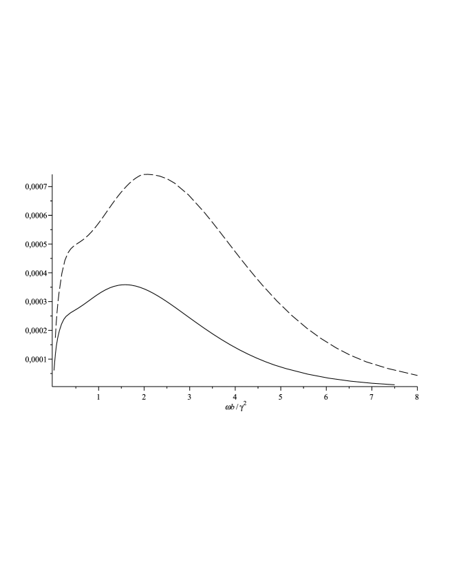
Figure 5: Frequency distribution $d\varepsilon_{d}/dy$ (d=1, solid curve) and $\gamma d\varepsilon/dy$ (d=2, dashed) versus $y\equiv b\,\omega/\gamma^{2}$, both for $\gamma=500$, $r_{d}/b=R_{0}/b=0.3$.

Finally, use

$$\int\limits_{0}^{2\pi}d\varphi\int\limits_{0}^{\pi}\sin\theta\,\xi^{-5}\,(1-\gamma^{2}\xi)^{2}\,d\theta=\frac{4\pi}{3}\gamma^{8}+\mathcal{O}(\gamma^{6}),$$

to integrate over the angles and obtain for the efficiency in the ultra-relativistic limit:

$$\varepsilon_{\Phi\phi}\simeq{\mathcal{C}}_{\Phi\phi}\,\frac{R_{0}}{b}\left(\frac{r_{d}}{b}\right)^{2(1+d)}\gamma\,,$$ (III.26)

with

$${\mathcal{C}}_{\Phi\phi}\equiv\frac{\Gamma\left(\frac{3+d}{2}\right)\Gamma\left(\frac{3+2d}{2}\right)}{3\cdot 2^{4}(2\pi)^{3+d}\,\Gamma\left(\frac{4+d}{2}\right)}\,.$$ (III.27)

As a check, notice that for $d=0$ and the identification $e=f$ it coincides with (II.46).

III.2.2 The cross-section $\sigma_{\Phi\phi}$

For the scattering process, which takes place on the 3-brane, the total cross-section for ultra-relativistic scattering is the integral of the differential energy cross-section

$$d\sigma_{\Phi\phi}=2\pi b\,db\,d\,\!E_{\rm rad}/m\gamma,$$ (III.28)

with $dE_{\rm rad}(\omega,\Omega,b)$ given above. Integration over the energy $\omega$ of the emitted scalar and the angles $\Omega=(\theta,\varphi)$ on the brane leads to $E_{\rm rad}(b)$ and upon integration over $b$ to (for $f=f^{\prime}$ and $m=m^{\prime}$)

$$\sigma_{\Phi\phi}\simeq\frac{2\pi}{1+2d}\,{\mathcal{C}}_{\Phi\phi}\,r_{d}^{2}\,\frac{R_{0}}{b_{\rm min}}\left(\frac{r_{d}}{b_{\rm min}}\right)^{2d}\,\gamma\,.$$ (III.29)

For $d=0$ it coincides with the corresponding expression derived in Section II.

III.3 Interaction via $\phi$ on the brane, emission of $\Phi$ in the bulk

Consider the action (III.1) with $f^{\prime}=0$. Now the particles interact only via the brane field $\phi$, but radiate both on the brane ($\phi$ and massless mode of $\Phi$) and in the bulk (massive modes $\mathbf{N}$ of $\Phi$). One wishes to estimate the amount of radiation into the bulk.

III.3.1 The energy radiated in the bulk

Following steps analogous to the ones above, one starts with the source for the $N-$th mode (eqn. (II.30) with $D=4$)

$$\rho^{(\mathbf{N})}(k)=-\frac{ee^{\prime}f}{2\pi\,L^{d}\,m\gamma^{3}\,v^{3}}\left[\left(\frac{\gamma z^{\prime}}{z}-\gamma^{2}\right){K}_{0}(z)+iv\sin\theta\sin\psi\hat{K}_{1}(z)/z\right],$$ (III.30)

with the arguments of the Macdonald functions in $\rho(k)$ and $\rho^{\prime}(k)$ being

$$z\equiv\frac{k\cdot ub}{\gamma v}=\frac{b}{v}\left(\sqrt{\omega^{2}+{\bar{N}}^{2}}-\omega v\cos\theta\right)\qquad{\rm and}\qquad z^{\prime}\equiv\frac{k\cdot u^{\prime}b}{\gamma v}=\frac{b}{\gamma v}\sqrt{\omega^{2}+{\bar{N}}^{2}}\,,$$ (III.31)

depending on the mode vector $\mathbf{N}.$

Next, one has to substitute (III.30) into (III.19), integrate over frequencies and angles and, finally, sum over the KK tower.

As in the previous cases, the main contribution to the emitted energy is due to the real part of the fast particle’s source. To compute it, introduce $\Xi\equiv k\cdot u/(\gamma k\cdot u^{\prime})$ and write

$$E_{\rm rad}=\frac{e^{2}e^{\prime 2}f^{2}\Omega_{d-1}}{2(2\pi)^{4+d}m^{2}\gamma^{6}}\sum_{\mathbf{N}\in\mathbb{Z}^{d}}\int_{0}^{\pi}\sin\theta\,d\theta\left(\Xi^{-1}-\gamma^{2}\right)^{2}\int_{0}^{\infty}\omega^{2}d\omega K_{0}^{2}(z).$$ (III.32)

Isolate the contribution of the massless mode and use (III.21) to convert to integration over masses. Then change to polar coordinates $(w,\alpha)$ by $\omega=w\cos\alpha,\;\bar{N}=w\sin\alpha$ with $0<\alpha<\pi/2$ and defining $\Xi=1-v\cos\alpha\cos\theta,$ integrate over $w$:

$$\int_{0}^{\infty}dww^{d+2}\,K_{0}^{2}(wb\Xi/v)=\frac{(v/b\Xi)^{d+3}2^{d}}{\Gamma(d+3)}\Gamma^{4}\left(\frac{d+3}{2}\right).$$

Then the leading in $\gamma$ contribution to the total emission in the bulk is given by

$$E_{\rm rad}=F\int\limits_{0}^{\pi/2}\cos^{2}\alpha\,\sin^{d-1}\alpha d\alpha\int\limits_{0}^{\pi}\frac{d\theta\sin\theta}{\Xi^{d+5}}\left(1-\gamma^{2}\Xi\right)^{2}\;,\;\;{\rm with}\;\;F\equiv\left(\frac{ee^{\prime}f}{m\gamma^{3}}\right)^{2}\frac{\Omega_{d-1}\,2^{d-1}\,\Gamma^{4}\left(\frac{d+3}{2}\right)}{(2\pi)^{4+d}\,\Gamma(d+3)\,b^{d+3}}.$$ (III.33)

The integral over $\theta$ can be converted into an integral over $\Xi$ from $\xi_{\alpha}\equiv 1-v\cos\alpha$ to $\bar{\xi}_{\alpha}\equiv 1+v\cos\alpha.$ The range of integration over $\alpha$ is such that one can omit the terms with $\bar{\xi}_{\alpha}$, and write

$$E_{\rm rad}\simeq F\int\limits_{0}^{\pi/2}\cos\alpha\sin^{d-1}\alpha\,d\alpha\left(\frac{\xi_{\alpha}^{-(d+4)}}{d+4}-2\gamma^{2}\frac{\xi_{\alpha}^{-(d+3)}}{d+3}+\gamma^{4}\frac{\xi_{\alpha}^{-(d+2)}}{d+2}\right),$$ (III.34)

with all remaining integrals of the form $V_{m}^{n}$ (VI.5) of the first kind ($2m>n+1$). The difference in the range of integration is insignificant, because it leads to ${\mathcal{O}}(\gamma^{-2})$ contribution in the integrals, which is negligible in the ultra-relativistic limit. Change the range of $\alpha$ integration to $[0,\pi]$ and use (VI.5) to evaluate (III.34). To leading order in $\gamma$ the result is (for $e=e^{\prime}$ and $m=m^{\prime}$)

$$\varepsilon_{\phi\Phi}\simeq{\mathcal{C}}_{\phi\Phi}\,(ee^{\prime}f_{4})^{2}\left(\frac{L}{b}\right)^{d}\frac{\gamma^{d+1}}{m^{3}\,b^{3}}\simeq{\mathcal{C}}_{\phi\Phi}\,\frac{R_{0}^{2}}{b^{2}}\,\left(\frac{r_{d}}{b}\right)^{d+1}\,\gamma^{d+1},$$ (III.35)

with

$${\mathcal{C}}_{\phi\Phi}=\frac{\Gamma^{3}\left(\frac{d+3}{2}\right)}{2^{5}\,\pi^{(d+7)/2}\,\Gamma(d+4)}.$$ (III.36)

III.3.2 The cross-section $\sigma_{\phi\Phi}$

Upon multiplication of (III.35) by $2\pi b\,db$ and integration over $b$ one obtains the total cross section

$$\sigma_{\phi\Phi}\simeq\frac{2\pi}{1+d}\,{\mathcal{C}}_{\phi\Phi}\,r_{d}^{2}\,\frac{R_{0}^{2}}{b_{\rm min}^{2}}\left(\frac{r_{d}}{b_{\rm min}}\right)^{-1+d}\gamma^{1+d}\,.$$

III.4 Interaction via $\Phi$ and $\Phi-$radiation in the bulk.

Consider, finally, the case in which the particles interact via exchange of $\Phi$ and emit $\Phi-$radiation in the bulk. Their couplings to $\Phi$ are $f$ and $f^{\prime}$, respectively. The source of radiation of the ${\bf N}-$th mode is then:

$$\rho^{(\mathbf{N})}(k)=-\frac{f^{2}f^{\prime}}{2\pi m\gamma^{3}v^{3}L^{d}}\sum_{\mathbf{n}}\left(\left(\frac{\gamma z^{\prime}}{z}-\gamma^{2}\right){K}_{0}(Z_{\bar{\rm n}})+iv^{2}\frac{\omega\sin\theta\sin\psi}{\sqrt{\omega^{2}+{\bar{N}}^{2}}z}\hat{K}_{1}(Z_{\bar{\rm n}})\right),$$ (III.37)

with the argument of the Macdonald functions being

$$Z_{\bar{\rm n}}=b\left[\left(\sqrt{\omega^{2}+{\bar{N}}^{2}}-\omega v\cos\theta\right)^{2}\!\!\!\left.\vphantom{\sqrt{f}}\right/v^{2}+\bar{\rm n}^{2}\right]^{1/2}$$ (III.38)

and the dimensionless products $k\cdot ub/\gamma v$ and $k\cdot u^{\prime}b/\gamma v$ given by (III.31).

Assuming again a large number of interaction modes, we replace the sum over modes by integration according to (III.21):

$$\rho^{(\mathbf{N})}(k)=-\frac{f^{2}f^{\prime}}{(2\pi)^{d/2+1}m\gamma^{3}v^{3}b^{d}}\left(\left(\frac{\gamma z^{\prime}}{z}-\gamma^{2}\right)\hat{K}_{d/2}(z)+iv^{2}\frac{\omega\sin\theta\sin\psi}{\sqrt{\omega^{2}+{\bar{N}}^{2}}z}\hat{K}_{1+d/2}(z)\right).$$ (III.39)

Thus, the argument of the Macdonald function corresponds to the massless interaction mode (III.30), so again the real part gives the main contribution to the emitted energy, which in polar coordinates ($w,\alpha$) in the $\omega-\bar{N}$ plane, becomes

$$\rho^{(\mathbf{N})}(k)=-\frac{f^{2}f^{\prime}}{(2\pi)^{d/2+1}m\gamma^{3}v^{3}b^{d}}\left(\Xi^{-1}-\gamma^{2}\right)\hat{K}_{d/2}(z),\quad\Xi\equiv 1-v\cos\alpha\cos\theta.$$ (III.40)

Substitute it in equation (III.19) and integrate over $w$, using:

$$\int_{0}^{\infty}dww^{d+2}\hat{K}_{d/2}^{2}(wb\Xi)=\frac{\sqrt{\pi}\Gamma\left(\frac{3d+3}{2}\right)\Gamma\left(\frac{2d+3}{2}\right)\Gamma\left(\frac{d+3}{2}\right)}{4\Gamma(d+2)(b\Xi)^{d+3}}.$$

Perform the remaining integrations over the angles $\varphi$, $\theta$ and $\alpha$ and use similar approximations to obtain for the leading ultra-relativistic contribution to the emitted energy ($f=f^{\prime}$, $m=m^{\prime}$)

$$\varepsilon_{\Phi\Phi}\simeq{\mathcal{C}}_{d}\,f_{4}^{4}{f^{\prime}}_{4}^{2}\left(\frac{L}{b}\right)^{3d}\frac{\gamma^{1+d}}{m^{3}\,b^{3}}\simeq{\mathcal{C}}_{d}\left(\frac{r_{d}}{b}\right)^{3+3d}\gamma^{1+d}\,,$$ (III.41)

with ${\mathcal{C}}_{d}$ given in (II.47). As expected, this expression is identical to the one obtained in the case of $D-$dimensional Minkowski space (II.46), even though the intermediate formulae and numerical coefficients in the phase space integrals are different, corresponding to different spatial topologies. This is a consequence of our approximation to convert mode summation to integration.

The corresponding energy cross-section is

$$\sigma_{\Phi\Phi}\simeq\frac{2\pi}{1+3d}\,{\mathcal{C}}_{d}\,f_{4}^{4}{f^{\prime}}_{4}^{2}\left(\frac{L}{b_{\rm min}}\right)^{3d}\frac{\gamma^{1+d}}{m^{3}\,b_{\rm min}}\simeq\frac{2\pi}{1+3d}\,{\mathcal{C}}_{d}\,r_{d}^{2}\left(\frac{r_{d}}{b_{\rm min}}\right)^{1+3d}\gamma^{1+d}\;.$$ (III.42)

IV Discussion - validity of the approximation - Prospects

An unambiguous classical computation of bremsstrahlung radiation in ultra-relativistic massive-particle collisions was presented in the context of a simplified scalar model in arbitrary dimensions, of which some may be compact. Scalar fields were used to model both the graviton in the bulk and the standard model interactions on the brane and the main results for the radiation efficiency are summarized in (I.1) and Table I. A quick glance at these leads to the following remarks: (a) In all cases there is enhancement of the efficiency by factors of $\gamma$. (b) Radiation emitted on the 3-brane is enhanced by one power of $\gamma$, while (c) each compact large extra dimension to which radiation can flow, contributes to the efficiency an extra power of $\gamma$.

A few comments are in order concerning the validity of our approximations. The leading order perturbative classical computation per se is a good approximation as long as the interaction energy is much smaller than the total available energy, i.e. $U(b)\sim f^{2}/b^{1+d}\ll E\simeq m\gamma$. On the other hand, the classical approach is relevant if one can justify (a) dealing with particle trajectories, and (b) treating radiation classically. As has been discussed in non-relativistic quantum mechanics landauIII and applied to the relativistic case as well giudice , requirement (a) implies (a1) small angle scattering and (a2) $|U^{\prime}(b)|\,b^{2}\gg\hbar$. Therefore, the impact parameter has to satisfy

$$\frac{r_{d}}{\gamma^{1/1+d}}\ll b\ll\left(\frac{f^{2}}{\hbar}\right)^{1/d}\equiv b_{c}\,.$$ (IV.1)

In addition, condition (b) of classicality of the radiation is written as

$$\langle N\rangle\sim\frac{m\,b}{\hbar\,\gamma}\,\left(\gamma\,\frac{r_{d}^{3}}{b^{3}}\right)^{1+d}\sim\frac{m\,b}{\hbar\,\gamma}\,\varepsilon_{d}\gg 1\,.$$ (IV.2)

Notice that for $\varepsilon_{d}\sim{\mathcal{O}}(1)$ the latter is satisfied for $m\,b\gg\hbar\,\gamma$, which is equivalent to $\hbar\,\omega_{\rm max}\sim\hbar\gamma^{2}/b\ll m\gamma$, which also has to be satisfied, since an emitted quantum cannot carry more than the total available energy. Finally, the deflection angle in the ultrarelativistic case is given for small momentum transfers $|t|\ll s$ by

$$\delta\alpha=\frac{|\dot{z}\cdot\Delta|}{|\Delta|\gamma}\Bigg{|}^{\tau\to\infty}_{\tau\to-\infty}=\lim_{\tau\to\infty}\frac{2iff^{\prime}}{m(2\pi)^{D-1}b\gamma}\int d^{D}q\frac{{\rm e}^{iq\cdot\Delta}\sin[(q\cdot u)\tau]\delta(q\cdot u^{\prime})(q\cdot\Delta)}{q^{2}(q\cdot u)},$$ (IV.3)

where $b\equiv|\mathbf{b}|$. Use $\displaystyle{\lim_{\tau\to\infty}\sin(q\cdot u\tau)/(q\cdot u)=\pi\delta(q\cdot u)}$ and perform the integration to obtain for $f=f^{\prime}$

$$\delta\alpha=\frac{1}{\Omega_{1+d}}\left(\frac{r_{d}}{b}\right)^{1+d}\frac{1}{\gamma^{2}}\,.$$ (IV.4)

The region of validity of this formula is $\delta\alpha\ll\sqrt{2/\gamma}\ll 1$ or equivalently $b\gg r_{d}\,\gamma^{-3/2(1+d)}$, and follows from the condition of small momentum transfer stated above.

For $\hbar\to 0$ the constraints are summarized to $b\gg r_{d}\,\gamma^{-1/1+d}$. Taking into account also the quantum constraints with $d\neq 0$ the impact parameter is restricted to $\hbar\gamma/m\ll b\ll b_{c}$, which requires (for $\hbar=1$) $\gamma\ll f_{4}^{2/d}mL$. In the special case of $d=0$ the region of validity of our approximation is $b\gg\hbar\gamma/m$.

The results of the present paper are suggestive, but by no means conclusive about gravitational bremsstrahlung itself. Gravity has many and significant differences from the toy scalar model. (a) In gravity there is an additional relevant scale $R_{g}=G_{N}\sqrt{s}$, which in principle enters the condition for the minimum classically reliable value of the impact parameter. (b) In addition, the fact that gravity couples to the energy-momentum is expected to lead to extra enhancement of radiation in the transplanckian regime. Finally, (c) gravity is non-linear with important effects due to these non-linearities. These qualitative features of classical transplanckian gravitational bremsstrahlung have been verified and presented briefly in gkst3 , while a longer detailed exposition is in preparation gkst4 .

V Appendix I: Momentum integrals

(a) Start with the following invariant integral

$$I\equiv mm^{\prime}\int d^{D}q\frac{\delta(q\cdot p^{\prime})\,\delta((k-q)\cdot p)\,{\rm e}^{-iq\cdot b}}{q^{2}}=\int d^{D}q\frac{\delta(q\cdot u^{\prime})\,\delta((k-q)\cdot u)\,{\rm e}^{-iq\cdot b}}{q^{2}}.$$ (V.1)

In the frame with $u^{\prime}=(1,0,...,0)$ one may immediately integrate over $dq^{0}\delta(q^{0})$ to obtain

$$I=-\int d^{D-1}\mathbf{q}\frac{\delta(k\cdot u+\mathbf{q\cdot u})\,{\rm e}^{i\mathbf{q\cdot b}}}{\mathbf{q}^{2}}.$$ (V.2)

Introduce $u^{\alpha}=\gamma(1,{\mathbf{v}})$, with $\gamma=1/{\sqrt{1-v^{2}}}$ and decompose $\mathbf{q}$ and $\mathbf{b}$ along $\mathbf{v}$ and perpendicular to it, writing $\mathbf{q}=q_{\|}\mathbf{n}+\mathbf{q}_{\bot}$, $\mathbf{b}=b_{\|}\mathbf{n}+\mathbf{b}_{\bot}$, where $\mathbf{n}=\mathbf{u}/\gamma v=\mathbf{v}/v$. It is straightforward to check that

$$b_{\|}=\frac{1}{\gamma v}\left(\gamma u^{\prime}\cdot b-u\cdot b\right)\;\;{\rm and}\;\;|\mathbf{b}_{\bot}|=\left(-b^{2}-\frac{[(u^{\prime}\cdot b)u-(u\cdot b)u^{\prime}]^{2}}{(u\cdot u^{\prime})^{2}v^{2}}\right)^{1/2}.$$ (V.3)

Integrating over $dq_{\|}$ with $\delta(k\cdot u+q_{\|}\gamma v)$ we obtain

$$I=-\frac{1}{\gamma v}{\rm e}^{-ik\cdot ub_{\|}/\gamma v}\int d^{D-2}\mathbf{q}_{\bot}\frac{{\rm e}^{i\mathbf{q_{\bot}\cdot b}_{\bot}}}{\mathbf{q}_{\bot}^{2}+(k\cdot u)^{2}/\gamma^{2}v^{2}}=-\frac{(2\pi)^{n+1}}{\gamma vb^{2n}}{\rm e}^{-ik\cdot ub_{\|}/\gamma v}\hat{K}_{n}(z),$$ (V.4)

where $n\equiv D/2-2$, $z\equiv k\cdot ub/\gamma v$, $\hat{K}_{\lambda}(w)\equiv w^{\lambda}K_{\lambda}(w)$ and $b\equiv|\mathbf{b_{\bot}}|$ now. For $b_{\|}\sim\mathbf{u}\cdot\mathbf{b}=0$ (the case of interest in the main text) the above simplifies to

$$I=-\frac{(2\pi)^{n+1}}{\gamma vb^{2n}}\;{\hat{K}}_{n}(z).$$ (V.5)

Correspondingly, the primed integral obtained by a $u\leftrightarrow u^{\prime}$ and $b_{M}\leftrightarrow-b_{M}$ exchange,

$$I^{\prime}\equiv\int d^{D}q\frac{\delta(q\cdot u)\delta((k-q)\cdot u^{\prime})\,{\rm e}^{iq\cdot b}}{q^{2}}=-\frac{(2\pi)^{n+1}}{\gamma vb^{2n}}\hat{K}_{n}(z^{\prime})$$ (V.6)

with $z^{\prime}\equiv k\cdot u^{\prime}b/\gamma v$.

(b) Consider next the vectorial integral

$$I_{M}\equiv\int d^{D}q\;\frac{\delta(q\cdot u^{\prime})\delta((k-q)\cdot u)\,{\rm e}^{-iq\cdot b}}{q^{2}}\;q_{M}.$$ (V.7)

It may be computed with the help of

$$I_{M}=i\frac{\partial I}{\partial b^{M}}=i\left(\frac{\partial I}{\partial b_{\|}}\frac{\partial b_{\|}}{\partial b^{M}}+\frac{\partial I}{\partial b}\frac{\partial b}{\partial b^{M}}\right)$$ (V.8)

Its explicit fully covariant form is obtained using (V.4) and (V.3)

$$\frac{\partial I}{\partial b_{\|}}=i\frac{k\cdot u}{\gamma v}I\;,\;\;\frac{\partial I}{\partial b}=-\frac{I}{b}\frac{\hat{K}_{n+1}(z)}{\hat{K}_{n}(z)},$$ (V.9)

where use was made of the formulae

$$K^{\prime}_{n}(z)=-K_{n-1}(z)-\frac{n}{z}K_{n}(z)=-K_{n+1}(z)+\frac{n}{z}K_{n}(z),$$

$$\hat{K}^{\prime}_{n}(z)=-z\hat{K}_{n-1}(z),\qquad\check{K}^{\prime}_{n}(z)=-z\check{K}_{n+1}(z).$$ (V.10)

Using

$$\frac{\partial b_{\|}}{\partial b^{M}}=-\frac{\gamma u^{\prime}_{M}-u_{M}}{\gamma v}\;,\;\;\frac{\partial b}{\partial b^{M}}=-\frac{1}{b}\left(b_{M}+\frac{(u^{\prime}\cdot b-u\cdot b\;\gamma)u^{\prime}_{M}+(u\cdot b-u^{\prime}\cdot b\;\gamma)u_{M}}{(u\cdot u^{\prime})^{2}v^{2}}\right),$$ (V.11)

one is led to the final result

$$I_{M}=-\frac{(2\pi)^{n+1}}{\gamma vb^{2n+2}}\left(\frac{bz}{\gamma v}(\gamma u^{\prime}_{M}-u_{M})\hat{K}_{n}(z)+ib_{M}\hat{K}_{n+1}(z)\right).$$ (V.12)

(c) The integral

$$I^{(A)}\equiv\int d^{D}q\frac{\delta(q\cdot u^{\prime})\delta((k-q)\cdot u)\,{\rm e}^{iq\cdot b}}{(q\cdot u)^{A}\;q^{2}}=\int d^{D}q\frac{\delta(qu^{\prime})\delta((k-q)u)\,{\rm e}^{iq\cdot b}}{(q_{0}u_{0}-q_{\|}\gamma v)^{A}\;q^{2}}$$ (V.13)

after integration over $dq^{0}\delta(q^{0})$ gives the extra factor $(-\mathbf{q\cdot u})^{-A}$, which by virtue of $d(\mathbf{q\cdot u})\delta(ku+\mathbf{q\cdot u})/\gamma v$ gives $1/(k\cdot u)^{A}$. Thus

$$I^{(A)}(k)=\frac{I}{(k\cdot u)^{A}}.$$ (V.14)

Similarly, for the vectorial integrals

$$I_{M}^{(A)}\equiv\int d^{D}q\frac{\delta(q\cdot u^{\prime})\delta((k-q)\cdot u)\,{\rm e}^{iq\cdot b}}{(q\cdot u)^{A}\;q^{2}}q_{M}=\frac{I_{M}}{(k\cdot u)^{A}},$$ (V.15)

Similar relations hold for the primed integrals. The denominators are $(k\cdot u^{\prime})^{A}$.

(d) In the case of ${\mathcal{M}}_{4}\times{\mathcal{T}}^{d}$ space-time, one is led to the invariant integral

$$I_{\bar{\rm n}}=\int d^{4}q\frac{\delta(q\cdot u^{\prime})\delta((k-q)\cdot u)\,{\rm e}^{iq\cdot b}}{q^{2}-\bar{\rm n}^{2}},$$ (V.16)

where $\bar{\rm n}=\sqrt{\bar{\bf n}^{2}}$ and $\bar{\bf n}=2\pi\mathbf{n}/L,\,\mathbf{n}\in\mathbb{Z}^{d}$. It is computed in the same way. After the $q^{0}$-integration, the denominator becomes $\mathbf{q}^{2}+\bar{\rm n}^{2}+(k\cdot u/\gamma v)^{2},$ and leads to

$$I_{\bar{\rm n}}=-\frac{2\pi}{\gamma v}{K}_{0}(Z_{\bar{\rm n}}),$$ (V.17)

with $Z_{\bar{\rm n}}\equiv\sqrt{z^{2}+\bar{\rm n}^{2}b^{2}}$ and $z=k\cdot u\;b/(\gamma v)$. If $\mathrm{m}$ represents the single one-dimensional KK mass $m_{l}$, we will refer to $Z_{l}\equiv\sqrt{z^{2}+m_{l}^{2}b^{2}}$ and to the integral $I_{l}$ respectively.

(e) The vectorial integral can be computed by differentiation and the result is

$$I^{M}_{\bar{\rm n}}\equiv\int d^{4}q\frac{\delta(q\cdot u^{\prime})\,\delta((k-q)\cdot u)\,{\rm e}^{iq\cdot b}}{q^{2}-\bar{\rm n}^{2}}\;q^{M}=-\frac{2\pi}{\gamma vb^{2}}\left(bz{K}_{0}(Z_{\bar{\rm n}})\frac{\gamma u^{\prime M}-u^{M}}{\gamma v}+i\hat{K}_{1}(Z_{\bar{\rm n}})b^{M}\right).$$ (V.18)

Analogously, if the integrals have the factor in the denominator $(q\cdot u)^{s}$ of the integrand, give the additional factor $(k\cdot u)^{-s}$ by virtue of the delta-function $\delta((k-q)\cdot u)$, namely one obtains

$$I^{(s)}_{\bar{\rm n}}=I_{\bar{\rm n}}\;(k\cdot u)^{-s}\qquad I^{(s)M}_{\bar{\rm n}}=I^{\prime M}_{\bar{\rm n}}\;(k\cdot u)^{-s}.$$ (V.19)

Analogous relations hold for the primed integrals.

VI Appendix II

VI.1 Angular integrals

(a) In the main text the following angular integrals $\theta$ were needed for integer $m$ and $n$

$$V_{m}^{n}\equiv\int\limits_{0}^{\pi}\frac{\sin^{n}\theta}{\xi^{m}}d\theta,\qquad\xi=1-v\cos{\theta}.$$ (VI.1)

Making use of the formula Proudn , valid for any real $a>|b|$, and $\mathrm{Re}\,{\nu}>0$:

$$\int\limits_{0}^{\pi}\frac{\sin^{2\nu-1}{\theta}}{(a+b\cos{\theta})^{\mu}}d\theta=\left(-\frac{2}{b}\right)^{\nu-1/2}\!\!\!\!\sqrt{\pi}\Gamma{(\nu)}(a^{2}-b^{2})^{(\nu-\mu)/2-1/4}P^{1/2-\nu}_{\nu-\mu-1/2}\left(\frac{a}{\sqrt{a^{2}-b^{2}}}\right),$$ (VI.2)

we express the result in terms of the associated Legendre function $P^{\mu}_{\nu}(z)$. In our case $a=1,b=-v,$ so:

$$V_{\mu}^{2\nu-1}=\left(\frac{2}{v}\right)^{\nu-1/2}\!\!\!\!\sqrt{\pi}\Gamma{(\nu)}\gamma^{-\nu+\mu+1/2}P^{1/2-\nu}_{\nu-\mu-1/2}\left(\gamma\right)=\left(\frac{2}{v}\right)^{n/2}\!\!\!\!\sqrt{\pi}\Gamma\left(\frac{n+1}{2}\right)\gamma^{-n/2+\mu}P^{-n/2}_{n/2-\mu}(\gamma).$$ (VI.3)

For $\gamma\gg 1,$ one can use the asymptotic formula GR :

$$P^{\lambda}_{\rho}(z)=\left(\frac{2^{\rho}\Gamma(\rho+1/2)}{\sqrt{\pi}\Gamma(\rho-\lambda+1)}z^{\rho}+\frac{\Gamma(-\rho-1/2)}{2^{\rho+1}\sqrt{\pi}\Gamma(-\rho-\lambda)}z^{-\rho-1}\right)(1+O(1/z^{2})).$$ (VI.4)

For $2m>n+1$ one finds to leading order

$$V_{m}^{n}= \frac{2^{m-1}}{v^{n/2}\Gamma(m)}\Gamma\left(\frac{n+1}{2}\right)\Gamma\left(m-\frac{n+1}{2}\right)\gamma^{2m-n-1},$$ (VI.5)

while for $2m<n+1$

$$V_{m}^{n}=\frac{2^{n-m}}{v^{n/2}}\frac{\Gamma\left(\frac{n+1}{2}\right)\Gamma\left(\frac{n+1}{2}-m\right)}{\Gamma(n-m+1)}.$$ (VI.6)

In the case $2m=n+1$ an expansion of the integral is logarithmic.

(b) Another integral used in the main text is:

$$\int_{S^{D-3}}|\sin\psi|^{N}d\Omega=\frac{2\pi^{(D-3)/2}\Gamma\left(\frac{{N+1}}{2}\right)}{\Gamma\left(\frac{D-2+N}{2}\right)}.$$ (VI.7)

VI.2 Integrals of products of Macdonald functions

Computation of integrals over the frequency or the impact parameter involving products of two Macdonald functions of the same argument is performed using the formula Proudn :

$$\int\limits_{0}^{\infty}K_{\mu}(cz)K_{\nu}(cz)z^{\alpha-1}dz=\frac{2^{\alpha-3}\Gamma\left(\frac{\alpha+\mu+\nu}{2}\right)\Gamma\left(\frac{\alpha+\mu-\nu}{2}\right)\Gamma\left(\frac{\alpha-\mu+\nu}{2}\right)\Gamma\left(\frac{\alpha-\mu-\nu}{2}\right)}{c^{\alpha}\Gamma(\alpha)}.$$ (VI.8)

Actually, only such integrals are needed in this work. More general integrals involving functions of different arguments arise from interference terms. They can be computed using the formula

$$K_{\nu}(\lambda z)=\lambda^{\nu}\sum_{k=0}^{\infty}\frac{1}{k!}\frac{z^{k}}{2^{k}}(1-\lambda^{2})^{k}K_{\nu+k}(z)\;,\qquad|1-\lambda^{2}|<1.$$ (VI.9)

The typical integral

$$\Theta=\int\limits_{0}^{\infty}K_{\nu}(z)K_{\nu^{\prime}}(z^{\prime})z^{m}z^{\prime m^{\prime}}\omega^{D-2}d\omega,$$ (VI.10)

where $z=z^{\prime}\gamma\xi$, can be cast for $\gamma\xi<1$ (i.e. $0\leqslant\theta\lesssim\sqrt{2/\gamma}$) into the form

$$(\gamma\xi)^{m}\left(\frac{\gamma v}{\rho}\right)^{D-1}\int\limits_{0}^{\infty}K_{\nu}(\gamma\xi z^{\prime})K_{\nu^{\prime}}(z^{\prime})z^{\prime m+m^{\prime}}z^{\prime D-2}dz^{\prime},$$ (VI.11)

and for $\gamma\xi>1$ ($\sqrt{2/\gamma}\lesssim\theta\leqslant\pi$) to

$$\frac{1}{(\gamma\xi)^{m^{\prime}}}\left(\frac{\gamma v}{\rho}\right)^{D-1}\int\limits_{0}^{\infty}K_{\nu}(z)K_{\nu^{\prime}}(z/\gamma\xi)z^{m+m^{\prime}}z^{D-2}dz.$$ (VI.12)

One is interested in an estimate of (VI.10) in powers of $\gamma\gg 1$. Use (VI.9) to write

$$\Theta\!=\!\left\{\begin{array}[]{ll}\displaystyle\!\!\!(\gamma\xi)^{m+\nu}\left(\frac{\gamma v}{\rho}\right)^{D-1}\sum_{k=0}^{\infty}\frac{1}{2^{k}k!}(1-\gamma^{2}\xi^{2})^{k}\int\limits_{0}^{\infty}z^{\prime k}K_{\nu+k}(z^{\prime})K_{\nu^{\prime}}(z^{\prime})z^{\prime m+m^{\prime}}z^{\prime D-2}dz^{\prime},&\hbox{$\gamma\xi<1$;}\\ \displaystyle\!\!\!\frac{1}{(\gamma\xi)^{m^{\prime}+\nu^{\prime}}}\left(\frac{v}{\xi\rho}\right)^{D-1}\sum_{k=0}^{\infty}\frac{1}{2^{k}k!}\left(1-\frac{1}{\gamma^{2}\xi^{2}}\right)^{k}\int\limits_{0}^{\infty}z^{k}K_{\nu}(z)K_{\nu^{\prime}+k}(z)z^{m+m^{\prime}}z^{D-2}dz\!\!,&\hbox{$\gamma\xi>1$.}\\ \end{array}\right.$$ (VI.15)

Denote by $M\equiv m+m^{\prime}+D-1$ and integrate over $z$ with the help of (VI.8). The integral in (VI.15,a) is equal to

$$\textstyle\frac{2^{M-3+k}}{\Gamma(M+k)}\Gamma\left(\frac{M+2k+\nu+\nu^{\prime}}{2}\right)\Gamma\left(\frac{M+2k+\nu-\nu^{\prime}}{2}\right)\Gamma\left(\frac{M+\nu^{\prime}-\nu}{2}\right)\Gamma\left(\frac{M-\nu^{\prime}-\nu}{2}\right),$$ (VI.16)

while the one in (VI.15,b) is related to the above by the exchange $\nu\leftrightarrow\nu^{\prime}$.

Given that for fixed $\lambda>0$ the function $\Gamma(x)\Gamma(\lambda-x)$ is decreasing for $x$ in $[0,\lambda/2]$ and increasing in $[\lambda/2,\lambda]$, one obtains the inequality

$$\textstyle\Gamma\left(\frac{M+2k+\nu+\nu^{\prime}}{2}\right)\Gamma\left(\frac{M+2k+\nu-\nu^{\prime}}{2}\right)<\Gamma(M+k)\Gamma(\nu+k),$$ (VI.17)

which leads to the estimate

$$\Theta<\left\{\begin{array}[]{ll}\!\!\!2^{M-3}\Gamma\left(\frac{M+\nu^{\prime}-\nu}{2}\right)\Gamma\left(\frac{M-\nu^{\prime}-\nu}{2}\right)(\gamma\xi)^{m+\nu}\left(\gamma v/\rho\right)^{\scriptscriptstyle D-1}\sum\limits_{\scriptscriptstyle k=0}^{\scriptscriptstyle\infty}(1-\gamma^{2}\xi^{2})^{k}\Gamma(\nu+k)/k!,&\hbox{$\gamma\xi<1$;}\\ \!\!\!2^{M-3}\Gamma\left(\frac{M+\nu-\nu^{\prime}}{2}\right)\Gamma\left(\frac{M-\nu^{\prime}-\nu}{2}\right)(\gamma\xi)^{-(m^{\prime}+\nu^{\prime})}\left(v/\xi\rho\right)^{\scriptscriptstyle D-1}\sum\limits_{\scriptscriptstyle k=0}^{\scriptscriptstyle\infty}\left(1-\frac{1}{\gamma^{2}\xi^{2}}\right)^{k}\!\!\Gamma(\nu^{\prime}+k)/k!,&\hbox{$\gamma\xi>1$.}\\ \end{array}\right.$$

Both series are summable because

$$\sum_{k=0}^{\infty}\frac{1}{k!}(1-a^{2})^{k}\Gamma(n+k)=\frac{\Gamma(n)}{a^{2n}},\qquad|a|<1,$$ (VI.18)

and give the following upper bounds, which are enough for our purposes:

$$\!\!\!\Theta\!<\!\left\{\begin{array}[]{ll}\!\!\!2^{M-3}\Gamma\!\left(\frac{M+\nu^{\prime}-\nu}{2}\right)\Gamma\!\left(\frac{M-\nu^{\prime}-\nu}{2}\right)\Gamma(\nu)\left(\frac{\gamma v}{\rho}\right)^{D-1}\!\!\!\!(\gamma\xi)^{m-\nu}\!\!,&\hbox{$\gamma\xi<1$;}\\ \!\!\!2^{M-3}\Gamma\!\left(\frac{M+\nu-\nu^{\prime}}{2}\right)\Gamma\!\left(\frac{M-\nu^{\prime}-\nu}{2}\right)\Gamma(\nu^{\prime})\left(\frac{v}{\xi\rho}\right)^{D-1}\!\!\!\!(\gamma\xi)^{\nu^{\prime}-m^{\prime}}\!\!,&\hbox{$\gamma\xi>1$.}\\ \end{array}\right.$$ (VI.21)

For $\nu=\nu^{\prime}$ the estimate is continuous at $\theta=\arccos((\gamma-1)/\gamma v).$

VII Appendix III

VII.1 Effective number of interacting $\Phi-$KK modes

In this subsection we would like to count the effective number of contributing interaction KK modes of the bulk field $\Phi$, studied in Subsection III.B, and estimate the error due to the replacement of the summation over those by integration.

Start with the case $D=5$, i.e. with one-dimensional mass sequence. It was argued that the dominant contribution to the energy loss comes from the first term in the parenthesis of (III.20) and requires the evaluation of the two-parameter integrals

$$G(\alpha,\beta)=\int\limits_{0}^{\infty}\!K_{0}\!\left(\!\!\sqrt{z^{2}+\alpha^{2}}\right)K_{0}\!\left(\!\!\sqrt{z^{2}+\beta^{2}}\right)z^{2}dz,$$ (VII.1)

for $\alpha\geqslant 0,\beta\geqslant 0$ and $\alpha+\beta>0$. Using the integral representation GR

$$K_{\nu}(x)K_{\nu}(y)=\frac{1}{2}\int\limits_{0}^{\infty}\exp\left[-\frac{t}{2}-\frac{x^{2}+y^{2}}{2t}\right]K_{\nu}\left(\frac{xy}{t}\right)\frac{dt}{t},$$ (VII.2)

we obtain the following approximation $\tilde{G}(\alpha,\beta)$ for $G$:

$$\tilde{G}(\alpha,\beta)\simeq\frac{\pi^{2}}{32}e^{-(\alpha+\beta)}\left(1+\frac{2^{7}\alpha^{2}\beta^{2}}{\pi(\alpha+\beta)^{3}}\right)^{1/2}.$$ (VII.3)

In view of the exponential fall-off of $\tilde{G}$ it is natural to separate the modes to light for $\alpha+\beta<2$ and heavy for $\alpha+\beta>2$. The choice $\alpha+\beta=2$ for the boundary is justified by just looking at the numerical plots. For the heavy modes one can neglect the unity in the parenthesis of (VII.3) and write

$$\tilde{G}(\alpha,\beta)\approx\frac{\sqrt{2}}{4}\pi^{3/2}e^{-(\alpha+\beta)}\frac{\alpha\beta}{(\alpha+\beta)^{3/2}}\;,\qquad\alpha+\beta>2$$ (VII.4)

Correspondingly, for the light modes one may take approximately

$$\tilde{G}(\alpha,\beta)\approx\frac{\pi^{2}}{32}e^{-(\alpha+\beta)},\qquad\alpha+\beta<2.$$ (VII.5)

In the cases of interest here $\alpha=2\pi b\,l/L,\beta=2\pi b\,l^{\prime}/L$ with integer $l$ and $l^{\prime}$. Thus, denoting by $K\equiv l+l^{\prime},$ one sees that the integer part

$$K_{c}=[L/(\pi b)]$$ (VII.6)

defines the boundary between light ($K<K_{c}$) and heavy ($K>K_{c}$) modes. If $L<\pi b$, there are no light modes in this classification. In the sequel only the case $L>\pi b$ ($K_{c}>1$) will be discussed.

To estimate separately the contributions of the light (heavy) interaction modes to the emitted energy, substitute the first term of (III.20) into (II.16) and integrate over angles, using (VII.5) and (VII.4), respectively. For the light modes one obtains (up to coefficients)

$$\sum G_{\rm light}\simeq\frac{\pi^{2}}{32}\sum_{K=1}^{K_{c}}e^{-2\pi Kb/L}(K+1),\qquad K_{c}\geqslant 1.$$ (VII.7)

It is easy to sum the geometric series for any $K_{c}$. In particular, for $K_{c}\gg 1$ the highest power in $K_{c}$ gives

$$\sum G_{\rm light}\simeq\frac{\Lambda_{\rm light}\pi^{2}}{32}K_{c}^{2},\qquad K_{c}\gg 1,$$ (VII.8)

with $\Lambda_{\rm light}\equiv 1/4-3/(4{\rm e}^{2})\thickapprox 0.148\thickapprox 1/7.$ Similarly, the heavy modes give

$$\sum G_{\rm heavy}\simeq\frac{\pi^{3/2}}{2K_{c}^{1/2}}e^{-(\alpha+\beta)}\!\!\!\!\sum_{K=K_{c}+1}^{\infty}\frac{e^{-2K/K_{c}}}{K^{3/2}}\sum_{l=0}^{K}l(K-l)\simeq\frac{\pi^{3/2}}{12K_{c}^{1/2}}\!\!\sum_{K=K_{c}+1}^{\infty}{\rm e}^{-2K/K_{c}}K^{3/2}.$$ (VII.9)

Replacing the sum over $K$ by integration from $K_{c}$ to $\infty$, one obtains for large $K_{c}$:

$$\sum G_{\rm heavy}\simeq\frac{\Lambda_{\rm heavy}\pi^{3/2}}{3\cdot 2^{9/2}}K_{c}^{2},\qquad K_{c}\gg 1,$$ (VII.10)

with $\Lambda_{\rm heavy}=7/(\sqrt{2}{\rm e}^{2})+3\sqrt{\pi}\left[1-\Phi\left(\sqrt{2}\right)\right]/4\approx 0.73\thickapprox 5/7$, where $\Phi$ is the Laplace’s error function. In the case $L<\pi b$ (no light modes) one should integrate from 0 to $\infty$ and substitute $K_{c}\to L/(\pi b)$ in (VII.10).

Using (VII.8) and (VII.10) one obtains the following ratio for $d=1$:

$$\frac{\Delta E_{\rm light}}{\Delta E_{\rm heavy}}\approx\frac{3\pi^{1/2}\Lambda_{\rm light}}{2^{1/2}\Lambda_{\rm heavy}}=0.76\approx 3/4.$$ (VII.11)

Thus, despite the fact that each heavy mode is exponentially suppressed their total contribution is comparable to the one of the light modes.

The above generalizes to arbitrary $d>1$. One has to integrate over the domain $W$ defined as $M\equiv\bar{\rm n}+\bar{\rm n}^{\prime}<2\pi K_{c}/L\equiv M_{c}$ which represents the multidimensional bispherical octahedron (the coefficient $\pi^{2}/32$ is omitted):

$$\sum G^{(d)}_{\rm light}\simeq\frac{(V_{d}\Omega_{d-1})^{2}}{(2\pi)^{2d}}\int\limits_{W}{\rm e}^{-2M/M_{c}}(\bar{\rm n}\,\bar{\rm n}^{\prime})^{d-1}d\bar{\rm n}\,d\bar{\rm n}^{\prime}\simeq\frac{\Omega_{d-1}^{2}}{2^{2d}}\mathrm{B}(d,d)\gamma(2d,2)\,K_{c}^{2d},$$ (VII.12)

with $\gamma(x,y)$ is the lower incomplete gamma-function, $\mathrm{B}(x,y)$ is the Euler beta-function. The corresponding heavy mode contribution reads:

$$\sum G^{(d)}_{\rm heavy}\simeq\frac{2^{7/2}(V_{d}\Omega_{d-1})^{2}}{\pi^{1/2}(2\pi)^{2d}}\int\limits_{\overline{W}}\frac{{\rm e}^{-2M/M_{c}}}{M^{3/2}}(\bar{\rm n}\,\bar{\rm n}^{\prime})^{d}d\bar{\rm n}\,d\bar{\rm n}^{\prime}\simeq\frac{\Omega_{d-1}^{2}\,\mathrm{B}(d+1,d+1)\,\Gamma(2d+1/2,2)}{2^{2d-7/2}\pi^{1/2}}\,K_{c}^{2d}\,,$$ (VII.13)

with $\Gamma(x,y)$ the upper incomplete gamma-function. Thus, the ratio is

$$\frac{\sum G^{(d)}_{\rm light}}{\sum G^{(d)}_{\rm heavy}}\simeq\frac{\pi^{1/2}\mathrm{B}(d,d)\gamma(2d,2)}{2^{7/2}\mathrm{B}(d+1,d+1)\Gamma(2d+1/2,2)}\,,$$ (VII.14)

a decreasing function of $d$.

Add (VII.12) with (VII.13) for the emitted energy in $D-$dimensions and compare to the energy loss $\Delta E_{4}$ in the purely four-dimensional case to obtain the estimate

$$\frac{\Delta E_{4+d}}{\Delta E_{4}}\sim K_{c}^{2d}.$$ (VII.15)

This is in line with Table I and explains the origin of the enhancement in the entries of the first row (bulk interaction dominance), as compared to the ones in the second row (the case of brane interaction dominance).

VII.2 Effective number of emission modes and the angular distribution

Let us compare the role of KK emission modes, studied in Subsection III.C, with that of KK interaction modes analysed in the previous above. Passing to integration over the emission modes, we have found that for ultrarelativistic velocities the angular-frequency distribution is the same as in the non-compactified case: the typical frequency being $\langle\omega\rangle=\gamma^{2}/b$ and the emission angles within the cone $\theta<\hat{\theta}=\arccos v$. From equation (III.34) one can see that only a finite number of emission KK modes contributes to the total energy loss. Thus, unlike the case of interaction modes, here one can determine the effective number of emission modes from the energy loss right from the beginning. Indeed, from $v<\cos\alpha<1$ and $\sin\alpha<\gamma^{-1}$, one concludes that

$$\bar{\rm n}<w\gamma^{-1}=2\gamma/b,$$

so that the effective number of emission modes is

$$N_{\rm eff}=\frac{\gamma L}{\pi b}.$$ (VII.16)

This is $\gamma$ times greater than the effective number of interaction modes $N_{\rm eff}=\gamma K_{c}.$ Notice that the massive arguments (with equal masses $\bar{\rm n}$ of the scalar quantum) of the Macdonald functions in the rest frame of the fast particle, do not depend on the emission angle:

$$Z_{\bar{\rm n}}=\frac{b}{v}\sqrt{\omega^{\prime 2}+\bar{\rm n}^{2}v^{2}},\qquad z^{(\bar{\rm n})}=\frac{b}{\gamma v}\sqrt{\omega^{\prime 2}+\bar{\rm n}^{2}},$$ (VII.17)

with $\omega^{\prime}=|\mathbf{k}|$ in this frame. From (VII.17) it is clear that the effective number of modes (demanding the argument to be not greater than unity) of $z^{(\mathrm{m})}$ is $\gamma v$ times larger than the corresponding one of $Z_{\mathrm{m}}.$ The overall effect of massive emission modes is found passing to integration assuming that $N_{\rm eff}$ is large.

The angular distribution for a specific KK-mode is more complicated since $z^{(\bar{N})}$ depends on $\omega,\bar{N}$ and the angle $\theta.$ For light emission modes one has $\cos\alpha>v$. The form of $\Xi=1-v\cos\alpha\cos\theta$ suggests the introduction of the ”effective velocity”

$$v_{\mathrm{eff}}^{(\bar{N})}=v\cos\alpha,$$

which differs from unity by $\mathcal{O}(\gamma^{-2})$. Thus, the angular and spectral properties can be derived from the effective quantities $v_{\mathrm{eff}}^{(\bar{N})}$ and $\displaystyle\gamma_{\mathrm{eff}}^{(\bar{N})}\equiv\left[1-(v_{\mathrm{eff}}^{(\bar{N})})^{2}\right]^{-1/2}.$ For the light modes one can expand

$$z^{(\bar{N})}=\frac{\omega\,b}{v}\left(\xi+\frac{{\bar{N}}^{2}}{2\omega^{2}}+\,...\,\right)\,.$$ (VII.18)

Thus, the correction is of the order of $\mathcal{O}(\gamma^{-2})$ and one can substitute the frequency by its average value:

$$\xi_{\mathrm{eff}}^{(\bar{N})}=\xi+\frac{\bar{N}^{2}b^{2}}{2\,\gamma^{4}},\qquad\quad\cos\theta_{\mathrm{eff}}^{(\bar{N})}=\cos\theta-\frac{\bar{N}^{2}b^{2}}{2\,v\,\gamma^{4}},$$

$$v_{\mathrm{eff}}^{(\bar{N})}=v-\frac{\bar{N}^{2}b^{2}}{2\,v\,\gamma^{4}},\qquad\quad\gamma_{\mathrm{eff}}^{(\bar{N})}=\gamma\left(1-\frac{\bar{N}^{2}b^{2}}{\gamma^{2}}\right).$$ (VII.19)

This leads to the effective replacement of the emission angle

$$\theta_{\mathrm{eff}}^{(\bar{N})}=\sqrt{\theta^{2}+\bar{N}^{2}\,b^{2}/v\,\gamma^{4}}.$$

Therefore the emission of a given ${\mathrm{N}}$-mode is concentrated within the cone

$$\hat{\theta}_{\mathrm{eff}}^{(\bar{N})}=\sqrt{\hat{\theta}^{2}+\bar{N}^{2}\,b^{2}/v\,\gamma^{4}}=\arccos v_{\mathrm{eff}}^{(\bar{N})},$$ (VII.20)

and the small-angle approximation is valid for all light modes.

The radiation flux of a single KK-mode $\mathbf{N}$ under massless interaction mode can be obtained substituting the effective Lorentz factor $\gamma_{\mathrm{eff}}^{(\bar{N})}$ into Eqn. (II.46) (with $D=4$). Note that although it is two powers of gamma smaller than the general result, the exact correction can not be calculated by such analysis, because of the presence of the interference term with the product of two Macdonald functions with different arguments. The exact results may be obtained in the center-mass frame, where the interference term vanishes.

Total radiation flux can be estimated simply as the product of the four-dimensional result by the total number massive emission modes:

$$E_{4+d}\simeq E_{4}N_{\rm eff}^{\;\;\;d}\;.$$

Again, this explains the origin of the relative enhancement in the entries of the first column (corresponding to bulk emission) of Table I, compared to the ones of the second (radiation of the brane field).

References

- (1) J. Iliopoulos, Following the Path of Charm: New Physics at the LHC. arXiv:0805.4768 [hep-ph]
-
(2)
N. Arkani-Hamed, S. Dimopoulos and G. R. Dvali,
Phys. Lett. B 429, 263 (1998) [arXiv:hep-ph/9803315];
Phys. Rev. D 59, 086004 (1999) [arXiv:hep-ph/9807344];
I. Antoniadis, N. Arkani-Hamed, S. Dimopoulos and G. R. Dvali, Phys. Lett. B 436, 257 (1998) [arXiv:hep-ph/9804398]. - (3) I. Antoniadis, C. Bachas, D. C. Lewellen and T. N. Tomaras, Phys. Lett. B 207 441 (1988). I. Antoniadis, Phys. Lett. B 246, 377 (1990);
- (4) K. Akama, Lect. Notes Phys. 176, 267 (1982) [arXiv:hep-th/0001113]; V. A. Rubakov and M. E. Shaposhnikov, Phys. Lett. B 125, 139 (1983); Phys. Lett. B 125, 136 (1983); M. Visser, Phys. Lett. B 159, 22 (1985) [arXiv:hep-th/9910093]; G. W. Gibbons and D. L. Wiltshire, Nucl. Phys. B 287 (1987) 717 [arXiv:hep-th/0109093].
- (5) L. Randall and R. Sundrum, Phys. Rev. Lett. 83, 3370 (1999) [arXiv:hep-ph/9905221]; Phys. Rev. Lett. 83, 4690 (1999) [arXiv:hep-th/9906064].
- (6) T. Appelquist, H. C. Cheng and B. A. Dobrescu, Phys. Rev. D 64, 035002 (2001) [arXiv:hep-ph/0012100]; J. L. Feng, A. Rajaraman and F. Takayama, Phys. Rev. D 68, 085018 (2003) [arXiv:hep-ph/0307375].
- (7) V. A. Rubakov, Phys. Usp. 44, 871 (2001) [Usp. Fiz. Nauk 171, 913 (2001)] [arXiv:hep-ph/0104152]; G. Gabadadze, [arXiv:hep-ph/0308112]; C. Csaki, [arXiv:hep-ph/0404096].
- (8) G. F. Giudice, R. Rattazzi and J. D. Wells, Nucl. Phys. B 544, 3 (1999) [arXiv:hep-ph/9811291]; T. Han, J. D. Lykken and R. J. Zhang, Phys. Rev. D 59, 105006 (1999) [arXiv:hep-ph/9811350]; R. Emparan, M. Masip and R. Rattazzi, Phys. Rev. D 65, 064023 (2002) [arXiv:hep-ph/0109287].
- (9) See for instance L. Landau and E. Lifshitz Volume II, Section 73.
- (10) S. Cullen and M. Perelstein, Phys. Rev. Lett. 83, 268 (1999) [arXiv:hep-ph/9903422]; L. J. Hall and D. R. Smith, Phys. Rev. D 60, 085008 (1999) [arXiv:hep-ph/9904267]; V. D. Barger, T. Han, C. Kao and R. J. Zhang, Phys. Lett. B 461, 34 (1999) [arXiv:hep-ph/9905474]; C. Hanhart, D. R. Phillips, S. Reddy and M. J. Savage, Nucl. Phys. B 595, 335 (2001) [arXiv:nucl-th/0007016]; S. Hannestad and G. G. Raffelt, Phys. Rev. D 67, 125008 (2003) [Erratum-ibid. D 69, 029901 (2004)] [arXiv:hep-ph/0304029]; V. H. Satheeshkumar and P. K. Suresh, JCAP 0806, 011 (2008) [arXiv:0805.3429 [astro-ph]].
- (11) E. A. Mirabelli, M. Perelstein and M. E. Peskin, Phys. Rev. Lett. 82, 2236 (1999) [arXiv:hep-ph/9811337]; J. L. Hewett, Phys. Rev. Lett. 82, 4765 (1999) [arXiv:hep-ph/9811356].
- (12) E. Dvergsnes, P. Osland and N. Ozturk, Phys. Rev. D 67, 074003 (2003) [arXiv:hep-ph/0207221]; T. Buanes, E. W. Dvergsnes and P. Osland, arXiv:hep-ph/0408063; Eur. Phys. J. C 35, 555 (2004) [arXiv:hep-ph/0403267]. E. Dvergsnes, P. Osland and N. Ozturk, arXiv:hep-ph/0108029. X. G. Wu and Z. Y. Fang, Phys. Rev. D 78, 094002 (2008) [arXiv:0810.3314 [hep-ph]].
- (13) D. V. Gal’tsov, G. Kofinas, P. Spirin and T. N. Tomaras, JHEP 0905:074, 2009; arXiv:0903.3019 [hep-ph].
- (14) G. ’t Hooft, Phys. Lett. B 198 (1987) 61; I.J. Muzinich and M. Soldate, Phys. Rev. D37 (1988) 359; D. Amati, M. Ciafaloni and G. Veneziano, Nucl. Phys. B 403 (1993) 707.
- (15) V. B. Berestetskii, E. M. Lifshitz and L. P. Pitaevskii, Relativistic Quantum Theory , Part 1, Pergamon Press (1971)
- (16) D. V. Galtsov and Yu. V. Grats, Teor. Mat. Fiz. 28, 201 (1976).
- (17) B. P. Kosyakov, Theor. Math. Phys. 119, 493 (1999) [Teor. Mat. Fiz. 119, 119 (1999)] [arXiv:hep-th/0207217]; D. V. Galtsov, Phys. Rev. D 66, 025016 (2002) [arXiv:hep-th/0112110]; P. O. Kazinski, S. L. Lyakhovich and A. A. Sharapov, Phys. Rev. D 66, 025017 (2002) [arXiv:hep-th/0201046]; D. V. Gal’tsov and P. A. Spirin, Grav. Cosmol. 13 (2007) 241.
- (18) V. Cardoso, O. J. C. Dias and J. P. S. Lemos, Phys. Rev. D 67, 064026 (2003) [arXiv:hep-th/0212168]; M. Gurses and O. Sarioglu, Class. Quant. Grav. 19, 4249 (2002) [Erratum-ibid. 20, 1413 (2003)] [arXiv:gr-qc/0203097]; B. Koch and M. Bleicher, JETP Lett. 87, 75 (2008) [arXiv:hep-th/0512353]; P. Krotous and J. Podolsky, Class. Quant. Grav. 23, 1603 (2006) [arXiv:gr-qc/0602007]; V. Cardoso, M. Cavaglia and J. Q. Guo, Phys. Rev. D 75, 084020 (2007) [arXiv:hep-th/0702138]; V. Cardoso, O. J. C. Dias and J. P. S. Lemos, Phys. Rev. D 67, 064026 (2003) [arXiv:hep-th/0212168]; B.P. Kosyakov, “Introduction to the classical theory of particles and fields”, Springer, 2007; A. Mironov and A. Morozov, Pisma Zh. Eksp. Teor. Fiz. 85, 9 (2007) [JETP Lett. 85, 6 (2007)] [arXiv:hep-ph/0612074]; A. Mironov and A. Morozov, arXiv:0710.5676 [hep-th]; A. Mironov and A. Morozov, arXiv:hep-th/0703097
- (19) D. Galtsov, G. Kofinas, P. Spirin and T.N. Tomaras, Phys. Lett. B683 (2010) 183; arXiv:0908.0675.
- (20) D. Galtsov, G. Kofinas, P. Spirin and T.N. Tomaras, in preparation.
- (21) L. Landau and E. Lifshitz, Quantum Mechanics
- (22) G. Giudice, R. Rattazzi and J. Wells, Nucl. Phys. B 630 (2002) 293.
- (23) H. Bethe, L. Maximon, Phys. Rev. 93, 768 (1954).
- (24) I.S. Gradshteyn and I.M. Ryzhik , ”Table of Integrals, Series and Products”, Academic Press 1965.
- (25) Proudnikov A.P. ”Integrals and series”, vol.1,2 [in russian], Nauka, Moscow, 1981