Interstellar extinction and the distribution of stellar populations in the direction of the ultra-deep Chandra Galactic field

We studied the stellar population in the central 6.6′$\times$ 6.6′ region of the ultra-deep (1Msec) Chandra Galactic field— the “Chandra bulge field” (CBF) approximately 1.5 degrees away from the Galactic Center —using the Hubble Space Telescope ACS/WFC blue (F435W) and red (F625W) images. We mainly focus on the behavior of red clump giants – a distinct stellar population, which is known to have an essentially constant intrinsic luminosity and color. By studying the variation in the position of the red clump giants on a spatially resolved color-magnitude diagram, we confirm the anomalous total-to-selective extinction ratio, as reported in previous work for other Galactic bulge fields. We show that the interstellar extinction in this area is $\langle A_{\rm F625W}\rangle=4$ on average, but varies significantly between $\sim 3-5$ on angular scales as small as 1 arcminute. Using the distribution of red clump giants in an extinction-corrected color-magnitude diagram, we constrain the shape of a stellar-mass distribution model in the direction of this ultra-deep Chandra field, which will be used in a future analysis of the population of X-ray sources. We also show that the adopted model for the stellar density distribution predicts an infrared surface brightness in the direction of the “Chandra bulge field” in good agreement (i.e. within $\sim$15%) with the actual measurements derived from the Spitzer/IRAC observations.

1 Introduction

Our Galaxy hosts discrete X-ray sources of various types. The X-ray luminosities of Galactic sources range from $L_{x}\sim 10^{39}-10^{40}$ erg s^-1 for very luminous accreting neutron star and black hole binaries down to $10^{26}-10^{30}$ erg s^-1 for coronally active stars. Statistical properties of these different populations of sources are poorly known with large allowed ranges or uncertainties, which in some cases might lead to an underestimation of their contribution to the global X-ray emission of our Galaxy and other galaxies.

Constraining the luminosity functions of the X-ray emitting populations is particularly relevant for understanding the faint, unresolved X-ray emission of the Galaxy that is distributed quite smoothly along the Galactic plane (the so called Galactic ridge X-ray emission, GRXE), which was discovered in early X-ray experiments (e.g. Worrall et al. 1982). Until recently, the nature of the GRXE remained unexplained, to a large extent due to our scarce knowledge of the statistical properties of populations of Galactic X-ray sources. Only recently it was shown that at least the majority of this unresolved X-ray emission arises from the cumulative emission of a large number of faint discrete sources, predominantly accreting white dwarfs and coronally active stars (Revnivtsev et al. 2006, 2009).

Understanding the origin of the GRXE would have been impossible without the progress in understanding the statistical properties of faint Galactic X-ray sources, which was achieved through X-ray all-sky surveys (Sazonov et al. 2006). However, due to the limiting sensitivity of currently available all-sky surveys, these studies can probe only sources near the Sun, and the number of sources that are used to construct luminosity functions is small. This leads to significant uncertainties in the inferred properties and leaves the question about possible variations of populations throughout the Galaxy open. The resulting uncertainties have direct consequences for our studies of distant galaxies. As has been shown, the GRXE-type emission is a dominant component (after subtracting the contribution from low mass and high mass X-ray binaries with luminosities $L>10^{35}$ erg sec^-1) for a significant fraction of non-starburst galaxies (see e.g. Revnivtsev et al. 2007, 2008). Therefore it is important to understand the level of universality of the X-ray luminosity per unit solar mass inferred from studies of nearby objects. Another non-local sample of faint Galactic X-ray sources is required to address these questions.

The brightest ($L_{x}\gtrsim 10^{32}$ erg s^-1) end of the luminosity functions of various classes of faint Galactic sources can be probed over distances of several kilo-parsecs by surveys of the plane with a limiting sensitivity $F_{x}\approx 10^{-15}-10^{-14}$ erg s^-1 cm^-2 and this is now extensively explored (e.g. Hands et al. 2004; Grindlay et al. 2005). But for fainter sources one needs to perform much deeper observations (with limiting sensitivity $\sim 10^{-16}-10^{-17}$ erg sec^-1 cm^-2) and choose a region with minimal obscuring dust and gas to avoid the effects of interstellar absorption. These observations with a total exposure time of 1 Msec were recently performed with the Chandra X-ray Observatory in a direction approximately 1.5 degree away from the Galactic center. This field, located at the galactic coordinates ($l$,$b$)=(0.10^∘,$-$1.43^∘) and chosen for its low extinction ($A_{V}\approx 4$; see e.g. Drimmel, Cabrera-Lavers, & López-Corredoira 2003) and proximity to the Galactic Center, was first observed with Chandra in 2005 for 100 ks (“LimitingWindow” target) to study the nature and radial distribution of hard (2–10 keV) X-ray point sources in the inner Galactic bulge (Hong et al. 2009). Simultaneously, images with the Advanced Camera for Surveys Wide Field Camera (ACS/WFC) on the Hubble Space Telescope (HST) were obtained of the central 6.6′$\times$ 6.6′  region (centered at RA=267.86968 deg, Dec=-29.581033 deg , J2000) of the field observed by Chandra to search for optical counterparts (van den Berg, Hong, & Grindlay 2009). Analogous to other inner-bulge fields included in this survey (e.g.  Baade’s Window and Stanek’s Window, at $\sim$3.8-degree and $\sim$2.2-degree offsets from the Galactic center, respectively) this field was called the Limiting Window, which refers to the rapidly declining opportunities for optical identification when moving closer to the heavily-obscured Galactic center region. In 2008, Revnivtsev et al., who referred to this region as the “1.5degree field”, indicating its approximate angular distance from the Galactic Center—revisited this field with Chandra for 900 ks to derive constraints on the resolved fraction of the GRXE (Revnivtsev et al. 2009). Below we refer to this field as the CBF – “Chandra Bulge field”.

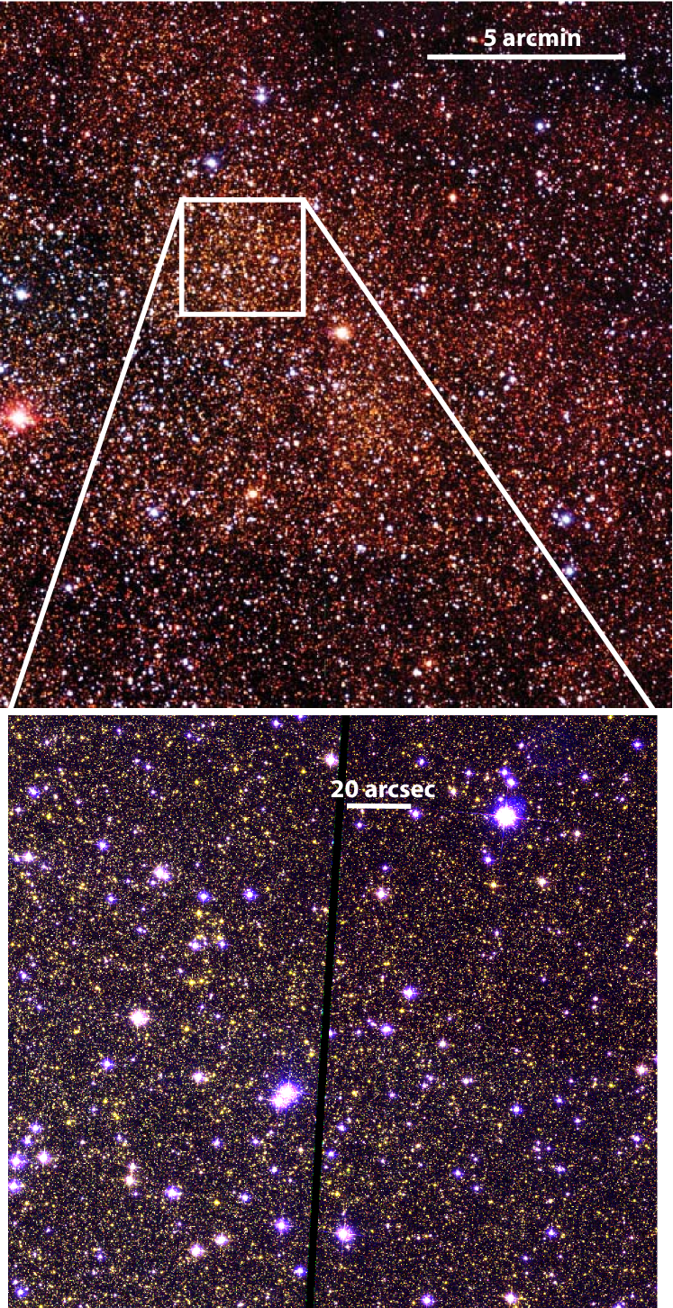
Figure 1: Three-color optical images of the field containing the ultra-deep Chandra observations of the CBF. The upper panel shows the mosaic image obtained by the 1.5m Russian-Turkish telescope (RTT150 telescope) (red shows the i’ spectral band, green - r’, blue - g’), while the lower panel shows a smaller area observed with the HST ACS/WFC (red - F625W, green - F658N, blue - F435W). From the top image it is evident that the interstellar extinction is strongly variable across the field (the regions close to boundaries of the figure are darker than the central regions). It is seen that the majority of stars are relatively faint and yellow – these are the old bulge population of the Galaxy.

In comparison with the Solar neighborhood, the analysis of the origin of the X-ray emission from the CBF has its own complications:

• First of all, we need to know the stellar density enclosed by the volume studied by Chandra.

• We need to understand the importance of the absorption that results from cold interstellar matter along the line of sight.

To study these issues, we used observations of the CBF in the optical band. In addition to the deep narrow-field images obtained with HST, large mosaics ($\sim 25^{\prime}\times 25^{\prime}$) of the field were obtained with the ground-based 1.5m Russian-Turkish telescope RTT150 (see Fig. 1) and the 6.5-m Magellan/Baade telescope (see Fig.2). In this paper we concentrate on the properties of the red clump giants (Sect. 2.1) in the CBF as derived from the HST images (Sect. 2.2) to infer properties of the interstellar extinction in this direction (Sect. 2.3) and constrain the stellar density distribution along the line of sight (Sects. 3.1 and 3.2). We also used results of the measurements with Spitzer/IRAC to compare the observed infrared emission towards the CBF with that predicted by the adopted stellar density model (Sect. 3.3). Our conclusions are summarized in Sect. 4. Other properties of the stellar population like age and metalicity will be explored in separate works. The ultimate goal, also to be addressed in a follow-up paper, is to derive the specific X-ray emission per unit mass and use this to study the unresolved X-ray emission from other galaxies.

2 Extinction in the CBF

2.1 Red clump giants

The red giant branch in the Hertzprung-Russell diagram shows a distinct feature that corresponds to a special subpopulation known as the red clump giants (RCGs). The intrinsic colors and absolute magnitudes of these core helium-burning stars are well-defined with little dispersion (e.g. Paczynski & Stanek 1998) and only a weak dependence on age and metallicity. Therefore RCGs can play the role of standard candles and are very useful for various studies of either stellar populations or properties of the interstellar medium. In particular, these stars have been used to map the Galactic bar (Stanek et al. 1994, 1997), to measure distances to the Galactic Center (Paczynski & Stanek 1998) and to the galaxy M31 (Stanek & Garnavich 1998), and to measure the properties (e.g. Wozniak & Stanek 1996) and spatial variations (Sumi 2004) of interstellar extinction in the Galactic bulge. Ground based observations with their limited angular resolution, encounter severe confusion problems in regions close to the Galactic Center (GC), which complicates the stellar photometry. Because of this problem and also due to the very large extinction, the majority of RCG studies were previously limited to angular distances larger than $\sim$2^∘ from the GC, while our field of interest is located at $\sim$1.5^∘ from the GC. As a demonstration of the confusion problems, we compare images of our field as observed by Magellan/IMACS with a seeing of 0.8″  and by HST ACS/WFC in Fig. 2. As the figure demonstrates, the ground based data are strongly confusion limited. Photometric measurements of stars with magnitudes fainter than $\sim 17-18$ are strongly affected by the contribution of fainter unresolved stars.

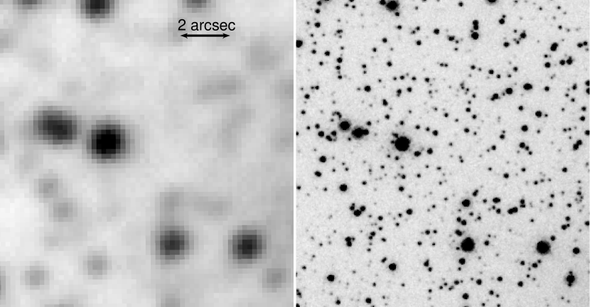
Figure 2: This comparison of a small part of the CBF as observed by Magellan/IMACS ($R$) (left) and the HST ACS/WFC (F625W) (right) demonstrates the problem of confusion in ground-based images.

2.2 Intrinsic properties of RCGs in the F435W and F625W filters

To understand the luminosity and intrinsic colors of an unabsorbed population of RCGs in the selected HST/ACS filters, we used the catalog of 284 Hipparcos RCGs from Alves (2000). As we are unable to make real observations of all listed RCGs in these two filters, we calculated their apparent brightnesses with the Kurucz model atmosphere spectra as included in the SYNPHOT/STSDAS/IRAF package (Bushouse & Simon 1994) as follows. For all stars in Table 1 of Alves (2000) we selected the stellar models that best match the combination of $B-V$ and $V-I$ colors as presented in Alves (2000). The resulting spectra were then convolved with the F435W and F625W transmission curves in SYNPHOT to calculate the magnitudes in these filters. We assumed that all stars in Alves (2000) have zero extinction, because they are all very nearby. As a check of the overall approach, we calculated the predicted magnitudes of the stars in the $K$ band and compared them with their observed $K$ magnitudes as listed in Alves (2000). The difference between the predicted and observed magnitudes has a normal distribution with zero mean and rms scatter of 0.13 mag, demonstrating that our approach is reasonable. We might expect that the accuracy of the predicted brightnesses in the F435W and F625W filters is even better because their transmissions are closer to those of the $B$, $V$ and $I$ filters—which we used as a reference for the spectral modeling—than to the $K$-band response.

Figure 3: Distribution of the absolute brightness of the 284 red clump giants in Table 1 of Alves (2000), converted into the F625W HST/ACS filter. The solid curve is the model fit to the distribution. It consists of a linear function plus a Gaussian with centroid at $M_{\rm F625W}=0.75$ and $\sigma=0.19$.

The resulting distribution of absolute magnitudes of RCGs in the F625W filter is presented in Fig. 3. The distribution is clearly peaked, with centroid at $M_{\rm F625W}=0.75$ and an rms scatter around this value of $0.19$. The solid line model includes also the linear component following the approach of Alves (2000), which reflects some ”background” population of red giants in the considered color and brightness intervals. The color of the peak of the RCG distribution is $\langle M_{\rm F435W}-M_{\rm F625W}\rangle=0.52$ with an rms scatter $0.18$. There is no strong indication for the dependence of the position of the peak on color.

As an additional check, we repeated the above analysis with the SYNPHOT spectra from the Pickles atlas (Pickles 1998) and found the same distribution for $M_{\rm F625W}$.

2.3 Ratio of the total-to-selective extinction

For our subsequent analysis, we used the HST/ACS images taken with the F435W and F625W filters, which are somewhat similar to the SDSS g’  and r’  filters, to identify the RCGs in the CBF and derive their magnitudes. Details of the photometric analysis are given in van den Berg, Hong, & Grindlay (2009). Below we will use the STMAG photometric system.

It has been shown by several authors that the extinction law towards the Galactic bulge differs from the standard one and in addition shows variations between different lines of sight (see e.g. Popowski 2000; Udalski 2003; Sumi 2004). Therefore we must determine the extinction law before we are able to determine the total extinction in our field. Like Udalski (2003) and Sumi (2004) we used the shift of the RCGs in the ($m_{\rm F625W}$, $m_{\rm F435W}-m_{\rm F625W}$) color-magnitude diagram due to variable extinction in our field to estimate the ratio of the total-to-selective extinction. This shift can be clearly seen in the spatially-resolved ($m_{\rm F625W}$, $m_{\rm F435W}-m_{\rm F625W}$) color-magnitude diagrams in Fig. 2 of van den Berg, Hong, & Grindlay (2009). Then, using the mean intrinsic color of RCGs as determined above, we calculated the total extinction towards the CBF.

Figure 4: Dependence of the mean magnitude of RCGs on their mean colors for different locations within the HST/ACS field. The slope of the linear fit to these positions (solid line) measures the ratio of the total to selective extinction $R_{\rm F625W,F435W}=1.25\pm 0.09$.

We divided the area observed by HST/ACS into rectangular bins of the size $0.96^{\prime}\times 0.96^{\prime}$. Of the stars detected in each angular bin we filtered out those that are clearly not associated with the red clump, viz. those that are fainter in F625W than $m_{\rm F625W}>17+(m_{\rm F435W}-m_{\rm F625W})$ and have a color $(m_{\rm F435W}-m_{\rm F625W})$ less than 2.0. To measure the mean magnitude and color of RCGs, we then determined the mean color and magnitude of the stars within an ellipse of the height $\Delta m_{\rm F625W}=0.5$ mag and width $\Delta(m_{\rm F435W}-m_{\rm F625W})=1$ mag which is centered on the peak of the number distribution of the remaining stars in the color-magnitude diagram. The resulting dependence of the mean magnitude of RCGs on their mean color is presented in Fig. 4. The variation of the RCG mean magnitude with color can be adequately described by a linear function with a ratio of the total-to-selective extinction $R_{\rm F625W,F435W}\equiv\Delta\langle m_{\rm F625W}\rangle/\Delta\langle m_{\rm F435W}-m_{\rm F625W}\rangle=1.25\pm 0.09$. The scatter of the measured centroids of the RCG positions around this fit is compatible with the statistical uncertainties in the individual centroids. The total number of RCGs used in these calculations is on the order of a few hundreds per $0.96^{\prime}\times 0.96^{\prime}$ bin. Note that the standard extinction law predicts $R_{\rm F625W,F435W}\approx 1.8-1.9$ (Sirianni et al. 2005), thus larger than we measure in the CBF (a similar conclusion regarding the smaller ratio of the total-to-selective extinction was found previously by e.g. Popowski 2000; Udalski 2003; Sumi 2004)

The position of the red clump in the color-magnitude diagrams of the two different spatial bins is shown in Fig. 5. A color-magnitude diagram of all photometered stars in the HST/ACS images with the extinction reduced to the value of $A_{\rm F625W}\sim 3.5$ is shown in Fig. 6.

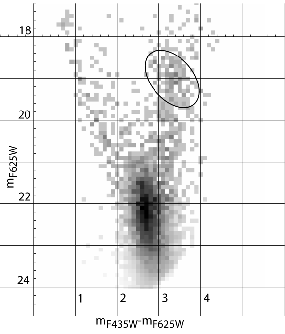
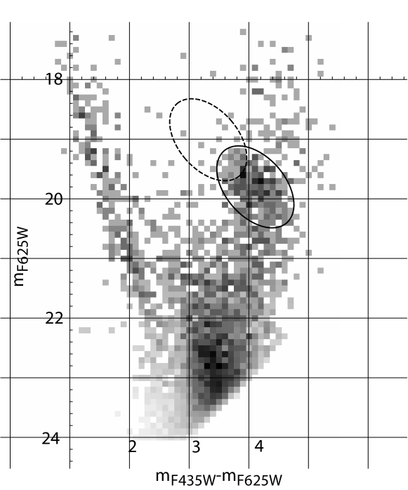
Figure 5: Color-magnitude diagrams in two areas of the HST/ACS field, with the number of stars per image bin color coded. The number of faint stars ($m_{\rm F625W}>20.5$) is artificially depressed via multiplication by a factor $\exp(-(m_{\rm F625W}-20.5)^{2}/3)$. The positions of the RCGs are marked with ellipses. In the lower panel, the ellipse with the dashed outline shows the position of the RCGs in the color-magnitude diagram of the upper panel. The ellipses are elongated in the direction of the reddening in the field; note that this direction is somewhat different from the one predicted by the standard extinction law, see text.

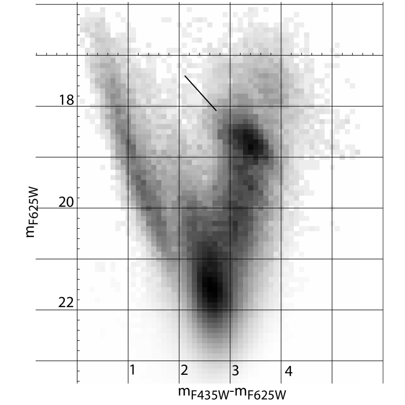
Figure 6: Color-magnitude diagram of all photometered stars in the HST/ACS field. The magnitudes and colors of stars in each rectangular $0.96^{\prime}\times 0.96^{\prime}$ bin are extinction corrected to the value $A_{\rm F625W}\sim 3.5$. The number of faint stars ($m_{\rm F625W}>19.5$) is artificially depressed via multiplication by a factor $\exp(-(m_{\rm F625W}-19.5)^{2}/2)$. The line shows the direction of the reddening. The number of stars per image bin is color coded.

Now we computed the apparent magnitude of RCGs corrected for extinction ($m_{\rm F625W,0}$) in each spatial bin with the assumption that their intrinsic mean color is $\langle m_{\rm F435W}-m_{\rm F625W}\rangle_{0}=0.52$:

$$\langle m_{\rm F625W}\rangle=m_{\rm F625W,0}+R_{\rm F625W,F435W}\times$$

$$(\langle m_{\rm F435W}-m_{\rm F625W}\rangle-\langle m_{\rm F435W}-m_{\rm F625W}\rangle_{0}).$$

The resulting average value is $\langle m_{\rm F625W,0}\rangle=15.4\pm 0.3$. This allows us to make an estimate of the effective distance to the location of the majority of the RCGs. The resulting distance modulus is $m-M=14.7\pm 0.3$, which translates into a distance $D=8.7\pm 0.9$ kpc, in agreement with recent distance estimates to the Galactic Center (Eisenhauer et al. 2005; Ghez et al. 2008). The average extinction in the HST/ACS field is $A_{F625W}\sim 4$ and the extinction ranges from $\sim 3$ to $\sim 5$.

3 Constraints on the stellar density distribution in the CBF

The shape of the clump formed by the RCGs in Fig. 6 suggests that their position is still affected by additional extinction – the distribution of the RCGs appears a bit elongated in the direction of the reddening. This shows that the extinction varies even on angular scales smaller than $0.96^{\prime}$. Note that this effect is almost absent in regions with smaller total extinction – after correction for extinction, the RCGs form a quite compact locus without an extension in the reddening direction (see e.g. Sumi 2004).

However, apart from the possible elongation connected with any residual reddening effects, the RCGs define a relatively narrow clump, which can be used to constrain the distribution of stars along the line of sight toward the CBF.

3.1 Model of the stellar distribution

In any direction within the Galaxy stars are distributed over a range of distances along the line of sight. In the regions far away from the GC, the dominant stellar component is the stellar disk, while at small angular distances from the GC the majority of the stellar mass is provided by the Galactic bulge and/or bar, nuclear stellar disk or nuclear stellar cluster components. In our subsequent analysis we will consider only three components of the stellar distribution: the Galactic bulge, Galactic disk and nuclear stellar disk. We will adopt the distance to the Galactic Center of 8 kpc, which is some intermediate value between measurements of Eisenhauer et al. (2005) and Ghez et al. (2008). The nuclear stellar cluster is important only for the very central parts of the Galaxy, at distances less than 10–20 arcmin (see e.g. Launhardt, Zylka, & Mezger 2002), and, therefore we will not consider it here. We use the following simplified models of the three stellar components. Here $r$ is the Galactocentric distance, $z$ is the height above the Galactic plane.

For the stellar disk density we use (from Revnivtsev et al. 2006)

$$\rho_{\rm disk}=2.5\leavevmode\nobreak\ {\rm M_{\odot}\leavevmode\nobreak\ pc^{-3}}\times$$

$$\exp(-(3.0{\rm kpc}/r)^{3}-(r/2.5{\rm kpc})-|z/130{\rm pc}|).$$

The normalization of this component was chosen to yield an integrated stellar disk of $10^{10}\leavevmode\nobreak\ M_{\odot}$, which is approximately equivalent to the measured stellar density in the solar neighborhood ($0.045M_{\odot}$ pc^-3, e.g. Robin et al. 2003). As we will see below, details of the stellar disk model are not important because of its small contribution to the total mass budget in the CBF.

For the Galactic bulge component we used the simple analytic form from Dehnen & Binney (1998) and Grimm, Gilfanov, & Sunyaev (2002)

$$\rho_{\rm bulge}=1.09\leavevmode\nobreak\ {\rm M_{\odot}\leavevmode\nobreak\ pc^{-3}}\left({\sqrt{r^{2}+(z/0.6)^{2}}}\over{1{\rm kpc}}\right)^{-1.8}\times$$

$$\exp\left(-{{r^{2}+(z/0.6)^{2}}\over{1.9{\rm kpc}^{2}}}\right).$$

The adopted total mass of the Galactic bulge is $1.3\times 10^{10}\leavevmode\nobreak\ M_{\odot}$ (Dwek et al. 1995).

We assumed that the nuclear stellar disk (NSD) has the following density distribution

$$\rho_{\rm NSD}=\rho_{d}r^{-\alpha}e^{-|z|/0.045{\rm kpc}},$$

where $\rho_{d}=300M_{\odot}$ pc^-3. At $r<0.12$ kpc, the slope $\alpha=0.1$, at $0.12$ kpc $<r<0.22$ kpc, $\alpha=3.5$, and at $r>0.22$ kpc, $\alpha=10$ (Launhardt, Zylka, & Mezger 2002). The total mass of the NSD is thus $1.4\times 10^{9}M_{\odot}$. In reality this quantity is uncertain by about 50% (Launhardt, Zylka, & Mezger 2002).

The resulting assumed distribution of the stellar density along the line of sight in the direction of the CBF is presented in Fig. 7. For the adopted model, the total surface mass density in this direction is $4.6\times 10^{4}\leavevmode\nobreak\ M_{\odot}$ sq.arcmin^-1, while the bulge component contributes $3.9\times 10^{4}\leavevmode\nobreak\ M_{\odot}$ sq.arcmin^-1, the stellar disk contributes $2.3\times 10^{3}\leavevmode\nobreak\ M_{\odot}$ sq.arcmin^-1, and the nuclear stellar disk contributes $4.2\times 10^{3}\leavevmode\nobreak\ M_{\odot}$ sq.arcmin^-1.

Figure 7: Distribution of the density in the different adopted stellar Galactic components along the line of sight in the direction of the CBF, i.e. towards $(l^{II},b^{II})=(0.1^{\circ},-1.42^{\circ})$.

3.2 Comparing the shape of the stellar model distribution with HST observations

By choosing some fiducial number of the RCGs per unit mass of the stellar population, we can use these stellar distribution models together with the intrinsic magnitude distribution of RCGs (Fig. 3) and the derived extinction in our field, to construct the differential distribution of RCGs as a function of their apparent magnitude in the F625W band and compare this prediction with the data. The model distribution and the observations (distribution of photometered stars from Fig. 6 with colors $m_{rmF435W}-m_{\rm F625W}>2.5$) are shown in Fig. 8. Here we assumed that all (or the majority of) stars are located behind the extinction region. This assumption is supported by studies of the distribution of the interstellar extinction along the line of sight by e.g. Drimmel, Cabrera-Lavers, & López-Corredoira (2003) or Marshall et al. (2006). See also Fig. 1 in van den Berg, Hong, & Grindlay (2009), which shows that according to these models most of the absorbing material is closer than $\sim$6 kpc, whereas Fig. 7 in this paper shows that the bulk of stars lies further away than $\sim$6 kpc.

Figure 8: Crosses - observed differential distribution of the number of stars in the HST/ACS field with color $m_{\rm F435W}-m_{\rm F625W}>2.5$ as a function of their apparent F625W magnitude after correcting all magnitudes to a common value of the extinction that corresponds to some arbitrary chosen position in the field of view (see color-magnitude diagram on Fig. 6). The size of the magnitude bins is 0.085 mag. Solid histogram - modeled differential distribution of RCGs as a function of their apparent F625W magnitude in the field of our study. The dashed line shows a part of the same distribution but with some linear function added to match the surrounding magnitude bins.

Figure  8 shows the model distribution of stars in the studied region (histogram and dashed line). It was obtained via convolution of the model of the stellar mass distribution over the line of sight with the distribution (see Fig.7) of RCGs over their absolute magnitudes (see Fig.3), assuming the denisty of the RCGs in their gaussian component $N_{\rm RCG}/M_{*}\sim 1.6\times 10^{-3}\leavevmode\nobreak\ M^{-1}_{\odot}$. This normalization value was chosen to fit the observed points. This RCG density number in general looks reasonable (see e.g. López-Corredoira et al. 2002), however, a more quantitative comparison of this number with those obtained in different observational and theoretical works requires more accurate treating of different selection effects. The figure shows that the model distribution very closely follows the measured points (crosses) around the corresponding peak of the color-magnitude diagram. The linear function that is added to make the model distribution match with the magnitude bins that surround the observed peak could originate from red giants and asymptotic giant branch stars that also lie in this part of the color-magnitude diagram, but do not belong to the red clump (see also Alves 2000).

There are some other subtle differences to note. In particular, the model (which takes into account the intrinsic dispersion of the RCGs brightnesses at the level of $0.19$ mag) has a Gaussian width of the main peak of $0.23$ mag. However, the Gaussian width of the RCG peak is $0.28\pm 0.01$ in the CBF. This is somewhat higher than we might expect from our model.

We should keep in mind though that there may be several complications that could result in the observed additional broadening. For example, it is likely that we have not completely corrected for all the extinction in our field due to its variations on small angular scales (see the discussion of the shape of the red clump in Fig. 6); with the adopted technique based on RCGs, these variations are difficult to account for, because the density of RCGs is too low to use smaller spatial bins. Residual variations of the total extinction in our field with an amplitude $\Delta A_{\rm F625W}\sim 0.16$ mag can result in the observed broadening of the RCG distribution.

It is also possible that the intrinsic (i.e. approximately extinction-corrected) brightness of the RCGs in the Galactic bulge has a slightly higher scatter than that in the Solar vicinity, which we used to compute the model distribution.

It is also possible that the extra broadening is the result of our oversimplified picture that all the extinction is located in front of the majority of the Galactic bulge RCGs. If some residual extinction, distributed within the Galactic bulge, is present in our field, it will similarly result in a slight widening of the RCG peak in the differential number-counts plot.

Finally it could be that the adopted model for the stellar density distribution of the bulge oversimplifies the true distribution, resulting in a density peak that is too narrow. However, our tests to vary the parameters of the stellar model showed that the latter is unlikely.

Summarizing the above findings, we conclude that the shape of the adopted model of the stellar density distribution in the Galaxy adequately describes the observed distribution in the CBF.

3.3 Stellar surface brightness in the near-infrared

Another important check of the adopted stellar mass distribution in the direction of the CBF is the total surface brightness provided by stars. We took the value of the total luminosity density of the Galactic bulge as measured by Dwek et al. (1995) at a wavelength 3.5 $\mu$m – $4.19\times 10^{28}$ erg s^-1 Hz^-1 – and assigned it to our adopted total mass of stars in the Galactic bulge – $1.3\times 10^{10}\leavevmode\nobreak\ M_{\odot}$ – to calculate a specific infrared luminosity density per unit mass. Then we integrated the surface brightness provided by all stars in our model (assuming the same luminosity-to-mass ratio for all stellar components). We point out that due to differences in age and/or composition compared to the bulge, the true specific luminosity density at 3.5 $\mu$m could be slightly different for the (nuclear) disk, although their contributions to the total surface brightness are relatively small (see below). The result of this integration is shown in Fig. 9. The observed infrared surface brightness at 3.6 $\mu$m in our field is $21\pm 2$ MJy/sr, or $1.78\pm 0.18$ Jy sq.arcmin^-1, as measured by Spitzer/IRAC (see Revnivtsev et al. 2009). It is seen that the adopted model correctly predicts the observed surface brightness. The majority of the 3.5 $\mu$m flux is provided by the stellar population in the Galactic bulge ($\sim$82%) with small contributions from the stellar disk ($\sim$9%) and the nuclear stellar disk ($\sim$9%). The dominance of the Galactic bulge stars to the total stellar mass budget in the field is also evident from Fig. 1. The vast majority of stars in the high resolution HST/ACS image are faint and have a yellow/red color, which shows that they are of a relatively low mass and are located at a large distance from us. This is exactly what is expected for a stellar population of the Galactic bulge with an age of $\sim$10 Gyr.

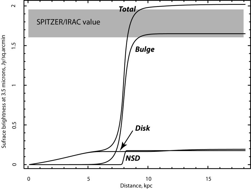
Figure 9: Cumulative stellar surface brightness at 3.5 $\mu$m in the direction of the CBF as predicted by the adopted stellar mass model, decomposed in the three components (“Bulge”, “Disk” and “NSD”) as well as their total. The measured surface brightness as measured by Spitzer/IRAC at 3.6 $\mu$m is shown by the gray area.

4 Conclusions

The study of populations of Galactic X-ray sources requires knowledge of the properties of the underlying population of normal stars, because only then one can estimate the statistical properties of X-ray sources and their systematic dependencies on the age, metallicity, density etc. of the stellar population. One of the largest projects performed recently by the Chandra X-ray Observatory is the ultra-deep observation of a region close to the Galactic Center - the CBF. This observation provides us with a wealth of data on the X-ray population in this area. To connect these properties to the properties of normal stars we must study this area in the optical and near-infrared bands.

We analyzed HST/ACS images of the central 6.6′$\times$ 6.6′  field of the CBF in the F435W and F625W bands and found the following:

• Interstellar extinction in the direction of the CBF is $\langle A_{\rm F625W}\rangle\sim 4$ and variable on an angular scale of $\sim$1′. Variations of the extinction in this area on larger scales were previously noticed by Dutra et al. (2003) ($4^{\prime}$ scales), Revnivtsev, Burenin, & Sazonov (2009) ($1.8^{\prime}$ scales), van den Berg, Hong, & Grindlay (2009) ($1.6^{\prime}\times 3.2^{\prime}$ scales).

• The color-magnitude diagram corrected for extinction, as determined in angular bins of $0.96^{\prime}\times 0.96^{\prime}$, suggests that there is still residual extinction on smaller scales at the level of $A_{\rm F625W}\sim 0.2$ mag or less. This would be difficult to measure with RCGs due to their decreasing numbers.

• We determined the extinction law (in particular, the ratio of the total-to-selective extinction $\Delta\langle m_{\rm F625W}\rangle/\Delta\langle m_{\rm F435W}-m_{\rm F625W}\rangle$) in the direction of the CBF – $1.3\pm 0.1$ – and found that it is significantly different from the canonical one $\sim 1.9$. The discrepancy shows a similar trend as that determined by various authors using OGLE data of the bulge (e.g. Popowski 2000; Udalski 2003; Sumi 2004). This suggests that we might expect deviations from the standard correspondence between the photoabsorption column $n_{H}L$, measurable in the X-ray band, and extinction in the optical/NIR bands. This likely differing X-ray (vs. IR) absorption in the bulge region will affect derived intrinsic X-ray spectra and thus (in some cases) the inferred source types (e.g., with less X-ray absorption for a given color excess, soft spectral components will be decreased, etc.).

• We compared a model of the stellar distribution along the line of sight towards the CBF with the observed distribution of red clump giants in the color-magnitude diagram. We show that the adopted model adequately describes the data. In the model, the majority of the stellar mass in the direction of the CBF is provided by Galactic bulge stars with only a small contribution from the stellar disk and nuclear stellar disk components ($\sim 5$% and $\sim$9%, respectively). Small discrepancies between the model and the data could be the result of variations in the extinction on small angular scales ($\lesssim$1′), differences between the local and bulge luminosity functions of red clump giants, uncertainties in the distribution of the extinction along the line of sight, or an oversimplified model of the stellar mass profile of the bulge.

• We showed that the adopted stellar model predicts an integrated 3.5 $\mu$m surface brightness of this part of the Galaxy that is only 13% higher than the surface brightness actually measured by Spitzer/IRAC in the 3.6 $\mu$m band.