Tempo and Mode of Evolution in the Tangled Nature Model

Abstract

We study the Tangled Nature model of macro evolution and demonstrate that the co-evolutionary dynamics produces an increasingly correlated core of well occupied types. At the same time the entire configuration of types becomes increasing de-correlated. This finding is related to ecosystem evolution. The systems level dynamics of the model is subordinated to intermittent transitions between meta-stable states. We improve on previous studies of the statistics of the transition times and show that the fluctuations in the offspring probability decreases with number of transitions. The longtime adaptation, as seen by an increasing population size is demonstrated to be related to the convexity of the offspring probability. We explain how the models behaviour is a mathematical reflection of Darwin’s concept of adaptation of profitable variations.

I Motivation

In his 1944 book Simpson1944 , Simpson’s expressed aim was to reconcile the fruits of paleontological research with the Darwinian synthesis. The Darwinian synthesis, such as it was, consisted of Darwin’s original ideas concerning competition for scarce resources and natural selection married to more recent discoveries revealing the first genetic, then fundamentally molecular, mechanisms by which Darwin’s ideas were realised. The question that Simpson wanted to answer was: is it possible to infer anything about the mode of evolution simply by observing its tempo.

The point, that has been made in different ways since Simpson’s seminal work, is that, as Simpson has it, and as Gould has subsequently underlined Gould1995 , what holds for ten rats over a hundred years may not be true, or may not be simply extrapolated, to a million rats over a billion years. In this paper, we take this point further, by observing the tempo of evolution of a model of interacting populations of different species. We find that there are two separate dynamical regimes on which evolution takes place. In one of those, the tempo gradually decelerates due to the frustration in the interactions between different species. In the other, observable quantities fluctuate around stationary values.

A related issue is whether evolutionary dynamics on all spatial scales, ranging from bacterial colonies confined in a flask (see eg. Lenski2008 ) to biological species can be understood, at least in an approximate fashion, using a small set of unifying theoretical principles. These principles would explain the emergent properties of evolutionary systems, for example the decrease of the rate of evolutionary events on coarse-grained time scales Raup1982 , in spite of the microscopic rate of change remaining constant. Clearly, evolution at the collective level is a non-stationary process, characterised by various trends. How are these trends related to the dynamics at the level of individuals? .

An approach which has gained momentum due to the increasing speed and availability of computers, is to search for unifying principles by simulating simple evolutionary models with Monte Carlo techniques. These models blend a random element, the noise, with deterministic rules for the average rates of reproduction, mutation and death in a group or groups of individuals. Precursors to our approach include Kauffman’s NK(C) model, which has been used primarily as a tool to study the way fitness landscapes affect the course of evolution Kauffman1990 . Our approach, while partially derived from the NKC model, is different in two ways: we have frequency dependent interaction, and we do not explicitly build in a optimisation. The fact that our model nevertheless appears to optimise certain macroscopic parameters is a matter of some interest, and is discussed further below.

There are many elements of the puzzle that we will simply neglect. Indeed the model we shall study does not even have the rudimentary innovation of sexual reproduction. This approach, we should make clear, is limited and cannot provide a complete answer to the question of how the microscopic and macroscopic are related. However, we show that even such a simple model as the one discussed can give rise to macroscopic evolution of a very different tempo from the individual dynamics on which it is based, and we show how this emergent macroscopic behaviour comes about from the interaction of many individuals following Darwinian principles. It is the glassy nature of evolutionary dynamics - the existence of quenched disorder giving rise to slow relaxation - that in our model produces the macroscopic tempo of a different nature from that of the underlying dynamics.

II The Microscopic Level

The Tangled Nature model of co-evolution Christ2002 has already been studied in several contexts. Its simplicity along with the rich complexity of its resulting behaviour makes it a paradigmatic model for testing co-evolutionary ideas. The model retains the binary string genotype geometry found in previous approaches, but replaces their ‘ad hoc’ static fitness landscapes with a set of population dependent interactions between extant species, similar to the ‘tangled’ interactions of an eco-system. This simple addition creates a fascinating complex behaviour: the model retains the intermittent dynamics found for adaptive walks in fitness landscapesSibani99a, where periods of quasi-stasis which are long with respect to the timescale of the underlying, reproductive dynamics, are interspersed by transition events, termed quakes, which occur at a decreasing rate. The overall tempo of evolution is decelerating in the model, indicating the possibility of an underlying process optimising a hidden variable. Importantly, the model introduces new, and biologically relevant, variables in the dynamics at the macroscopic level. As the system evolves from a ‘random’ initial state in the presence of scarce external resources, the network of extant and interacting population changes, slowly, but radically over time, enabling the system to support an ever growing number of individuals in the face of a constant supply of external resources.

Despite its simplicity, the model is able to reproduce the long time decrease reported in the overall macroscopic extinction rate, the observed intermittent nature of macro-evolution, denoted punctuated equilibrium by Gould and Eldrdege Gould1977 , the log-normal shape often observed for the species abundance distributions Anderson2004 , the power law relation often seen between area and the number of different species number Jensen2006 , the frame work of the model is also able to reproduce often reported exponential degree distributions of the network of species as well as the decreasing connectance with increasing species diversity that has attracted much observational and theoretical interest Laird2007 .

Individuals are defined by a binary string of length $L$, and are thus points in an $L$ dimensional hypercube, whose elements, or nodes, will be denoted by Latin letters $i$ and $j$. An a priori given fixed and random matrix $J_{ij}$, specifies the strength and type of potential interaction between populations at nodes $i$ and $j$. The evolutionary dynamics of the model, to be explained in detail below, leads to the occupancy of types evolving with time. Mutation allows new nodes to become inhabited and existing occupied types to go extinct. The configuration of occupied types changes accordingly with time. Although the dynamics at the level of individuals is smooth and always happens at the same rate, at the systems level, i.e. the level of occupied configurations in type space, the dynamics is highly intermittent, and, as mentioned, decelerating. The dynamics of the model is characterised by a succession of quasi stable states (or QESS: quasi evolutionary stable strategy). Each QESS is described by a network of sites which are populated and interact with each other. As the system undergoes the intermittent burst of changes to the occupancy one network of occupied sites is replaced by another.

The long time evolution of the occupancy in type space, and all the properties that can be derived form the composition and interactions of the extant population, are subordinated to the transitions, or the quakes, as they are customarily denoted in record dynamics. This is because no essential change occurs during the metastable state. The occupancy of individual sites may fluctuate but, since essentially the same set of types are present during the metastable periods, no net drift can manifest itself. The most conspicuous overall effect of the succession of QESS is a logarithmically slow increase in the overall population size.

The evolution of the configuration in type space is non-stationary nature and the population grows logarithmically with time as the configurations, through the adaptive search that takes place during the quakes events, manage to become collectively better adapted. The adaptation consists in selecting networks of occupied sites in type space connected by increasingly mutualistic or beneficial interactions, which enables the temporal averaged net-reproduction rate to slightly overcome the killing rate.

A time-step in the model is carried out as follows: an individual is picked at random. Its offspring probability is calculated by first calculating the value of

$$H=\frac{C}{N}\sum_{j}J_{ij}n_{j}-\mu N$$

where N is the total population, $n_{j}$ the site populations, $C$ a strength parameter and $\mu$ the carrying capacity determining the resources available to the population. This value is then mapped on to the interval 0,1 using the function

$$P_{off}=\frac{1}{1+\exp(-H)},$$

which is the probability of reproduction in that time step. Reproduction is asexual: the parent is replaced by two copies of itself, with each offspring susceptible to mutations with probability $p_{mut}$ per genome site. In the next step a randomly chosen individual is killed with constant probability $p_{kill}$. Note that while a point mutation creates a new individual on a neighboring site of the hypercube on which populatons reside, the interaction matrix generally involves populations located at arbitrary positons on the hypercube.

Typically the population is initially located on a randomly chosen, single site. To start with, the population decreases. Then, as reproduction becomes more likely, mutants begin to populate neighbouring sites. Soon a stable “ecosystem” is formed, a subset of genotypes whose mutual interactions form a (meta)stable dynamical system. This subsystem can be characterised by some key macroscopic properties - the average total number of individuals in the system, the average number of sites occupied, and the properties of the realised interaction network.

III The Macroscopic Level

III.1 Centre of mass

Since the system is made up of weighted nodes (each with a vector position in genotype space) interacting with each other, we can define a quantity analogous to the centre of mass in classical mechanics. We define this as the species occupancy weighted average position of the system in genotype space, $\mathbb{A}$, where

$$\mathbb{A}=\frac{1}{N}\sum_{j}n_{j}\mathbb{s}_{j}$$ (1)

where $\mathbb{s}_{j}$ denotes the position of vertex number $j=1,...,2^{L}$ in the $L$ dimensional hypercube of genotypes, $n_{j}$ is the occupancy of species $j$ located at vertex $\mathbb{s}_{j}$ and $N$ is the total population: ($N=\sum_{j}n_{j}$).

During meta-stable periods this quantity remains practically constant, since it is only slightly modified by population fluctuations, which chiefly occur on the periphery of the system due to mutations. In contrast, when a quake occurs the centre of mass undergoes a major displacement. While it may be theoretically possible that a quake would occur which does not shift the centre of mass perceptibly, this is highly unlikely since any nearby stable configuration would undermine the stability of the current configuration.

Figure 1: The time evolution for a typical run of the Tangled Nature model. The diversity (blue) displays intermittent behaviour, exhibiting long plateaux interspersed with chaotic fluctuations (the diversity counts the number of species in the system, and behaves in much the same way as the population). The change in centre of the mass of the system (red) follows the same pattern - in general there is very little movement, with occasional big leaps in position.

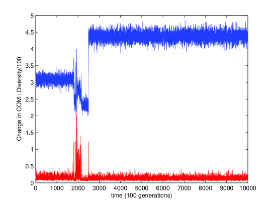
The CM then unambiguously identifies significant rearrangements in genotype space. In what follows, monitoring the CM position allows us to explore how the tempo of such rearrangements evolves with the age of the system, counted from the beginning of the simulation..

Figure 1 plots the changes in this quantity, with a plot of the total population for reference. Importantly we see that both variables exhibit the same behaviour, and it follows that one can be used as a good proxy for the other. In what follows we analyse population increments as a proxy for the underlying shift in configuration, since this is much more computationally efficient.

III.2 Aging

There are two distinct tempos in the dynamics of the model, as has been suggested in previous papers. The nature of these two tempos is investigated here. Figure 1 gives a qualitative picture of their origin - we see that the dynamics can be broadly divided into chaotic and stable phases, with the stable phases tending to be long-lived, as opposed to the chaotic phases which tend to be brief interludes. Within the stable phases there is still some dynamics due to the stochastic nature of the system: fluctuations and sometimes natural cycles around a fixed point are observed. Thus, there are two obvious timescales in the system - one governing the fluctuations within each stable phase, the other the chaotic transitions between stable phases.

To determine the tempo of these phases, or more precisely to determine how the frequency of these two types of events scale with the age of the system we use a technique borrowed from analysis of spin glasses Sibani:2003p22 ; Sibani07 . In spin glasses the thermally activated evolution can be analyzed by constructing the Probability Density Function (PDF) of the heat flow between the system and its thermal reservoir. Large, irreversible flows of heat out of the system only occur when the system undergoes a significant rearrangement, or quake. Consequently, observing how the PDF evolves over time reveals how the tempo of reversible and irreversible events evolve over time. In our case, an exact equivalent of the energy in a spin glass is not available. Instead, we choose a characteristic scalar function of the dynamics, the population. In spin glasses the energy has a much more well defined role in the dynamics than does the population in the Tangled Nature model -possible changes in configuration are namely accepted or rejected based on energetic considerations, whereas the population plays no such discriminatory role in the present model.

Letting $t_{w}$ be the age of the system, we consider the distribution of population increments

$$N(t_{w}+k\Delta t)-N(t_{w}+(k-1)\Delta t),$$

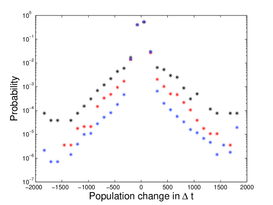
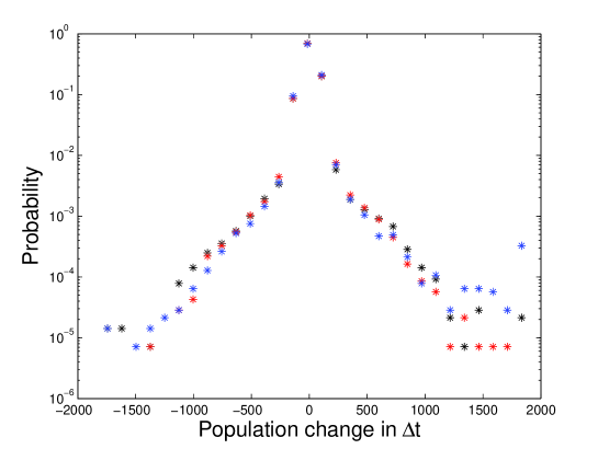
where $k=1,2,3,...,\frac{t_{w}}{\Delta tK}$, i.e. at different epochs in the system’s evolution over the observation interval $[t_{w},t_{w}+\frac{t_{w}}{K}]$, . The nature of the PDF will be determined by three parameters - $t_{w}$, $K$ and $\Delta t$. The first quantity, $t_{w}$, measures as mentioned the age of the system, while $K$ is inversely proportional to the size of the observation window. The last parameter is the number of Monte Carlo sweeps between consecutive measurements of the population size. We need the observation window to be large enough to capture both the quasi-equilibrium and non-equilibrium dynamics, while not being so long that the system changes too significantly over the window. In practice this is a matter of trial and error. In figures 2 and 3 the PDF of the population fluctuations is plotted for three different epochs, with $t_{w}=1000,10000,100000$ and $K=4$. The data comes from an ensemble of 1500 runs.

Figure 2 shows the data with $\Delta t=10$ for all epochs.The first thing to note is that the PDF has the characteristic shape common to similar spin glass studies, with one important difference. Since the data is plotted on linear-log axes, the parabolic shape in the centre represents a gaussian distribution, and the straight tails are exponential. The difference from the spin glass case is that here we have both positive and negative tails, whereas a in the heat flow PDF for a spin glass the positive tail is undetectable, corresponding to the fact that quakes reduce the energy of the system. The population, on the other hand, may go up or down in a quake, although, as we shall see, there is still an overall tendency for the population to increase.

In analogy with spin glasses, we identify the large, rare events in the tails with the irreversible quakes in the system. We see that as the system ages, these quakes become less and less frequent while the gaussian peak remains unchanged. We quantify this observation by rescaling the data - we anticipate a logarithmic decrease in the quake frequency, and so we make $\Delta t$ proportional to the age of the system. When we do this, the PDF from three different ages collapses on to a single curve, so that the probability of large fluctuations (that is fluctuations appearing in the exponential tails) must scale as $t_{w}^{-1}$, since the probability of a large fluctuation in time $\Delta t$ is to leading order $\Delta tP(t_{w})$, where $P(t_{w})$ is the probability of a large fluctuation as a function of $t_{w}$.

Figure 2: The PDF of population increments for an ensemble of 1500 runs of $10^{6}$ generations. Black: $t_{w}=1000$, red $t_{w}=10000$, blue $t_{w}=100000$. In this plot $\Delta t=10$. The older the system, the less probable a large population fluctuation becomes.

Figure 3: The PDF of population increments for an ensemble of 1500 runs of $10^{6}$ generations. Black: $t_{w}=1000$, red $t_{w}=10000$, blue $t_{w}=100000$. The total number of data points is equal for each age of the system; that is the sampling period $\Delta t=\frac{t_{w}}{100}$ scales with the age of the system. The data collapses onto a single curve, showing that the probability of a large fluctuation scales like $\frac{1}{t_{w}}$

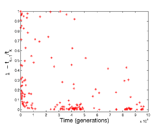
The waiting time distribution for quakes (figure 4) shows that the ratio of waiting time to age of the system remains non zero right throughout a million generation run, giving further proof that the quake probability decays with the age of the system.

Figure 4: Plot of a sample of quake waiting time ratios, where $t_{k}$ is the time of the $k^{th}$ quake. A Poisson distribution of quakes would give a more or less zero for long times, since the ratio would decay as $\frac{1}{\lambda t}$ for some average rate $\lambda$. Instead we see many non zero points for long times. The clustering of points along the $t$ axis is due to small ’secondary quakes’ that are hard to distinguish from primary quakes.

IV Discussion

We have shown that by studying the tempo of the evolution in a schematic model we can infer a great deal about the mode - broadly speaking we find that we can split the dynamics into two bits, one quasi-equilibrium and the other non-equilibrium relaxation. Here we would like to suggest a mechanism for the observed slowing down of the dynamics at the macroscopic scale. First, let us recall the work done in spin glasses on similar aging phenomena. It has been found there that many microscopically different systems can be modelled by a unifying mesoscopic principle of barrier hopping. In this picture the system becomes increasing stable against quakes as each quake corresponds to the jumping of a barrier in the energy landscape which is marginally larger than the barrier corresponding to the previous quake. Consequently, the evolution of the system is well described by record dynamics - each new maximum energy leads to a change in configuration and a new energy minimum. The energy landscape is such (for more detailed discussion see Sibani:1998p8 ) that each new well is deeper than the previous one, so the relaxation of the system slows as records become less and less frequent.

We propose that the similar relaxation dynamics seen in the Tangled Nature model is due to a similar scenario, with some caveats. One way of interpreting the spin glass dynamics is that the system falls into wells of increasing depth, from which it becomes increasingly hard to escape since the magnitude of the fluctuations of the energy about each new fixed point remains constant. In the tangled nature model, it is harder to justify an energy landscape picture, but we can measure the magnitude of fluctuations of the birthrate, which is a measure of the systems ability to ‘break out’ from each equilibrium state. To do this we have determined the standard deviation of the birth rate as a function of the age of the system, sampled during the different equilibrium stages of the dynamics. Indeed we find that there is a significant decrease in the fluctuation width over a simulation of $10^{6}$ generations.

To complete the circle, we also need to understand why a decrease in the birthrate probability fluctuations in turn leads to greater stability. A spike in the reproduction probability of the system has an effect beyond simple increase in numbers - it also increases the likelihood that new species in different parts of genotype space, generated by mutations, will interact and thus destabilise the current configuration. It should be emphasised that the difference between the fluctuations in the average probability and the fluctuations of the population amount to a difference in the weighting of the core and the periphery of the system - that is between between vital, heavily populated genotypes and transient, sparsely populated ones. When considering the birthrate, each site is weighted equally - so the fact that we see a decrease in these fluctuations while seeing a constant standard deviation in the population is not contradictory - it merely shows that the fluctuations are increasingly limited to sites, which are gradually becoming more similar in terms of the network of interactions $J_{ij}$ surrounding the sites carrying the larger proportion of the population.

Figure 5: The standard deviation of birth rate fluctuations decreases over time. The window index, $x$, gives the start and end points of each sample window using the following conversion: $t_{\small{start}}=10\cdot 2^{x}$ and $t_{\small{end}}=18\cdot 2^{x}$. Error bars show that while the effect is small, it is significant.

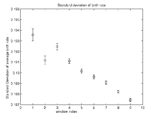
Figure 5 shows the decrease in the standard deviation of these fluctuations plotted over logarithmically spaced time intervals. The fluctuations were only measured in the metastable parts of the dynamics. This suggests that the system evolves in such a way that barrier hopping becomes less and less likely, not because of an increase in barrier height, but due to a decrease in the width of the fluctuations in the system.

This is not the end of the story, since these fluctuations are themselves governed by the nature of the network of interactions. Why the systems chooses configurations less susceptible to fluctuations has not been answered in this paper, and will form the focus of future work.

Acknowledgement: HJJ and DJ gratefully acknowledge the EPSRC for funding under grant EP/D051223

References

- (1) G. Simpson. Tempo and Mode in Evolution. Columbia University Press, 1944.
- (2) S. Gould. Tempo and mode in the macroevolutionary reconstruction of darwinism. In W. Fitch and F. Ayala, editors, Tempo and Mode in Evolution: Genetics and Palaeontology 50 years after Simpson. National Academy Press, 1995.
- (3) Zachary D. Blount, Christina Z. Borland, and Richard E. Lenski. Historical contingency and the evolution of a key innovation in an experimental population of escherichia coli. PNAS, 105(23):7899–7906, 2008.
- (4) D. Raup and J. Sepkoski Jr. Mass extinctions in the marine fossil record. Science, 215:1501, 1982.
- (5) Stuart A. Kauffman. The Origins of Order: Self Organisation and Selection in Evolution. Oxford University Press, 1990.
- (6) Kim Christensen, Simone A. Di Collobiano, Matt Hall, and Henrik J. Jensen. Tangled nature: A model of evolutionary ecology. Journal of Theoretical Biology, 216(1):73 – 84, 2002.
- (7) P. Sibani and A. Pedersen. Evolution dynamics in terraced NK landscapes. EuropPhysics Letters, 48:346–352, 1999.
- (8) Steven J. Gould and Niles Eldredge. Punctuated equillibria; the tempo and mode of evolution reconsidered. Paleobiology, 3:115, 1977.
- (9) Paul Anderson, Henrik J. Jensen, L Oliveira, and Paolo Sibani. Evolution in complex systems. Complexity, 10:49, 2004.
- (10) Daniel Lawson and Henrik J. Jensen. The species-area relationship and evolution. Journal of Theoretical Biology, 241(3):590 – 600, 2006.
- (11) S. Laird and H. J. Jensen. Correlation, selection and the evolution of species networks. Eco. Mod., 209(2 - 4):149, 2007.
- (12) Paolo Sibani and Jesper Dall. Log-poisson statistics and full aging in glassy systems. Europhys. Lett., 64:8, 2003.
- (13) Paolo Sibani. Linear response in aging glassy systems, intermittency and the Poisson statistics of record fluctuations. Eur. Phys. J. B, 58:483-491, 2007.
- (14) Paolo Sibani, Ruud van der Pas, and J. Christian Schoen. The lid method for exhaustive exploration of metastable states of complex systems. Comp. Phys. Comm., 116, 1998.